Multi-scale variance reduction methods based on multiple control variates for kinetic equations with uncertainties
Giacomo Dimarco, Lorenzo Pareschi

TL;DR
This paper introduces a generalized multiscale control variate approach with multiple variates to significantly enhance variance reduction in Monte Carlo methods for kinetic equations with uncertainties, addressing high-dimensional challenges.
Contribution
The paper extends previous multiscale control variate methods by incorporating multiple control variates, improving variance reduction for stochastic kinetic equations.
Findings
Enhanced variance reduction with multiple control variates.
Significant acceleration of Monte Carlo convergence.
Effective handling of high-dimensional stochastic problems.
Abstract
The development of efficient numerical methods for kinetic equations with stochastic parameters is a challenge due to the high dimensionality of the problem. Recently we introduced a multiscale control variate strategy which is capable to accelerate considerably the slow convergence of standard Monte Carlo methods for uncertainty quantification. Here we generalize this class of methods to the case of multiple control variates. We show that the additional degrees of freedom can be used to improve further the variance reduction properties of multiscale control variate methods.
Click any figure to enlarge with its caption.
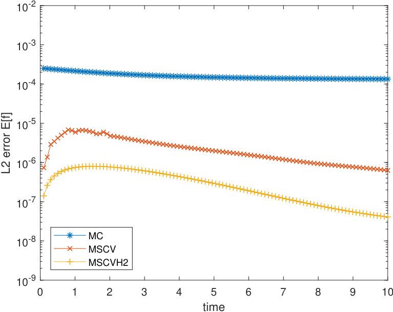 Figure 1
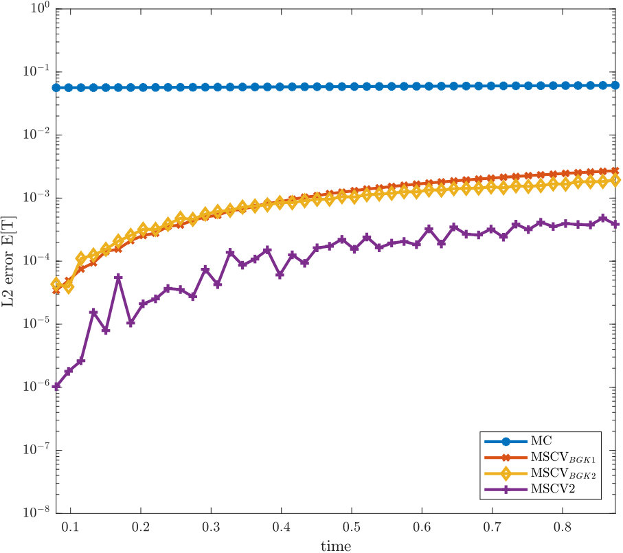 Figure 2
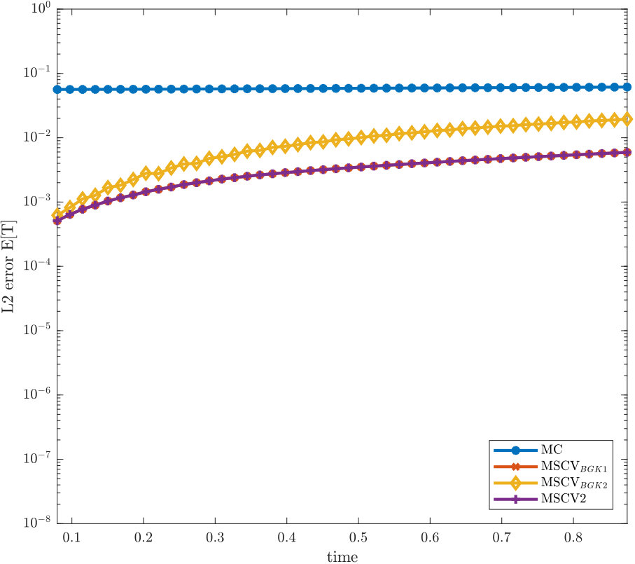 Figure 3
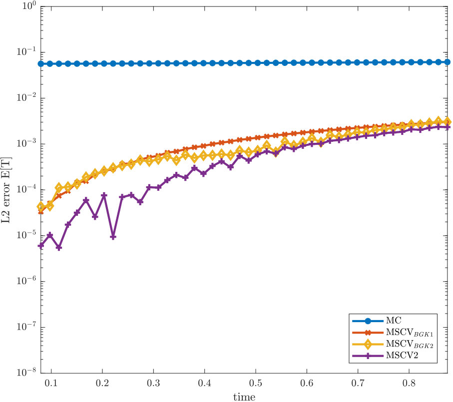 Figure 4
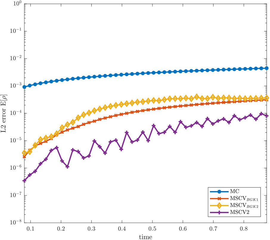 Figure 5
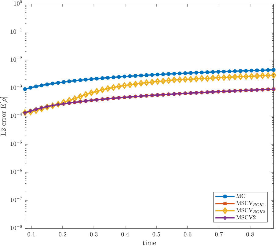 Figure 6
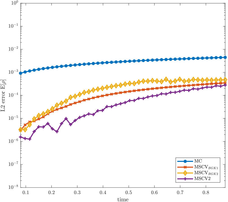 Figure 7
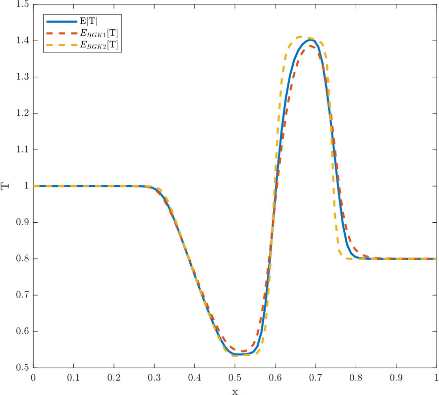 Figure 8
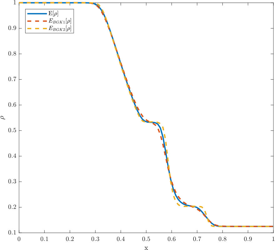 Figure 9
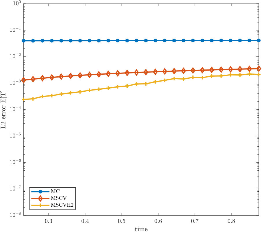 Figure 10
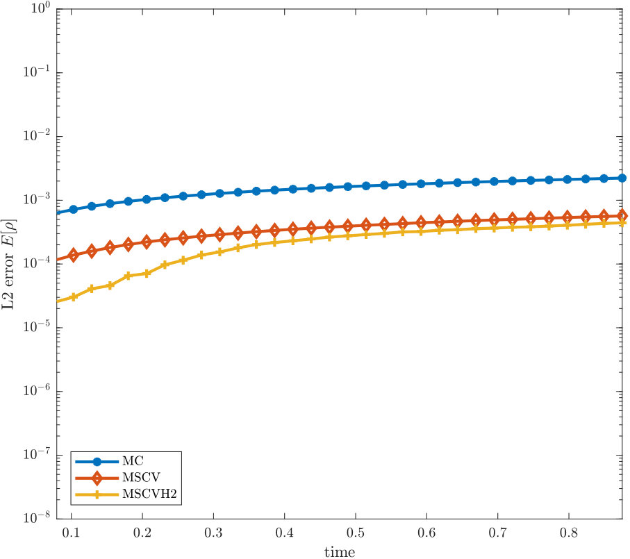 Figure 11
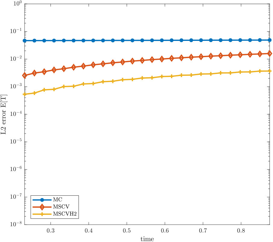 Figure 12
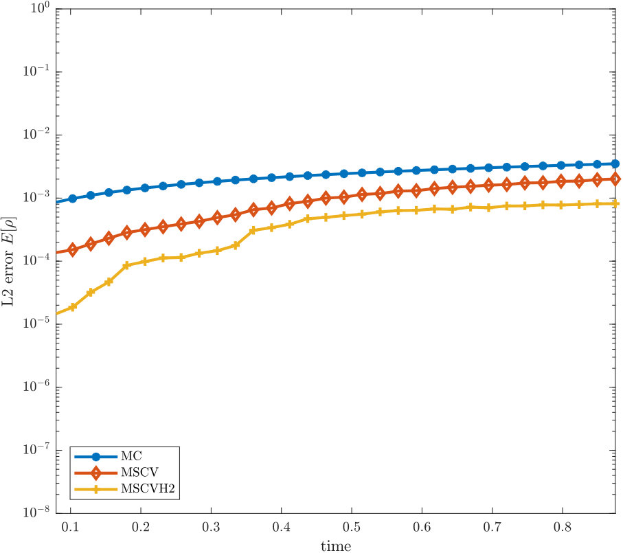 Figure 13
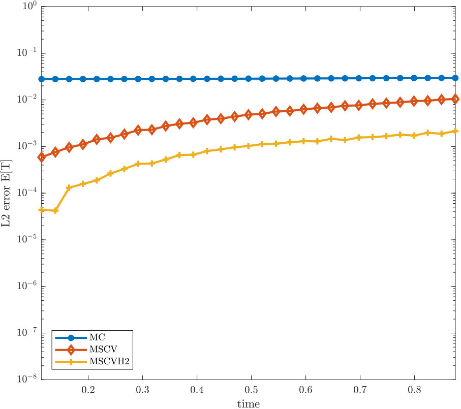 Figure 14
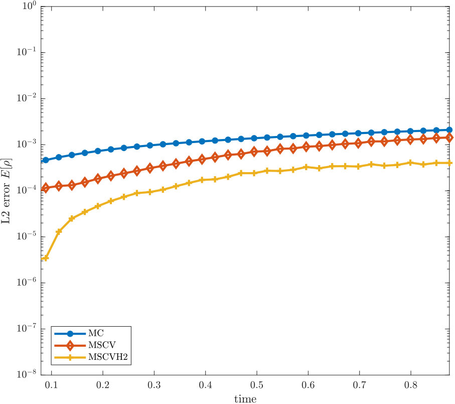 Figure 15
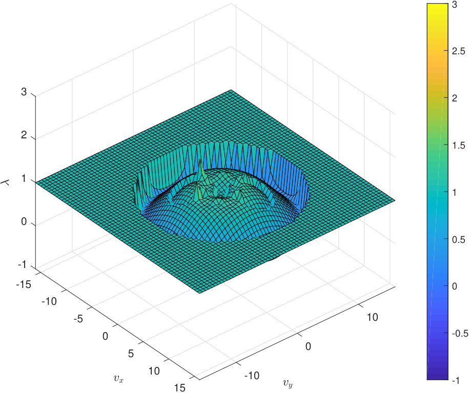 Figure 16
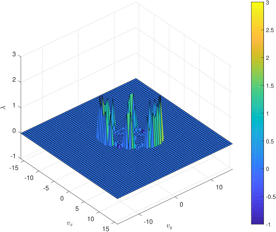 Figure 17
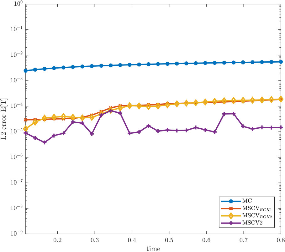 Figure 18
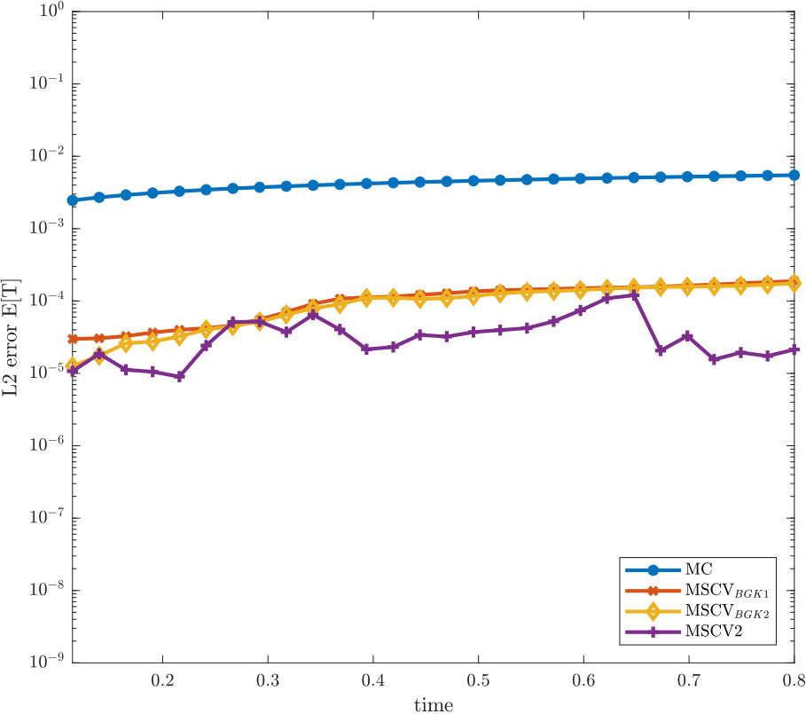 Figure 19
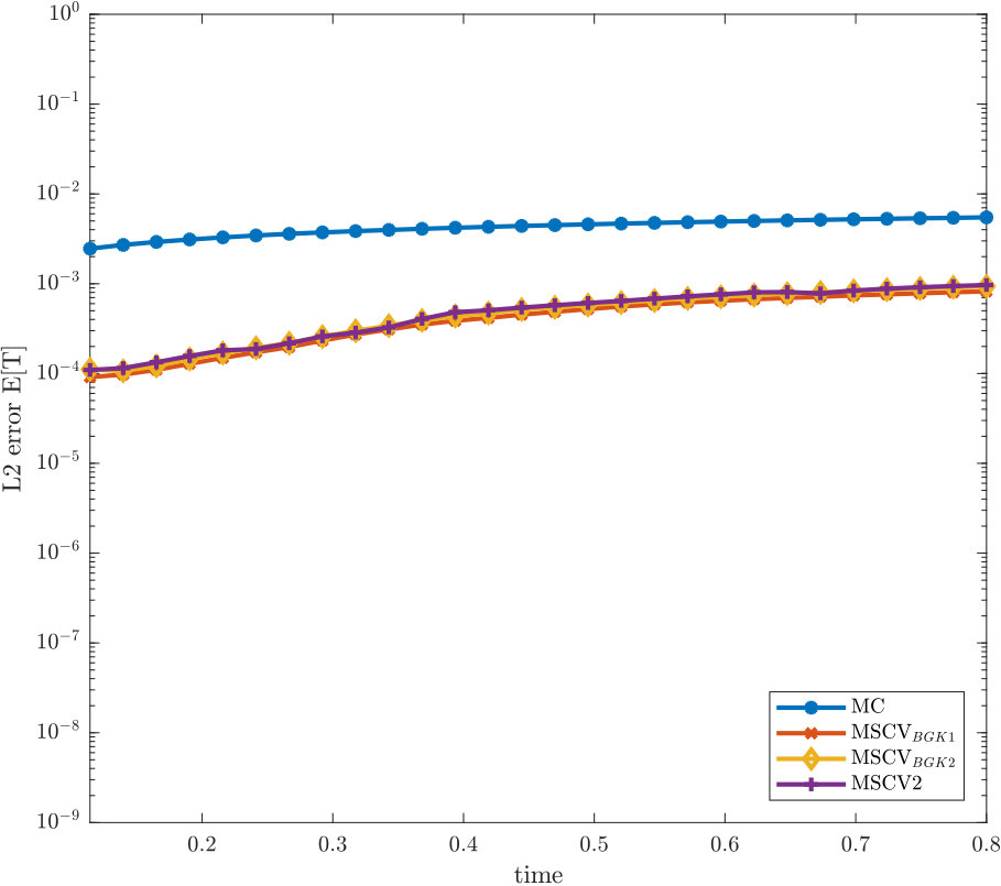 Figure 20
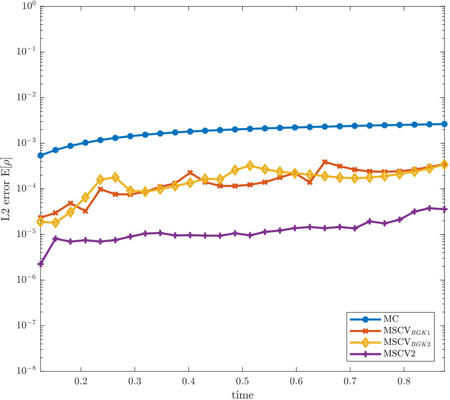 Figure 21
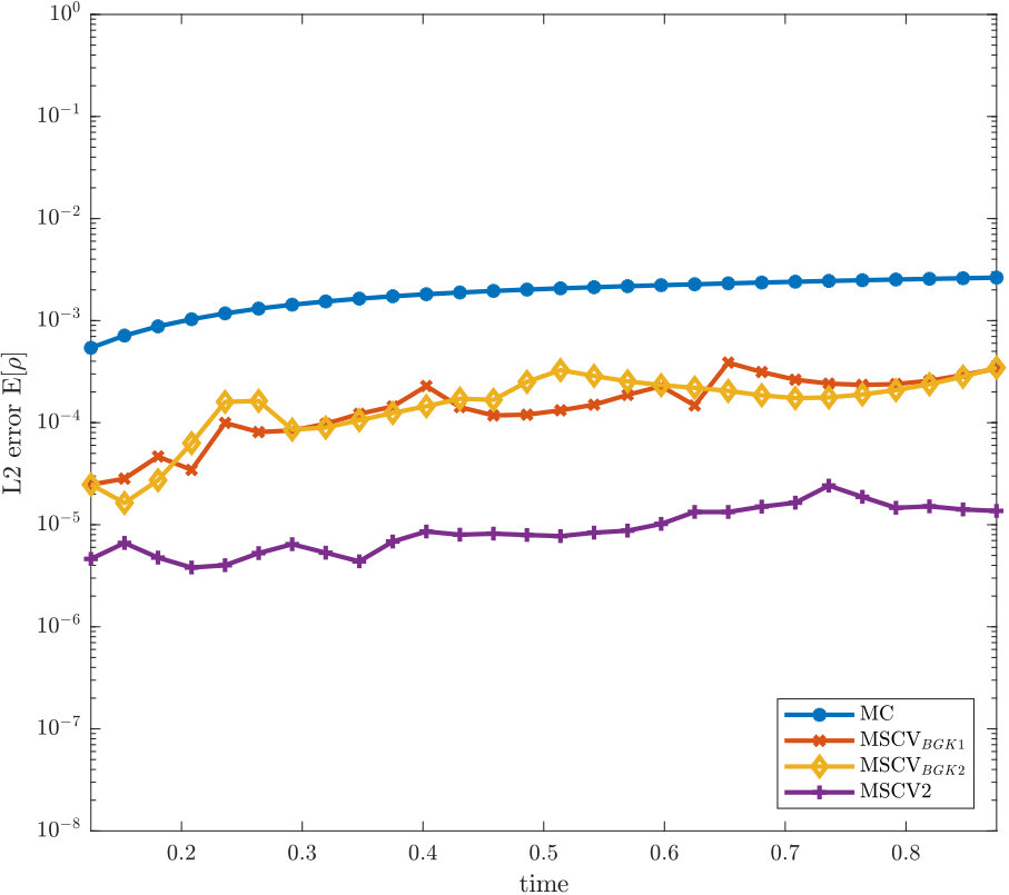 Figure 22
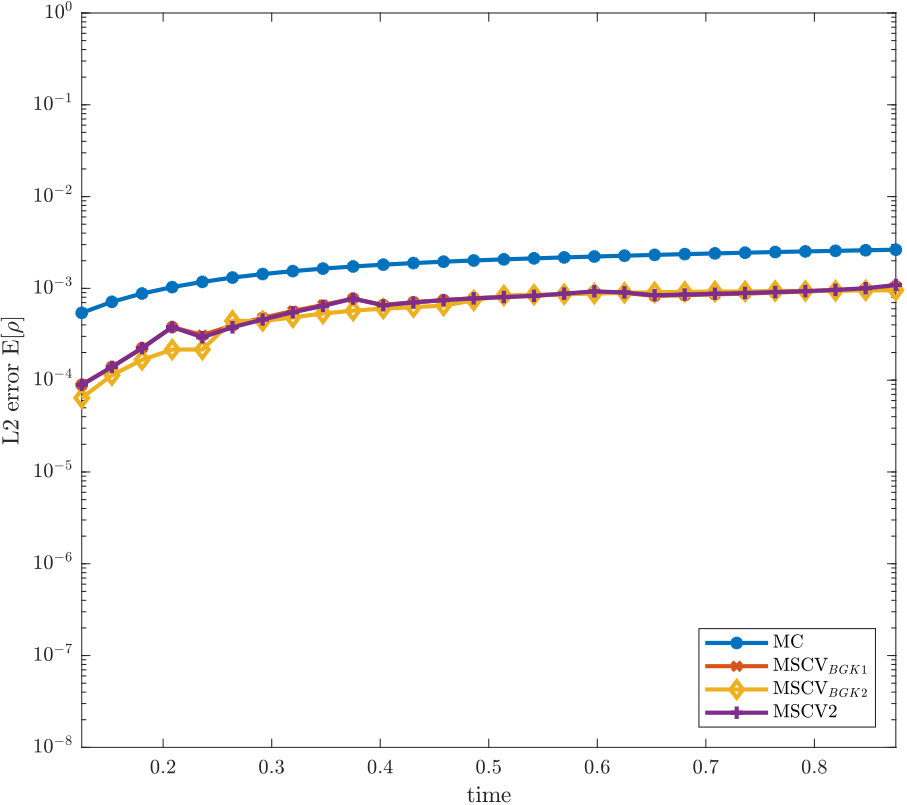 Figure 23
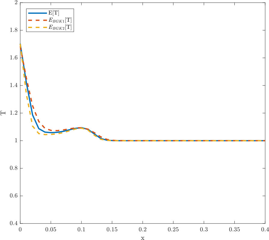 Figure 24
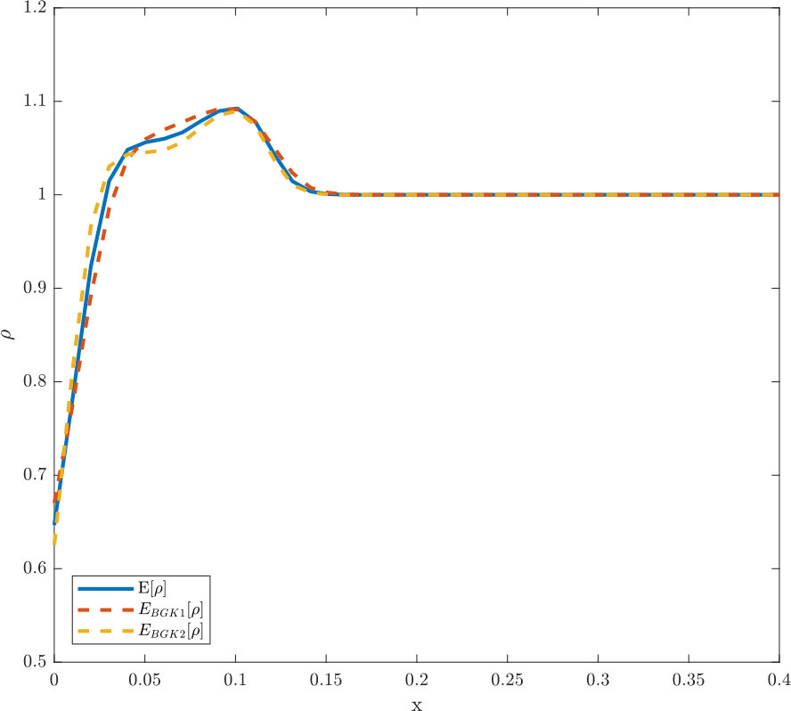 Figure 25
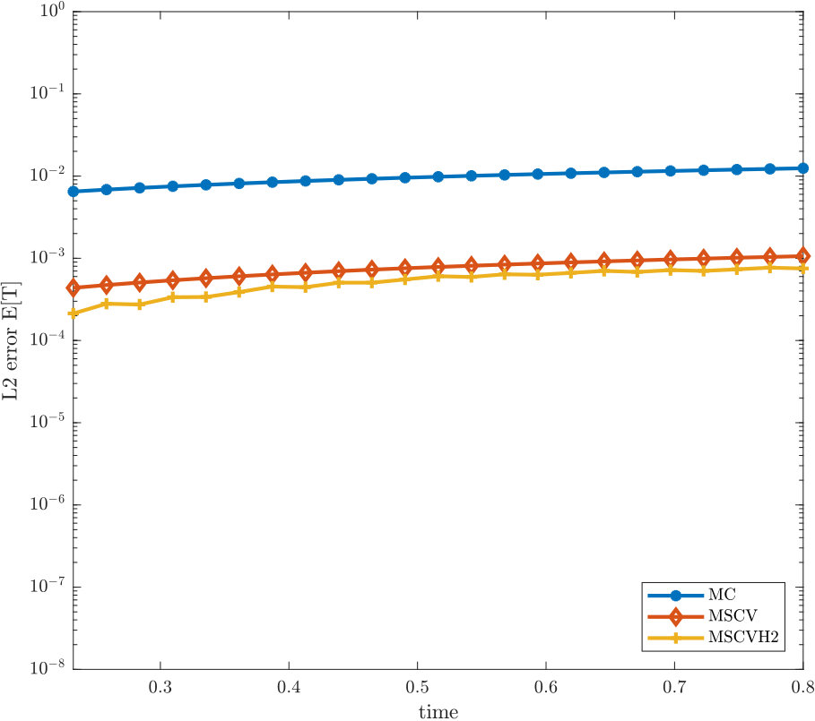 Figure 26
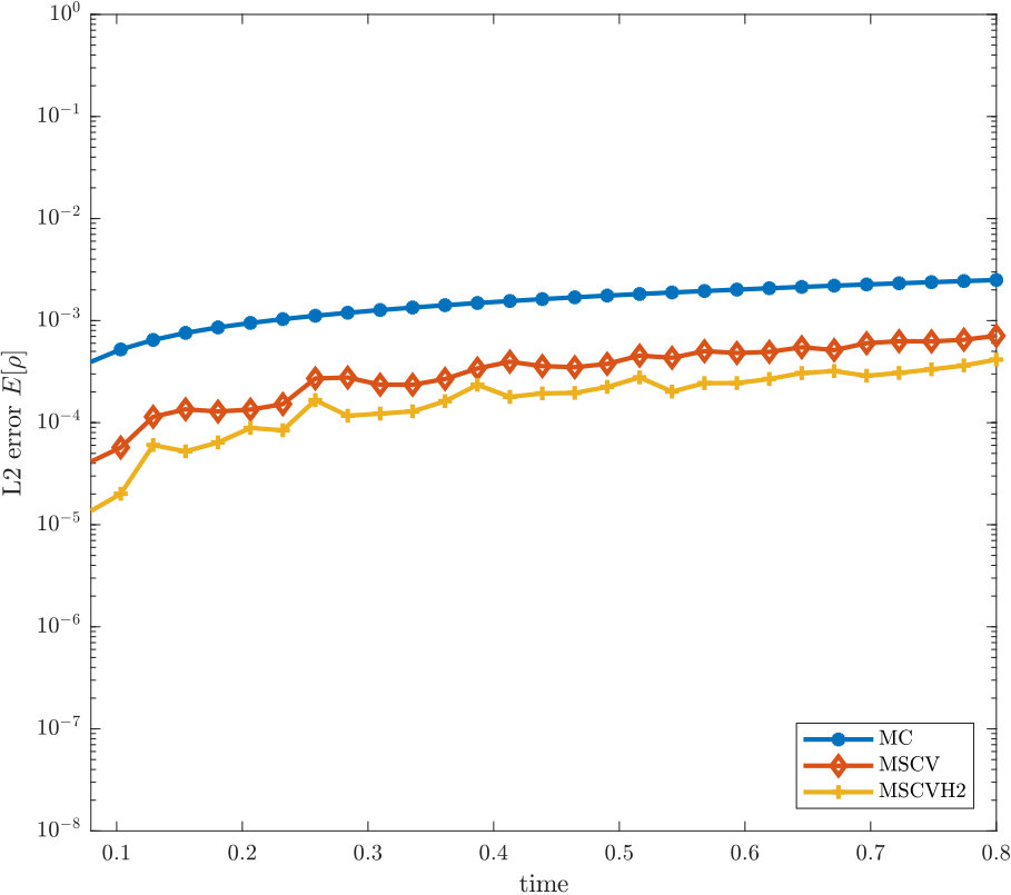 Figure 27
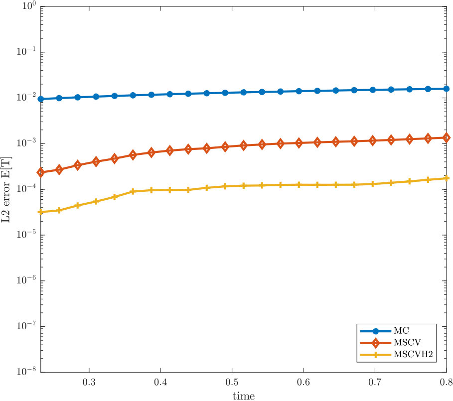 Figure 28
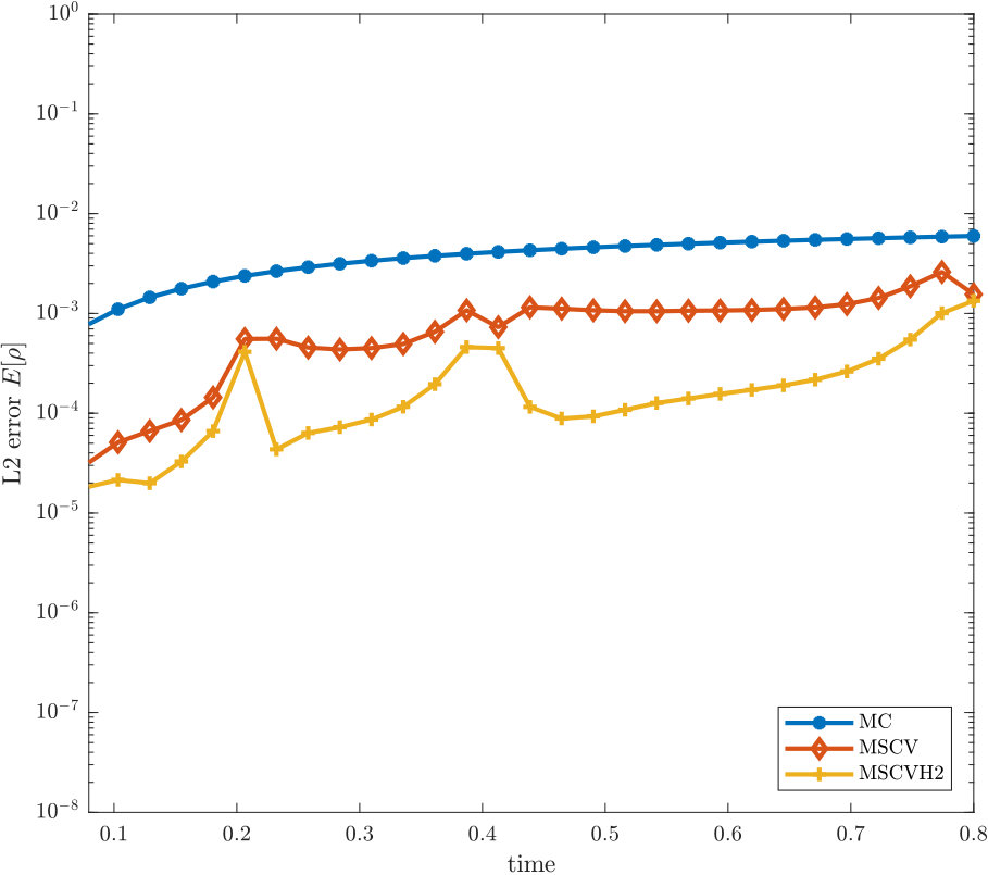 Figure 29
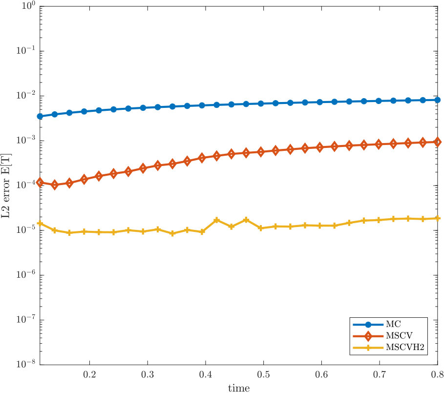 Figure 30
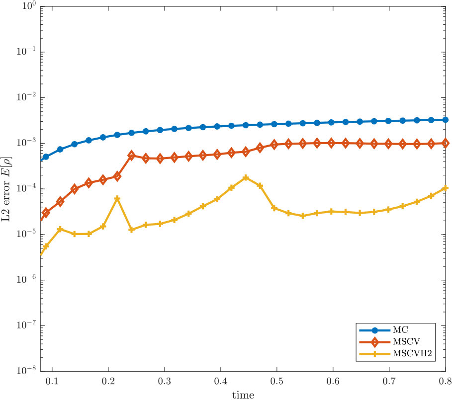 Figure 31
Peer Reviews
No public reviews on file for this paper yet. If you reviewed it on a platform where reviews are public (OpenReview, ICLR, NeurIPS, ICML), you can paste yours below so the community can read it here.
Videos
No videos yet. Explain this paper in a talk, walkthrough, or lecture? Add one.
Multi-scale variance reduction methods based on multiple control variates for kinetic equations with uncertainties111The research that led to the present article was partially supported by the INdAM-GNCS 2018 project Numerical methods for multi-scale control problems and applications.
Giacomo Dimarco222Department of Mathematics & Computer Science, University of Ferrara, Via Machiavelli 30, Ferrara, 44121, Italy ([email protected]). and Lorenzo Pareschi333Department of Mathematics & Computer Science, University of Ferrara, Via Machiavelli 30, Ferrara, 44121, Italy ([email protected]).
Abstract
The development of efficient numerical methods for kinetic equations with stochastic parameters is a challenge due to the high dimensionality of the problem. Recently we introduced a multiscale control variate strategy which is capable to accelerate considerably the slow convergence of standard Monte Carlo methods for uncertainty quantification. Here we generalize this class of methods to the case of multiple control variates. We show that the additional degrees of freedom can be used to improve further the variance reduction properties of multiscale control variate methods.
keywords:
Uncertainty quantification, kinetic equations, Monte Carlo methods, multiple control variates, multi-scale methods, multi-fidelity methods
AMS:
76P05, 65M75, 65C05
1 Introduction
Hyperbolic and kinetic equations with random inputs have attracted a lot of attention in the recent years [4, 15, 17, 22, 28, 27, 39]. Most of the literature on kinetic equations is based on the use of Stochastic-Galerkin methods based on on generalized Polynomial Chaos [1, 13, 38, 18, 15, 16, 31] and only recently these problems have been analyzed in the framework of statistical sampling methods based on Monte Carlo (MC) techniques [2, 10, 23, 7, 15, 9, 12].
When dealing with kinetic equations, MC sampling methods present several advantages since they afford simple integration of existing fast deterministic numerical solvers and parallelization techniques which are essential to reduce the computational complexity of many kinetic equations [8, 6, 5]. In addition MC methods are effective when the probability distribution of the random inputs is not known analytically or lacks of regularity when approaches based on stochastic orthogonal polynomials may be impossible to use or may produce poor results [20, 37].
Recently in [7] we introduced a control variate technique which takes advantage of the multi-scale nature of the kinetic equation which is capable to strongly accelerate the slow convergence of MC methods. In this manuscript we generalize this class of multi-scale control variate methods (MSCV) to the case of multiple-control variates. In particular we will show how the use of additional control variates functions permit to further reduce the statistical variance of the methods. We refer to [24, 25] for related approaches in the general framework of multifidelity models.
From a mathematical viewpoint, we consider kinetic equations of the general form [3, 7]
[TABLE]
where , , , , , and , , is a random variable. In (1.1) the parameter is the Knudsen number and the particular structure of the interaction term depends on the kinetic model considered.
The most famous example is represented by the nonlinear Boltzmann equation of rarefied gas dynamics
[TABLE]
where and
[TABLE]
Before going into the details of the presentation we introduce some notations and assumptions that will be used in the sequel. If is distributed as we denote the expected value by
[TABLE]
and we introduce the following -norm with polynomial weight [26, 30]
[TABLE]
Next, for a random variable taking values in , we define
[TABLE]
The above norm, if , differs from
[TABLE]
used for example in [20]. Note that by Jensen inequality [29] we have
[TABLE]
To avoid unnecessary difficulties in the sequel we consider norm (1.6) for . The same results hold true for (the two norms coincides) whereas their extension to norm (1.7) for typically requires to be compactly supported. We refer to [20, 7] and [15, Chapter 7] for further details.
Finally, we assume that the deterministic solver for (1.1), if the initial data is sufficiently regular, satisfies the estimate (see [30, 8, 32, 7, 21])
[TABLE]
with a positive constant which depends on time and on the initial data, and the computed approximation of the deterministic solution at time on the mesh and . Here the positive integers and characterize the accuracy of the discretizations in the phase-space and for simplicity, we ignored the errors due to the time discretization and to the truncation of the velocity domain in the deterministic solver [8]. We emphasize that the estimates here presented are purposely of a general nature to illustrate the characteristics of the method, the application to specific kinetic models can clearly lead to more targeted estimates but it is outside the objectives of the present work.
The remaining sections can be summarized as follows. In the next Section we survey the MSCV methods introduced in [7]. Then, in Section 3 we extend these multi-scale approaches to the case of multiple control variates. First we introduce a standard multiple control variate approach and then consider the construction of recursive multiple control variate methods based on a hierarchical structure. A particular attention is devoted to the case of two control variates. Section 4 is devoted to present several numerical examples confirming the capability of the multiple control variate approach to provide a strong variance reduction with respect to standard Monte Carlo and to further improve the methods based on a single control variate. Some conclusions are reported at the end of the manuscript.
2 Multi-scale control variate methods
In this section we survey the MSCV approach recently introduced in [7]. The main idea of the method is to reduce the variance of standard Monte Carlo estimators using as control variate the solution of a simpler kinetic model, which can be evaluated at a fraction of the cost of the full model, with the same fluid limit behavior. We illustrate the method when applied to the solution of a kinetic equation of the type (1.1) with deterministic interaction operator and random initial data .
2.1 Variance reduction strategies
Let us first consider the space homogeneous problem
[TABLE]
where and with random initial data . In (2.1), without loss of generality, we have fixed since in the space homogeneous case the Knudsen number scales with time. Under suitable assumptions, one can show that exponentially decays to the unique steady state such that which satisfies
[TABLE]
for some moments, for example in the classical settings of conservation of mass, momentum and energy (see [36, 35, 34, 33]). We emphasize that, for many space homogeneous kinetic models, the equilibrium state can be computed directly from the initial data thanks to the conservation properties (2.2).
We recall that, given independent identically distributed (i.i.d.) samples , , of the solution to (2.1), the standard Monte Carlo estimator reads
[TABLE]
The above estimator satisfies [20, 7]
[TABLE]
where and is the variance.
A simple variance reduction strategy is obtained by splitting the expected value of the solution as
[TABLE]
and exploiting the fact that can be evaluated with arbitrary accuracy at a negligible cost (for example using a very fine grid of samples) since it does not depend on the solution computed at each time step.
Now, if we use (2.5) and estimate
[TABLE]
we obtain an error of the type
[TABLE]
Since the non equilibrium part goes to zero in time exponentially fast, then also its variance goes to zero, which means that for long times estimate (2.6) becomes exact and depends only on the accuracy of the evaluation of .
The above argument can be generalized by considering a time dependent approximation of the solution , whose evaluation is significantly cheaper than computing , such that for some moments and that as .
For example, one can consider the space homogeneous Boltzmann equation (2.1) where is given by (1.2) and assume to be the exact solution of the space homogeneous BGK approximation
[TABLE]
with independent from and for the same initial data . Thanks to the time invariance of the equilibrium state we have and we can write the exact solution to (2.7) as
[TABLE]
We can assume that the expected value of the control variate is computed with arbitrary accuracy at a negligible cost since it is a convex combination of the initial data and the equilibrium part. We denote this value by
[TABLE]
where and or accurate approximations of the same quantities.
If we now use the estimator
[TABLE]
we have an error like
[TABLE]
where even in this case, as .
2.1.1 Control variate estimators
The simple variance reduction argument presented in the previous section can be used to formalize the following control variate estimator [7]
[TABLE]
The control variate estimator (2.11) is unbiased and consistent for any choice of . In particular, for we recover the standard MC estimator , whereas for we have the estimator corresponding to (2.10).
If we now consider the random variable
[TABLE]
we have , and we can quantify its variance as
[TABLE]
We have the following [7]
Theorem 1**.**
The quantity
[TABLE]
minimizes the variance of at the point and gives
[TABLE]
where is the correlation coefficient between and . In addition, we have
[TABLE]
Using such an approach, in combination with a deterministic solver satisfying (1.9), one obtains the following error estimate [7, 20]
[TABLE]
where , and depends on the final time and on the initial data. Here we ignored the statistical errors due to the approximation of the control variate expectation and to the estimate of . Note that, since as the statistical error will vanish for large times.
Remark 2.1**.**
In practice, appearing in is not known and has to be estimated. Starting from the samples we have the following unbiased estimators
[TABLE]
which allow to estimate
[TABLE]
It can be verified easily that as .
2.2 Multiscale control variate estimators
Let us now consider the full space non homogeneous problem (1.1). Again the idea is to compute the control variate function with a simplified model which can be evaluated at a fraction of the computational cost of the full model. However, in the space non homogeneous case the expectation of the control variate typically depends on time and must be estimated along the simulation.
Assuming the classical setting of the Boltzmann equation (1.1)-(1.2), where the collision term characterizes conservation of mass, momentum and energy, integration of (1.1) with respect to the collision invariants gives the moments equations
[TABLE]
where , with density, mean velocity and temperature defined as
[TABLE]
and
[TABLE]
Now, generalizing the space homogeneous method based on the local equilibrium as control variate we can consider the Euler closure as control variate, namely to assume in (2.20). If we denote by the solution of the fluid model
[TABLE]
for the same initial data, the corresponding equilibrium state can be used as control variate.
Similarly to the homogeneous case, the generalization to an improved control variate based on a suitable approximation of the kinetic solution can be done with the aid of a more accurate fluid approximation, like the compressible Navier-Stokes system, or a simplified kinetic model. In the latter case, we can solve a BGK model
[TABLE]
for the same initial data and use its solution as control variate.
More precisely, given i.i.d. samples of the solution and of the control variate we define the estimator
[TABLE]
where is an accurate approximation of .
The fundamental difference is that now the variance of
[TABLE]
will not vanish asymptotically in time since , unless the kinetic equation is close to the fluid regime, namely for small values of the Knudsen number. Thus, the first part of Theorem 2.15 is still valid, however the optimal value
[TABLE]
and the variance
[TABLE]
now satisfy
[TABLE]
In fact, since as from (1.1) we formally have which implies and , from (2.25) and (2.26) we obtain (2.27).
Even if simulating the control variate system is much cheaper than the full model, since its computational cost is no more negligible we cannot ignore it. Thus, we assume that the control variate model is computed over a fine grid of samples and use the approximation
[TABLE]
in the estimator (2.24) which we will denote by .
This, however, has an impact on the optimal value of in estimator (2.24). In fact, using the independence of and and the fact that by the central limit theorem [19, 12] we have , , minimizing the variance now leads to the optimal value
[TABLE]
with given by (2.25). This correction may be relevant in the cases when and do not differ too much. In our setting, however, so that and we can assume .
Using the optimal value (2.25) and an underlaying deterministic solver which satisfies (1.9), we obtain the error estimate [7, 20]
[TABLE]
where , , the constant depends on the final time and on the initial data. Now, as , therefore in the fluid limit we recover the statistical error of the fine scale control variate model.
Remark 2.2**.**
For space non homogeneous simulations, since we typically are interested in the evolution of the moments, one can compute the optimal value of with respect to a given moment as
[TABLE]
where is defined by (2.2), so that . This approach leads to a value of which depends on the moment evaluated and, since is independent of the velocity, strongly reduces the storage requirements. Note that, using (2.30) all estimates in this section for translates easily into estimates for .
3 Multiple multi-scale control variates
The approach described in Section 2 is fully general and accordingly to the particular kinetic model studied one can select a suitable approximated solution as control variate which acts at a given scale. In this section we extend the methodology to the use of several approximated solutions as control variates with the aim to further improve the variance reduction properties of MSCV methods.
3.1 Multiple control variates
To keep notations simple we describe the method in the case of the space homogeneous equation (2.1), the extension to the space non homogeneous case follows analogously to Section 2.2 and is discussed at the end of the Section.
Let us consider approximations of solution to (2.1) whose properties will be discussed later. We can define the random variable
[TABLE]
Clearly (3.1) is such that and has variance
[TABLE]
In vector form, if we introduce notations
[TABLE]
we have
[TABLE]
where , is the symmetric covariance matrix.
Theorem 2**.**
Assuming the covariance matrix is not singular, the vector
[TABLE]
minimizes the variance of at the point and gives
[TABLE]
Proof.
To compute the minimizing values , the first order optimality conditions are found by equating to zero the partial derivatives with respect to
[TABLE]
This corresponds to solve the following linear system
[TABLE]
or in vector form
[TABLE]
Therefore, assuming the covariance matrix is not singular, we obtain the solution (3.3). It is easily shown, via the second order optimality conditions that is indeed the variance-minimizing choice of . By direct substitution in (3.2) we obtain (3.4). ∎
The control variate estimator based on (3.1) takes the form
[TABLE]
where is an accurate approximation of , and we assumed to have i.i.d. samples from the solution and the control variate functions for . To estimate the value of the vector we can use directly the Monte Carlo samples as in the scalar case. The resulting MSCV algorithm is summarized as follows:
Algorithm 3.1** (Multiple MSCV - homogeneous case).**
Sampling*: Sample i.i.d. initial data from the random initial data and approximate these over the grid . Denote these samples by , .* 2. 2.
Solving*:*
- (a)
For each control variate and for each realization of the random input data , , the resulting control variate model is solved numerically by a deterministic solver with mesh width . We denote the resulting ensemble of deterministic solutions for at time by
[TABLE] 2. (b)
For each realization , the underlying kinetic equation (2.1) is solved numerically by the corresponding deterministic solver with mesh width . We denote the solution at time by , . 3. 3.
Estimating*:*
- (a)
Estimate the optimal vector of values solving
[TABLE]
where and . 2. (b)
Compute the expectation of the random solution with the control variate estimator
[TABLE]
Let us remark that, if we introduce the vector , such that , , , then equation (3.1) reads
[TABLE]
and thus, the variance of is reduced to zero if is in the span of the set of functions .
Using Gram–Schmidt orthogonalization, we may assume that the components of the control variate vector are orthogonal in the inner product
[TABLE]
In fact, we have
[TABLE]
We can construct the vector , with orthogonal components, for , as follows [11]
[TABLE]
and define , such that , .
Then we may try to minimize the variance of the random variable
[TABLE]
which now using the orthogonality property reads
[TABLE]
Denoting with , the diagonal matrix with elements and with the vector with components we get
[TABLE]
By the same arguments as in Theorem 3.4, if the matrix is not singular, we have that the vector minimizes the above variance. Thus we have proved the following result.
Theorem 3**.**
If the control variate vector in (3.13) has orthogonal components, for , then if the vector with components
[TABLE]
minimizes the variance of at the point and gives
[TABLE]
where is the correlation coefficient between and .
Estimating the orthogonal set of control variates using samples by
[TABLE]
where or its accurate approximation, in combination with a deterministic solver satisfying (1.9), one obtains the following result [7, 20].
Proposition 4**.**
Consider a deterministic scheme which satisfies (1.9) in the velocity space for the solution of the homogeneous kinetic equation (2.1) with deterministic interaction operator and random initial data . Assume that the initial data is sufficiently regular.
Then, the MSCV estimate defined in (3.17) with the optimal values given by (3.15) satisfies the error bound
[TABLE]
where , and depends on the final time and on the initial data.
Proof.
The bound follows from
[TABLE]
where the Monte Carlo bound in the first term now make use of (3.16) and the second term is bounded by the discretization error of the deterministic scheme. ∎
Here we ignored the statistical errors due to the approximation of the control variates expectations and to the estimate of the vector .
3.1.1 Two control variates
To exemplify the approach, it is interesting to consider the case , where , the initial data, and , the stationary state. In this case we know that is in the span of the control variates at and as .
A straightforward computation shows that the optimal values and are given by
[TABLE]
where .
Using samples for both control variates the optimal estimator reads
[TABLE]
Now, at since we clearly have and so that the estimator (3.20) is exact
[TABLE]
Moreover, by the same arguments as in Theorem 2.15, for large times since from (LABEL:eq:l12) we get
[TABLE]
and thus, the variance of the estimator vanishes asymptotically in time
[TABLE]
We emphasize that this last example can be seen as a generalization of the scalar case based on the BGK model. In fact, the estimator (2.11) based on (2.8)-(2.9) can be written in the form (3.20) as
[TABLE]
where
[TABLE]
Therefore, the scalar control variate based on the BGK model can be understood as a suboptimal solution to the our minimization problem for the control variates and . In particular, if the solution has the form (2.8), namely the full model is the BGK model, then it is in the span generated by and and we obtain and .
3.2 Hierarchical multiple control variates
The multiple control variate approach just described presents some limitations. First the linear system (3.9) may be difficult to solve due to ill conditioning of the covariance matrix and additionally the estimation of the coefficients in the matrix requires the use of a control variate independent number of samples. This last aspect can represent a serious limitation in space non homogeneous situations in which the control variates may be originated from models that operate at the various spatio-temporal scales of the problem with different levels of complexity.
To overcome such drawbacks here we formulate a recursive construction of the multiple control variate estimator (3.8). To this aim, let us assume that the control variates represent kinetic models with an increasing level of fidelity. Under this assumption the control variate represents the less accurate model whereas the control variate is the closer model to the full model .
To start with, we estimate with samples using as control variate
[TABLE]
Next, to estimate of we use samples and consider as control variate
[TABLE]
Similarly, in a recursive way we can construct estimators for the remaining expectations of the control variates using respectively samples until
[TABLE]
and we stop with the final estimate
[TABLE]
with .
By combining the estimators of each stage together we obtain the recursive MSCV estimator
[TABLE]
Now if we compute the optimal values independently for each recursive stage by ignoring the errors due to the approximations of the various expectations, if , we obtain
[TABLE]
where we used the notation . We refer to this set of values, which avoids the solution of the resulting linear system, as quasi-optimal. Note that, since the control variates and are known on the same set of samples the values can be estimated using (2.17)-(2.18).
The estimator (LABEL:eq:lambdar) can be recast in the form
[TABLE]
where we defined
[TABLE]
Since by the central limit theorem [19, 12] we have , using the independence of the estimators , , the total variance of the estimator (LABEL:eq:mscvgr) is
[TABLE]
Now, the first order optimality conditions
[TABLE]
leads to the tridiagonal system for
[TABLE]
or equivalently
[TABLE]
where we assumed and . The resulting system can be solved efficiently by the usual Thomas algorithm for tridiagonal systems provided , .
System (3.26) can be rewritten as
[TABLE]
which, reverting to the original control variate variables becomes
[TABLE]
Thus, the quasi-optimal values (3.22) solves the above system up to .
Theorem 5**.**
The vector solution of the tridiagonal system (3.26) minimizes the variance of the estimator (LABEL:eq:mscvgr). In particular the vector of quasi-optimal solutions given by (3.22) is such that
[TABLE]
where .
Proof.
We can rewrite (3.26) in the form where with
[TABLE]
, , and , . By construction the vector , such that , minimizes the variance of (LABEL:eq:mscvgr).
Let us define the vector of elements , where are given by (3.22). We have so that
[TABLE]
therefore if , we can write
[TABLE]
Now, since is upper triangular and diagonal we have (3.27). ∎
We can summarize the details of the method, when applied to the space homogeneous problem (2.1) in combination with a deterministic solver, in the following algorithm.
Algorithm 3.2** (Recursive multiple MSCV - homogeneous case).**
Sampling*: For each control variate , we draw a number of i.i.d. samples from the random initial data and approximate these over the mesh . Denote these control variate dependent number of samples for by*
[TABLE]
and set . 2. 2.
Solving*:*
- (a)
For each control variate and for each realization of the random input data , , the resulting control variate model is solved numerically by a deterministic solver with mesh widths . We denote the resulting ensemble of deterministic solutions for at time by
[TABLE] 2. (b)
For each realization , the underlying kinetic equation (1.1) is solved numerically by the corresponding deterministic solver with mesh widths . We denote the solution at time by , . 3. 3.
Estimating*:*
- (a)
Estimate the optimal vector of values as
[TABLE]
where we used the notation , . 2. (b)
Compute the expectation of the random solution with the control variate estimator
[TABLE]
where
[TABLE]
Regarding the error bound that we obtain using (LABEL:eq:mscvgr) with the values given by (3.22) le us observe that if, at each stage, we denote
[TABLE]
then by the error bound (2.29) we have
[TABLE]
where is a suitable constant and we defined
[TABLE]
Using the recursive estimator, in combination with a deterministic solver satisfying (1.9), we can write
[TABLE]
The second term is bounded as usual by the discretization error of the scheme, whereas, ignoring the statistical errors in estimating the quasi-optimal vector of values , the first term can be estimated recursively as
[TABLE]
where we defined
[TABLE]
Thus we have proved the following result
Proposition 6**.**
Consider a deterministic scheme which satisfies (1.9) in the velocity space for the solution of the homogeneous kinetic equation (2.1) with deterministic interaction operator and random initial data . Assume that the initial data is sufficiently regular.
Then, the recursive MSCV estimate defined in (LABEL:eq:lambdar) with satisfies the error bound
[TABLE]
where are given by (3.32), and depends on the final time and on the initial data.
Finally, concerning the relations between the recursive MSCV estimator (LABEL:eq:mscvgr) and the Multi-level Monte Carlo (MLMC) approach [20, 7], we made the following remarks.
Remark 3.1**.**
- •
We can emphasize the analogies with MLMC by using as control variates a hierarchy of discretizations of the kinetic equation with random inputs. In the case of a cartesian grid this aims at constructing a velocity discretization with corresponding mesh width that satisfy , where is the mesh width for the coarsest resolution. To avoid unessential difficulties, we denote by , , the continuous representation, for example by polynomial interpolation, of the corresponding numerical solution at time obtained with the underlaying deterministic method using mesh width .
Under these assumptions, fixing , in (LABEL:eq:mscvgr), we get the classical MLMC estimator **[10]**
[TABLE]
where we used the notation . Note that, as a side result of our derivation, using the quasi-optimal values (3.22) in (LABEL:eq:mscvgr) (or the optimal values solution to (3.26)) with the hierarchical grid constructed above we obtain a quasi-optimal (optimal) version of MLMC.
- •
Similarly to MLMC methods, in the recursive MSCV estimator (LABEL:eq:mscvgr) the largest number of samples is required on the less accurate model , where the samples are cheaper, whereas only a small number of samples are needed on the full model. The two key differences between the recursive MSCV estimator (LABEL:eq:mscvgr) and the MLMC approach (3.34) consist in the choice of low fidelity models as control variates instead of a hierarchy of discretizations and in using the quasi-optimal values (3.22) (or the optimal values solution to (3.26)) instead of fixing , .
3.3 Multiple multi-scale control variates estimators
For non homogeneous problems, as in the scalar case summarized in Section 2.2, the main difference is that we cannot assume to know the expectation of the control variate or that it can be computed accurately at a negligible computational cost. Each control variate, in fact, acts at a certain scale and requires the numerical solution of a suitable time dependent model in the phase space.
Now, the MSCV estimator (3.8), based on the multiple control variates , , for the solution to problem (1.1), reads
[TABLE]
where samples have been used to estimate the expectations of the control variates .
As in the scalar case, minimization of the variance of (3.35), leads to the optimal values
[TABLE]
with given by (3.3). In the sequel we assume so that .
The extension of algorithms 3.1 to the non homogeneous case is reported below.
Algorithm 3.3** (Multiple MSCV - non homogeneous case).**
Sampling*:*
- (a)
Sample i.i.d. initial data , from the random initial data and approximate these over the grid characterized by and . 2. (b)
Sample i.i.d. initial data , from the random initial data and approximate these over the grid characterized by and . 2. 2.
Solving*:*
- (a)
For each control variate and for each realization , , the resulting control variate model is solved numerically by a deterministic solver with mesh widths . We denote the resulting deterministic solutions for at time by , and estimate their expectations by
[TABLE] 2. (b)
For each realization , the underlying kinetic equation (1.1) is solved numerically by the corresponding deterministic solver with mesh widths . We denote the solution at time by , . 3. 3.
Estimating*:*
- (a)
Estimate the optimal vector of values solving
[TABLE]
where and . 2. (b)
Compute the expectation of the random solution with the control variate estimator
[TABLE]
In the space non homogeneous case, similarly to the case where the control variates expectations are known, we can apply the Gram–Schmidt orthogonalization procedure (3.12) and use the estimator
[TABLE]
with the optimal vector of values defined by (3.15). For the estimator (3.39) we have the following generalization of the error estimate (3.18).
Proposition 7**.**
Consider a deterministic scheme which satisfies (1.9) for the solution of the kinetic equation of the form (1.1) with deterministic interaction operator and random initial data . Assume that the initial data is sufficiently regular.
Then, the MSCV estimate defined in (3.39) with the optimal values given by (3.15) satisfies the error bound
[TABLE]
with , , and depends on the final time and on the initial data.
Proof.
We have
[TABLE]
The first term can be bounded similarly to (3.18) to get
[TABLE]
Using the fact that, ignoring the statistical error in estimating , from (3.17) and (3.39) we have
[TABLE]
From (3.15) the second term can be bounded by
[TABLE]
∎
Similarly, the recursive MSCV estimator (LABEL:eq:mscvgr), based on a hierarchy of multiple control variates , , with increasing level of fidelity for the solution to problem (1.1), is
[TABLE]
with and where now the optimal values of are obtained from the quasi-optimal solution (3.22) using (3.24) or by the correction introduced by the solution of the tridiagonal system (3.26) if relevant.
In this case, the extension of algorithms 3.2 and estimate (3.33) to the non homogeneous case follows straightforwardly simply replacing and with and , and is omitted for brevity.
Finally, due to its importance in practical applications, we describe the details of the hierarchical method in the case .
3.3.1 Two multi-scale hierarchical control variates
Let us focus on the case of a recursive multiscale estimator with two control variates . To this aim we consider as the equilibrium state associated to the system of Euler equations
[TABLE]
with , and corresponding to the limit case in (1.1). As a second control variate we consider as the solution of the BGK model
[TABLE]
Both models are solved for the same initial data . Now, the Euler equations are used as control variate to improve the computation of the expectation in the BGK model, that in turn is used as control variate to improve the computation of the expectation in the full Boltzmann model.
The recursive estimator now reads
[TABLE]
where . If we define and their optimal values are computed as solutions of system (3.26) for
[TABLE]
with , which gives
[TABLE]
The quasi-optimal values are obtained assuming and are characterized by
[TABLE]
In the fluid limit we have so that
[TABLE]
then
[TABLE]
On the contrary, the quasi-optimal values are such that
[TABLE]
and therefore
[TABLE]
which corresponds to the equilibrium solution over the finest grid of samples.
4 Numerical examples
In this Section, we discuss several numerical examples with the aim of illustrating the characteristics of the multiple control variate strategies described in the previous Sections. We focus on the two control variates approach 3.1.1 and on the multi-scale hierarchical multiple control variates one in the case where the hierarchy consists of two models with an increasing level of fidelity as described in Section 3.3.1. We use shorthands MC, MSCV, MSCV2 and MSCVH2 to denote, respectively, the standard Monte Carlo, the single multi-scale control variate, the multiple multi-scale control variates and the hierarchical multiple multi-scale control variates.
The first test problem consists of a space homogeneous case with uncertain initial data, the second test problem is a Riemann problem with uncertainties in the initial state while the third test problem has randomness in the boundary condition. These tests are analogous to those considered in [7] using a single control variate and our precise aim is to show that with a multiple control variates approach it is possible to achieve better results in terms of the ratio between computational cost and accuracy. In all our numerical tests the velocity space is two dimensional , the velocity domain is truncated to and the collision integral is solved by the fast spectral method [21, 8]. In the sequel, all the statistical errors have to be intended in the sense of the average where values have been used to compute the mean.
4.1 Space homogeneous Boltzmann equation
We consider the space homogeneous Boltzmann equation (2.1). We compare the case of the single control variate based on the BGK model 2.1.1 with the case of the two control variates approach of Section 3.1.1. The number of samples used to compute the expected solution for the Boltzmann equation is . Note that, since the control variates do not contribute to the overall computational cost their expected values are computed with high accuracy using orthogonal polynomials.
4.1.1 Test 1. Uncertain initial data
The initial condition is a two bumps problem with uncertainty
[TABLE]
with , , and uniform in . The velocity space is discretized with points. We choose . The time integration has been performed with a -th order Runge-Kutta method using and a final time .
In Figure 1, we report the error with respect to the random variable in the computation of the expected value for the distribution function for the various methods. Clearly, all MSCV methods provide a gain in accuracy of several orders of magnitudes with respect to standard Monte Carlo. In particular, we observe that MSCV2 method based on two control variates permits to gain one order of accuracy with respect to the standard MSCV approach.
In Figure 2 we report the shape of the optimization coefficients and at the final time. It is possible to observe that is approaching zero and is approaching one, except in the regions where the solution still differs from its equilibrium value.
4.2 Space non homogeneous Boltzmann equation
Next, we consider the space non homogeneous Boltzmann equation (1.1). Concerning the space-time discretization, we make use of a fifth order WENO method [14] for the spatial discretization and a second order explicit Runge-Kutta method for the time discretization. The time step is the same for all methods and is taken as with the Knudsen number. Let observe that other time integrators can be used to solve the problem related to the stiffness of the collision operator which avoid the strict CFL condition coming from the solution of the relaxation phase (see [8] for example). However, since this is not the core of the problem treated here, we will not discuss this issue in the rest of the paper.
In all test cases we focus on the use of the BGK model and the Euler equations as control variates. Since the ratio between accuracy and computational cost is of primary importance, we report in the following some estimates about the computational cost of the different models employed in the simulations.
The cost involved in the solution of the Boltzmann equation can be estimated by
[TABLE]
the cost of the solution of the BGK equation by
[TABLE]
while the cost of the solution of the compressible Euler system by
[TABLE]
where and are suitable constants, is the number of angular directions in the velocity space used in the spectral discretization of the Boltzmann operator, the number of grid points in velocity space, the number of grid points in physical space and and respectively the dimensions in velocity and space. We use , , , and while a rough estimation of the ratio between the coefficients , and gives and . Concerning the number of samples of the random variable, we employ points for the Boltzmann model while the numbers and of samples used for the control variates models are discussed in the sequel.
The multiple control variates strategy is applied here in two different ways:
- •
The hierarchical method described in Section 3.3.1 based on the BGK model and the Euler system.
- •
The two control variates method of Section 3.1 where two different BGK models are used. The first one uses while the second one as relaxation frequencies. This choice is due to the fact that it is known that the BGK model tends to over-relax to the equilibrium state compared to the standard Boltzmann operator.
The standard MSCV method is computed using the BGK model as control variate.
4.2.1 Test 2. Sod test with uncertain initial data
The initial conditions are
[TABLE]
with , uniform in and equilibrium initial distribution
[TABLE]
The velocity space is truncated with .
We perform three different computations corresponding to , and . The final time is fixed to .
In Figure 3, we report the norms of the errors for the standard MC method, the MSCV approach and the hierarchical MSCVH2 method for the expected value of the temperature and the density as a function of time. The number of samples used for the BGK model is while for the compressible Euler system is . In all regimes the gain of the hierarchical approach is remarkable and improves for smaller values of the Knudsen number.
Next, we discuss the numerical results of the two multi-scale control variate approach of Section 3.1.1. For brevity, we report the results only for . To illustrate the models behavior, in Figure 4, we show the expectation for the temperature and the density obtained with the Boltzmann model and the ones obtained with the two different choices of the relaxation frequencies for the BGK model.
In Figure 5, we report the norms of the errors for the expected value of the temperature and the density as a function of time. We plot the error for the standard MC method, for the single MSCV methods with the two different collision frequencies and the multiple MSCV2 method. The number of samples used is on the top, in the middle and on the bottom. The effective gain obtained with the MSCV2 ca be easily observed.
4.2.2 Test 3. Sudden heating problem with uncertain boundary condition
In the last test case, the initial condition is a constant state in space given by
[TABLE]
At time , the temperature at the left wall suddenly changes and it starts to heat the gas. We assume diffusive equilibrium boundary conditions and uncertainty on the wall temperature:
[TABLE]
and uniform in . The velocity space is truncated as before with , the time discretization and the time step are the same of the previous test. We perform again three different computations corresponding to , and . The final time is fixed to .
In Figure 6, the norms of the errors for the expected value of the temperature and the density are given as a function of time. The error curves refer to the standard MC method, the MSCV approach when the BGK control variate is employed and the hierarchical multiple MSCVH2 method with BGK and compressible Euler models as control variates. The number of samples for the Boltzmann model is , for the BGK model is while for the compressible Euler is . We see again that the hierarchical approach improves the computed values of the expectations in all regimes. The gain is stronger for the density and tends to increase for smaller values of the Knudsen number.
We finally discuss the numerical results of the two multi-scale control variate approach of Section 3.1.1 for the sudden heating problem. Again, for brevity, we report the results only for . In Figure 7, we show the expectation for the temperature on the left and the density on the right obtained with the Boltzmann model and the two different BGK models.
In Figure 8, we report the norms of the errors for the expected value of the temperature and for the density as a function of time. In the images, it is shown the error for the standard MC method, for the MSCV methods with the two different collision frequencies and the two multi-scale control variate MSCV2 method. The number of samples used is on the top, in the middle and on the bottom. As shown, even for this test case, the MSCV2 method is able to improve the accuracy of the estimate provided that the control variate model solutions are evaluated with enough samples. Of course, more precise estimates of the relaxation rates in the BGK models would lead to even stronger improvements.
5 Conclusions
We introduced a novel class of multiple control variate methods based on a multi-scale strategy for uncertainty quantification of kinetic equations and related problems. The approach generalizes the multi-scale control variate methodology recently introduced in [7] to the case of multiple control variates. We discussed two different techniques, accordingly to the assumption that the multiple control variates possess a hierarchical multi-scale structure or not. We give theoretical and numerical evidence that these methods can improve the statistical estimates obtained with a single control variate in terms of ratio between accuracy and computational cost. Numerical comparison with other statistical estimators in the case of two control variates are reported for the Boltzmann equation. Finally, we point out that the present results, applied in a multi-level Monte Carlo setting, would naturally lead to optimal multi-level control variates. The latter application represents an interesting direction of research that will be explored in the nearby future.
The reference list from the paper itself. Each links out to its DOI / PubMed record.
- 1[1] G. Albi, L. Pareschi, M. Zanella, Uncertainty quantification in control problems for flocking models, Math. Probl. Eng. 2015 (2015), 1–14.
- 2[2] R.E. Caflisch. Monte Carlo and Quasi Monte Carlo methods. Acta Numerica , 1-49 1998.
- 3[3] C. Cercignani. The Boltzmann Equation and its Applications. Springer–Verlag , New York Inc., 1988.
- 4[4] B. Després G. Poëtte, D. Lucor. Robust uncertainty propagation in systems of conservation laws with the entropy closure method. In Uncertainty Quantification in Computational Fluid Dynamics , Lecture Notes in Computational Science and Engineering 92, 105–149, 2010.
- 5[5] P. Degond, L. Pareschi, G. Russo, eds. Modeling and computational methods for kinetic equations , Modeling and Simulation in Science, Engineering and Technology, Birkhäuser Boston Inc., Boston, MA, 2004.
- 6[6] G. Dimarco, R. Loubére, J. Narski, T. Rey, An efficient numerical method for solving the Boltzmann equation in multidimensions, Journal of Computational Physics , 353, 2018, pp. 46–81.
- 7[7] G. Dimarco, L. Pareschi. Multi-scale control variate methods for uncertainty quantification of kinetic equations, preprint 2018.
- 8[8] G. Dimarco, L. Pareschi. Numerical methods for kinetic equations. Acta Numerica 23 , 369–520, 2014.