A Discontinuous Galerkin Method for the Stokes Equation by Divergence-free Patch Reconstruction
Ruo Li, Zhiyuan Sun, Zhijian Yang

TL;DR
This paper introduces a discontinuous Galerkin method using divergence-free patch reconstruction for Stokes flows, transforming the problem into an elliptic system and providing error estimates validated by numerical tests.
Contribution
The paper presents a novel divergence-free patch reconstruction approach within a DG framework that simplifies the Stokes problem into an elliptic system, reducing computational complexity.
Findings
Achieves the same degrees of freedom as the mesh elements.
Provides classical error estimates for the method.
Numerical examples verify the theoretical error bounds.
Abstract
A discontinuous Galerkin method by patch reconstruction is proposed for Stokes flows. A locally divergence-free reconstruction space is employed as the approximation space, and the interior penalty method is adopted which imposes the normal component penalty terms to cancel out the pressure term. Consequently, the Stokes equation can be solved as an elliptic system instead of a saddle-point problem due to such weak form. The number of degree of freedoms of our method is the same as the number of elements in the mesh for different order of accuracy. The error estimations of the proposed method are given in a classical style, which are then verified by some numerical examples.
Click any figure to enlarge with its caption.
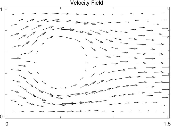 Figure 1
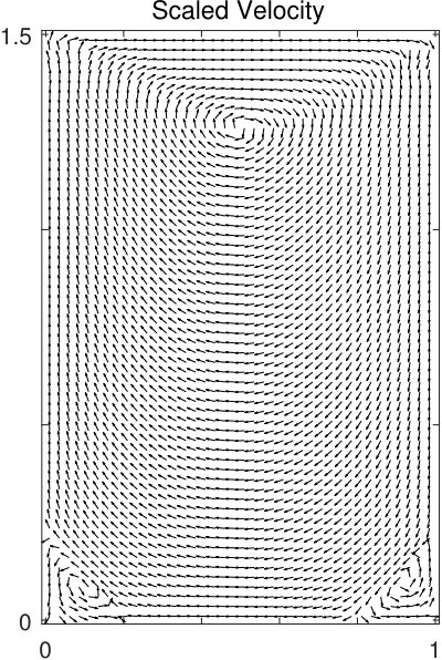 Figure 2
 Figure 3
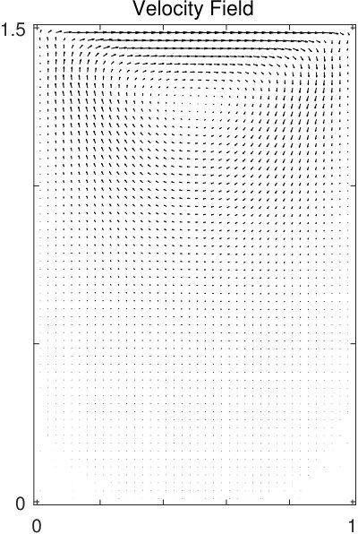 Figure 4
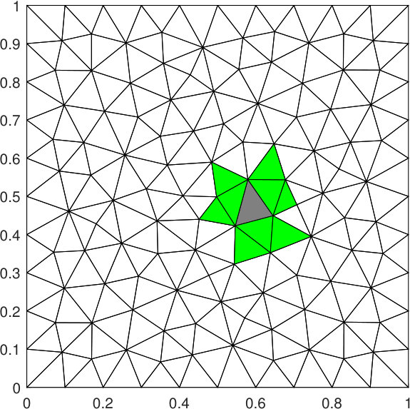 Figure 5
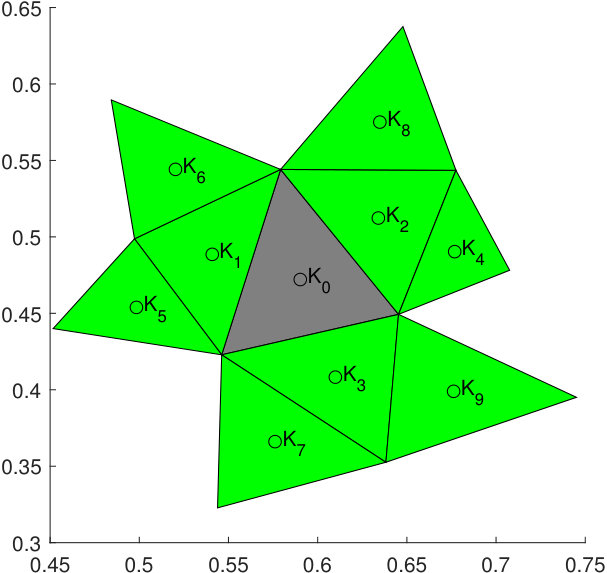 Figure 6
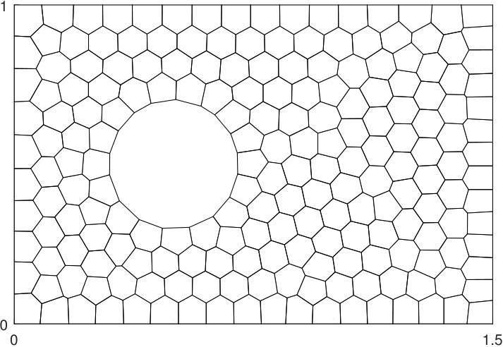 Figure 7
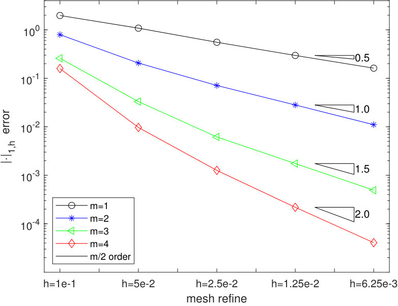 Figure 8
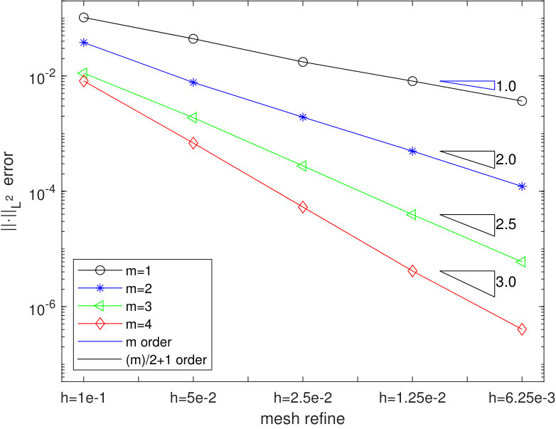 Figure 9
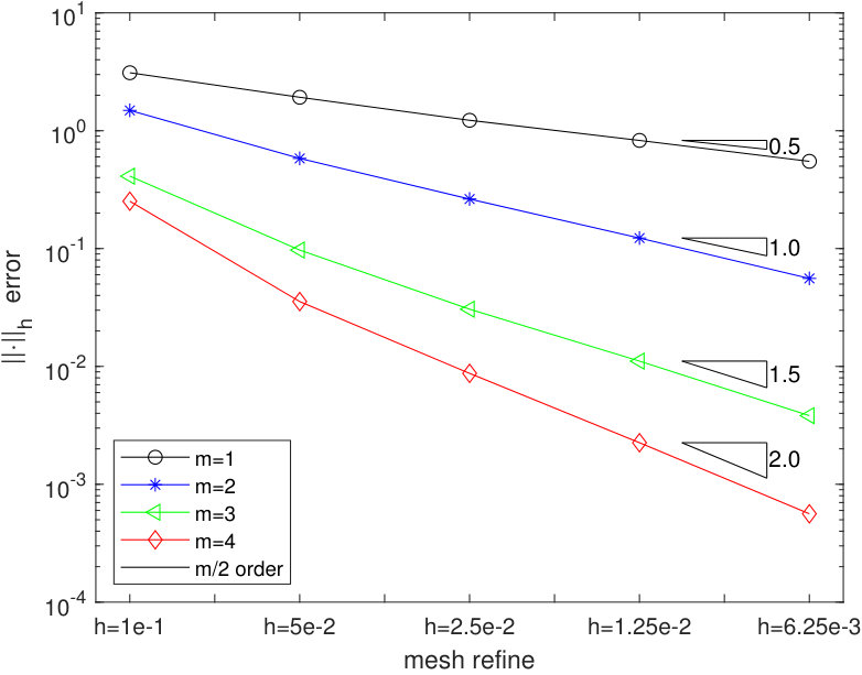 Figure 10
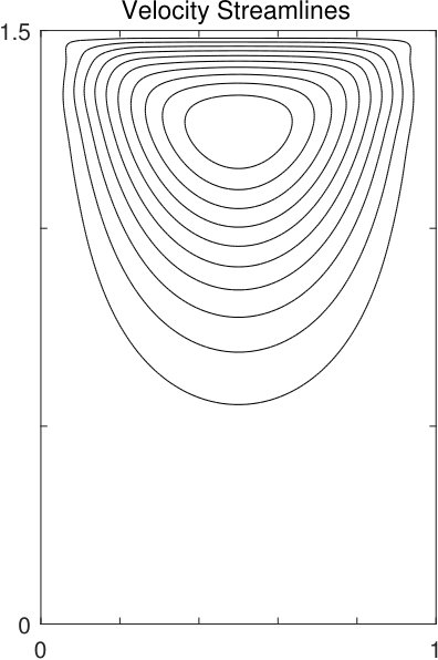 Figure 11
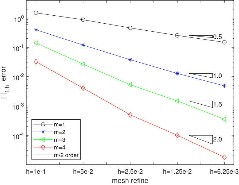 Figure 12
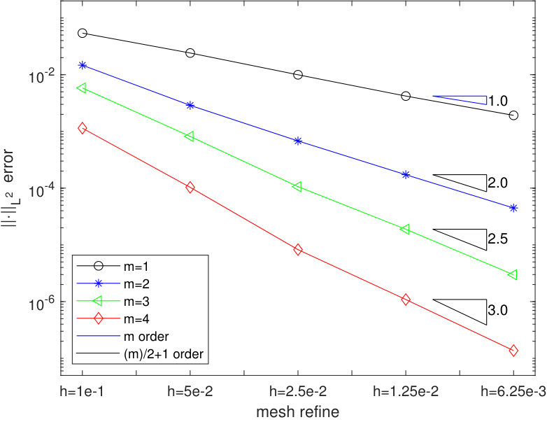 Figure 13
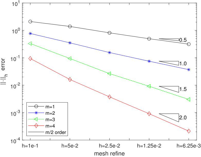 Figure 14
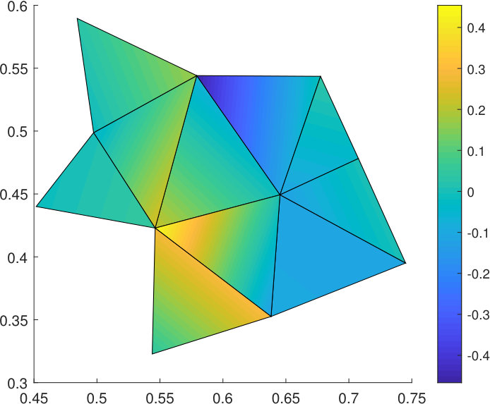 Figure 15
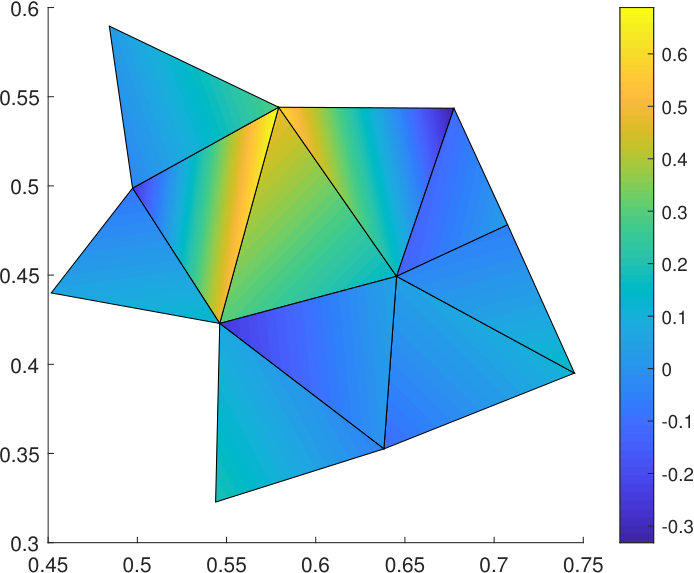 Figure 16
| h=1.0E-1 | 5.0E-2 | 2.5E-2 | 1.25E-2 | 6.25E-3 | ||||||
| Norm | error | error | order | error | order | error | order | error | order | |
| 5.41E-02 | 2.41E-02 | 1.16 | 9.97E-03 | 1.27 | 4.20E-03 | 1.24 | 1.92E-03 | 1.13 | ||
| 1.50E+00 | 8.76E-01 | 0.77 | 4.61E-01 | 0.92 | 2.55E-01 | 0.85 | 1.48E-01 | 0.77 | ||
| 1 | 2.10E+00 | 1.39E+00 | 0.59 | 8.16E-01 | 0.77 | 4.97E-01 | 0.71 | 3.15E-01 | 0.65 | |
| 1.47E-02 | 2.88E-03 | 2.34 | 6.79E-04 | 2.08 | 1.72E-04 | 1.97 | 4.47E-05 | 1.94 | ||
| 3.97E-01 | 1.19E-01 | 1.73 | 3.78E-02 | 1.66 | 1.28E-02 | 1.55 | 4.84E-03 | 1.40 | ||
| 2 | 7.72E-01 | 3.52E-01 | 1.13 | 1.55E-01 | 1.17 | 7.53E-01 | 1.04 | 3.71E-03 | 1.01 | |
| 5.84E-03 | 8.18E-04 | 2.83 | 1.06E-04 | 2.94 | 1.88E-05 | 2.49 | 2.97E-06 | 2.66 | ||
| 1.41E-01 | 2.67E-02 | 2.40 | 5.30E-03 | 2.33 | 1.48E-03 | 1.83 | 3.54E-04 | 2.06 | ||
| 3 | 3.33E-01 | 9.47E-01 | 1.81 | 2.66E-02 | 1.83 | 9.20E-03 | 1.53 | 3.04E-03 | 1.59 | |
| 1.14E-03 | 1.03E-04 | 3.46 | 8.25E-06 | 3.64 | 1.08E-06 | 2.92 | 1.36E-07 | 2.99 | ||
| 3.24E-02 | 4.06E-03 | 2.99 | 4.99E-04 | 3.02 | 9.96E-05 | 2.32 | 1.77E-05 | 2.48 | ||
| 4 | 9.44E-02 | 1.62E-02 | 2.54 | 3.76E-03 | 2.10 | 9.15E-04 | 2.04 | 2.12E-04 | 2.10 |
| h=1.0E-1 | 5.0E-2 | 2.5E-2 | 1.25E-2 | 6.25E-3 | ||||||
| Norm | error | error | order | error | order | error | order | error | order | |
| 1.03E-01 | 4.41E-02 | 1.22 | 1.74E-02 | 1.33 | 8.14E-03 | 1.10 | 3.67E-03 | 1.14 | ||
| 1.97E+00 | 1.08E+00 | 0.86 | 5.54E-01 | 0.96 | 2.96E-01 | 0.90 | 1.62E-01 | 0.87 | ||
| 1 | 3.10E+00 | 1.92E+00 | 0.69 | 1.22E+00 | 0.64 | 8.27E-01 | 0.56 | 5.50E-01 | 0.58 | |
| 3.80E-02 | 7.71E-03 | 2.30 | 1.92E-03 | 1.99 | 4.97E-04 | 1.95 | 1.21E-04 | 2.03 | ||
| 7.95E-01 | 2.06E-01 | 1.94 | 7.11E-02 | 1.53 | 2.81E-02 | 1.33 | 1.10E-02 | 1.35 | ||
| 2 | 1.48E+00 | 5.82E-01 | 1.35 | 2.63E-01 | 1.14 | 1.22E-01 | 1.10 | 5.58E-03 | 1.13 | |
| 1.11E-02 | 1.88E-03 | 2.56 | 2.75E-04 | 2.77 | 3.94E-05 | 2.80 | 5.96E-06 | 2.72 | ||
| 2.59E-01 | 3.31E-02 | 2.96 | 6.17E-03 | 2.42 | 1.74E-03 | 1.82 | 4.92E-04 | 1.82 | ||
| 3 | 4.11E-01 | 9.71E-02 | 2.08 | 3.06E-02 | 1.66 | 1.10E-02 | 1.46 | 3.82E-03 | 1.53 | |
| 8.18E-03 | 6.85E-04 | 3.57 | 5.32E-05 | 3.68 | 4.15E-06 | 3.68 | 4.04E-07 | 3.35 | ||
| 1.59E-01 | 9.69E-03 | 4.03 | 1.26E-03 | 2.94 | 2.18E-04 | 2.52 | 4.06E-05 | 2.42 | ||
| 4 | 2.52E-01 | 3.55E-02 | 2.82 | 8.73E-03 | 2.02 | 2.25E-03 | 1.95 | 5.62E-04 | 2.00 |
Peer Reviews
No public reviews on file for this paper yet. If you reviewed it on a platform where reviews are public (OpenReview, ICLR, NeurIPS, ICML), you can paste yours below so the community can read it here.
Videos
No videos yet. Explain this paper in a talk, walkthrough, or lecture? Add one.
A Discontinuous Galerkin Method for the Stokes
Equation by Divergence-free Patch Reconstruction
Ruo Li
CAPT, LMAM and School of Mathematical Sciences, Peking University, Beijing 100871, P.R. China
,
Zhiyuan Sun
School of Mathematical Sciences, Peking University, Beijing 100871, P.R. China
and
Zhijian Yang
School of Mathematics and Statistics, Wuhan University, Wuhan 430072, P.R. China
Abstract.
A discontinuous Galerkin method by patch reconstruction is proposed for Stokes flows. A locally divergence-free reconstruction space is employed as the approximation space, and the interior penalty method is adopted which imposes the normal component penalty terms to cancel out the pressure term. Consequently, the Stokes equation can be solved as an elliptic system instead of a saddle-point problem due to such weak form. The number of degree of freedoms of our method is the same as the number of elements in the mesh for different order of accuracy. The error estimations of the proposed method are given in a classical style, which are then verified by some numerical examples.
Keywords: discontinued Galerkin; patch reconstruction; Stokes equation; divergence-free; interior penalty
MSC2010: 65N30;76D07
1. Introduction
The incompressible Stokes equations describe the low Reynolds number flows which are the linearization of the Navier-Stokes equations [18]. In the finite element method for incompressible Stokes problem see, e.g. [8], the major concern is how to impose the incompressibility condition. The conforming mixed finite element methods are usually introduced weakly by the Lagrange multiplier, and solve a saddle points problem. The methods are required to setup the approximation spaces for velocity and pressure to satisfy the in-sup conditions, which is necessary to guarantee the numerical stability. Consequently, the numerical solution obtained is weakly divergence-free, we refer readers to [4] for more details.
The other approach to solve the incompressible Stokes equation is constructing a divergence-free space to automatically fulfill the incompressible condition and eliminate the pressure. There are many efforts on constructing global divergence-free basis function. For example, the Crouzeix-Raviart elements was proposed in [8], which are divergence-free in each element and continuous at the midpoint of element edges. The finite elements was proposed in [19]. The methods to construct these divergence-free spaces are quite subtle that it is a nontrivial job to extend these methods to a grid with its elements in unusual geometry. An alternative way is abandoning the normal continuity of basis function, and using the locally divergence-free elements which are proposed in [2]. See the recent developments in this fold in [11, 7, 16].
The discontinuous Galerkin (DG) method by patch reconstruction was recently introduced in [13] to solving the elliptic equation, then was developed in [12] and [15] to various model problems. We are motivated to approximate the divergence-free velocity in Stokes problem using the discontinuous space by patch reconstruction. Actually, we propose a locally divergence-free space by imposing the constrain locally in patch reconstruction. With the new space, we adopt the interior penalty method to Stokes problems [10]. The penalty term is introduced on the normal component to control the inconsistent error. Consequently, an elliptic problem is attained to be solved instead of a saddle-point problem. To construct the locally divergence-free space, we use the piecewisely solenoidal polynomial functions only. The space has one degree of freedom in each element. Therefore, the dimension of approximation space does not depend on the polynomial orders. The interpolation error estimate of this space can be obtained naturally, which leads to the approximate error estimate of the Stokes problem following the standard techniques. We note that the new space is a subspace of canonical locally divergence-free DG space. Our method enjoys the advantages of DG method, for example that it works on meshes with polygonal elements. We demonstrate by numerical examples on different meshes.
The rest of this paper is organized as follows. In Section 2, we describe the method to construct the locally divergence-free approximation space and and give the approximation estimate of this space. Then we present the interior penalty method of discontinued Galerkin method for Stokes problems in Section 3. The error estimate of the proposed method is obtained under the DG energy norm. Finally, numerical results for two-dimensional examples are presented in Section 4 to validate our estimates and demonstrate the capacity of our method.
2. Construction of Approximation Space
Let be a polygonal domain in . The mesh is a partition of with polygons denoted by that . For any two elements , , if . Here with the diameter of . We denote by the area of . denotes the union of boundaries of element , where is the union of interior boundaries . We assume that the partition possesses the following shape regularity conditions [5, 3]:
- A1
There exists an integer independent of , that any element admits a sub-decomposition which consists of at most triangles . 2. A2
is a compatible sub-decomposition, that any is shape-regular in the sense of Ciarlet-Raviart [6]: there exists a real positive number independent of such that , where is the radius of the greatest ball inscribed in .
Let to be a subdomain of , which may be an element or an aggregation of the elements belong to . Let demote the Sobolev space of real valued functions on with a positive integer . For vector valued functions, we introduce the spaces . Let be a set of polynomial with total degree not greater than on domain , and the corresponding vector valued polynomial spaces is denoted by .
Assumptions A1 and A2 allow quite general shapes in the partition, such as non-convex or degenerate elements. They also lead to some common used properties and inequalities:
- M1
, there exists that depends on and such that . 2. M2
[Agmon inequality] There exists a constant that depends on and , but independent of such that
[TABLE] 3. M3
[Approximation property] There exists a constant that depends on and , but independent of such that for any , there exists an approximation polynomial such that
[TABLE] 4. M4
[Inverse inequality] For any , there exists a constant that depends only on and such that
[TABLE] 5. M5
[Discrete trace inequality] For any , there exists a constant that depends only on and such that
[TABLE]
The above four inequalities (2.1), (2.2), (2.3) and (2.4) are hold for vector valued space and with corresponding norms,
[TABLE]
We are interested in the spaces of solenoidal vector fields
[TABLE]
and the polynomial solenoidal vector field
[TABLE]
The above inequalities are also hold for the and , see in [2]. Here we restate the approximation property:
M3 [Approximation property] There exists a constant that depends on and , but independent of such that for any , there exists an approximation polynomial such that
[TABLE]
In [13], we introduced the reconstruction operator which mapping the piecewise constant space to discontinuous piecewise polynomial space. In this paper, we intend to construct a reconstruction operator that embeds the piecewise constant vector valued space to discontinuous piecewise solenoidal vector fields. For each element , we assign a sampling node or collocation point and element patch . usually contains and some elements around . It is quite flexible to assign the sampling nodes and construct the element patch. Usually, we let the barycenter of the element to be the sampling node, while a perturbation is allowed, cf. [13]. The element patch is built up by adding Von Neumann neighbors (adjacent edge-neighboring elements) recursively until the size of the element patch reaches a fixed number, for the details we refer to [13, 14].
Let denote the set of the sampling nodes belonging to with denote its cardinality
[TABLE]
and let be the number of elements belonging to . These two numbers and are equal to each other. We define and .
Denote the piecewise constant space associated with by , i.e.,
[TABLE]
and let to be the piecewise constant vector valued space.
For any and for any , we reconstruct a high order solenoidal polynomials of degree by solving the following discrete least-square problem.
[TABLE]
Though gives a solenoidal approximation on the entire element patch , but we only use the approximation on the element . Then the reconstruction operator can extended to the function space , still denote by without ambiguity,
[TABLE]
where .
We make the following assumption on the sampling node set .
Assumption A For any and ,
[TABLE]
This assumption can guarantee the uniqueness of the solution of discrete least-square problem (2.6). Obvious, a necessary condition for the solvability of (2.6) is that is greater than . Assumption A is equal to the following quantitative estimate
[TABLE]
with
[TABLE]
If the mesh is quasi-uniform triangulation and each element patch is convex, the quantitative estimate of the uniform upper bound of for the general polynomial is obtained in [14]. The requirements of the uniform upper bound are hard to be satisfied while the polygonal meshes are applied. We refer the readers to [13] which gives the uniform upper bound under milder assumptions, such as polygonal partition and non-convex element patch. Due to the solenoidal polynomial space is the subspace of the general polynomial vector valued space, in (2.8) is uniformly bounded under the same assumption.
Lemma 2.1**.**
If Assumption A holds, then there exists a unique solution of (2.6), denoted by , for any . Moreover satisfies
[TABLE]
The stability property holds true for any and and as
[TABLE]
and the quasi-optimal approximation property is valid in the sense that
[TABLE]
where .
Proof.
The reconstruction operator is a projection operator from to with the discrete norm, the identity (2.9) is obvious.
By the Assumption A and definition of in equation (2.8),
[TABLE]
From the projection property of operator , we have
[TABLE]
Combining (2.12) and (2.13), we get
[TABLE]
Assume that is the best approximation of under norm, , and
[TABLE]
Then, we have following estimate:
[TABLE]
By triangle inequality, the left side of (2.11) can be written as
[TABLE]
Together with the definition of , it implies the quasi-optimality (2.11). ∎
Lemma 2.2**.**
If Assumption A holds and , then there exists a constant that depends on , and such that
[TABLE]
Proof.
By [2, Theorem 4.3], we take in the right-hand side of (2.11), where is the approximation solenoidal polynomial of order . Then
[TABLE]
where depends on and .
Substituting the above estimate (2.17) into (2.11), we obtain
[TABLE]
which gives (2.14).
Then, assume that be the approximation polynomial in (2.2) for function , by the inverse inequality (2.3) and the approximation estimate (2.14), then we have
[TABLE]
This gives (2.15).
Combing the Agmon inequality (2.1), (2.14) and (2.15), one has
[TABLE]
Taking the square root of both sides gives (2.16) completes the proof. ∎
A global reconstruction operator is defined by . Given , we embed into a piecewise discontinuous solenoidal polynomial finite element space with its order to be . The approximation space is defined by
[TABLE]
Furthermore, the reconstruction operator can be extended to function space , and we still denote by without ambiguity,
[TABLE]
where and .
The basis function of are given by the following process. Define to be the characteristic function corresponding to ,
[TABLE]
Let denote the basis function and it is defined by the reconstruction process:
[TABLE]
The reconstruction operator can be wrote explicitly with the given basis functions ,
[TABLE]
Next, we will show the implementation of the proposed method by an example on square domain . Here a third order solenoidal field reconstruction is considered, the basis functions of the corresponding solenoidal field are listed as follows,
[TABLE]
[TABLE]
[TABLE]
The total degree of freedoms of the third order solenoidal field is 14, it means the size of element patch at least need to be taken as 7 to guarantee the solvability of the least square problem. Thus we take as 10 and the barycenter as the sampling node. Figure 2.1 shows domain and the corresponding triangulation,
Here we take an element as a demonstration element, the element patch of is taken as
[TABLE]
and the corresponding set of the sampling nodes is
[TABLE]
The element patch and sampling nodes are shown in Figure 2.1.
For a given function , the least square problem (2.6) is as
[TABLE]
The problem is solved directly by calculating the generalized inverse of a matrix,
[TABLE]
where and are defined as follows
[TABLE]
is a matrix, limited by the page space, we only list the first order part, the rest is easy to be complemented. is a vector.
Matrix contains all the information of the basis functions that are defined on element , the matrix is relevant with . The basis function is determined after the reconstruction are conducted on each element. Figure 2.2 shows the basis function . We note that the support of is not equal to the element patch . Insteadly, for any element , the support of the basis function is related with all the element patches which includes :
[TABLE]
Due to the discontinuity of the reconstructed finite element space, the DG method can be directly employed. We end this section by introducing the average and jump operators which are common used in DG method. Let be an interior edge shared by two adjacent elements . The corresponding unit outward normal vector are denoted by , . Let and be the scalar valued and vector valued functions on , respectively. Following the traditional DG notations, we define the operator on element edges as follows:
[TABLE]
with . The operator on element edges is as
[TABLE]
For , we set
[TABLE]
3. Approximation of Stokes Equation
We consider the Stokes equation with Dirichlet boundary condition:
[TABLE]
where is the velocity field, is the pressure, and is the given boundary value satisfying the compatibility condition . We take the local divergence-free reconstruction space as the trial and test function spaces. The approximation problem of (3.1) is: Seek , such that
[TABLE]
where the bilinear form is defined by
[TABLE]
and
[TABLE]
*where and are penalty parameters, corresponding to different penalty term, respectively. *
We note that the weak form (3.2) is inconsistent [10]. Precisely, the solution of the equation (3.1) does not satisfy the weak form (3.2), saying
[TABLE]
The inconsistency is caused by the discontinuous of normal component on interior element edges. Instead of satisfying the weak form (3.2), satisfies
[TABLE]
Therefore, for the interior penalty scheme, the non-consistent penalty parameter need to be taken great enough to control the consistency error which is similar to the interior penalty method for elliptic equation [1]. Meanwhile, the penalty parameter is chosen to guarantee the stability of the operator . The magnitude of penalty parameters are taken as follows,
[TABLE]
where is the degree of polynomials in .
Let us define some mesh depended semi-norms, for ,
[TABLE]
and introduce the energy norm,
[TABLE]
By the results in the previous section, we instantly have following approximation estimate about energy norm,
Lemma 3.1**.**
For to be the solution of equation (3.1), and to be the interpolation of , there exists a constant that depends on , , and , such that
[TABLE]
Here we need to clarify that the approximation error is not optimal, which is due to the fact that the BDM space is not a subspace of the approximation space . The third term of energy norm is dominant in the approximation error. This fact makes the numerical solution not able to attain the optimal accuracy order.
For the consistency error, we have following estimate,
Lemma 3.2**.**
For and , we have
[TABLE]
Proof.
By Agmon inequality (2.1), we have
[TABLE]
∎
Next, the boundedness and the stability of the operator can be claimed as
Lemma 3.3**.**
For , , and sufficiently large and we have
[TABLE]
Now, with the above lemmas, we are ready to give the error estimate of the numerical solution (3.2),
Theorem 3.1**.**
For , to be the solution of equation (3.1), and to be the solution of equation (3.2), we then have
[TABLE]
Furthermore, the error estimate is as
[TABLE]
Proof.
We split the error with an interpolation function in ,
[TABLE]
Then together with the consistency error, we have
[TABLE]
From the stability of bilinear operator , the second term in (3.13) has
[TABLE]
Collecting the above estimates and Lemma 3.2, it gives
[TABLE]
The first term in (3.13) is the interpolation error,
[TABLE]
Collecting estimates (3.13) ,(3.16) and (3.17) together, we can have (3.11).
For the error estimate, we define the auxiliary functions and the adjoint problem
[TABLE]
then apply the test function , we have
[TABLE]
The regularity of Stokes equations implies
[TABLE]
where is the BDM interpolation function. This gives
[TABLE]
and
[TABLE]
Inserting (3.21) and (3.22) to the equation (3.19),
[TABLE]
Then substituting the energy norm estimate (3.11) into (3.23), the error estimate (3.12) is obtained. ∎
4. Numerical Examples
We present some numerical examples to illustrate the effectiveness of the proposed method. One merit of the method is the linear system is maintained with the given mesh while ignore the increase of approximation order. The maximum degree of approximation polynomial is taken as which is limited by the condition number of linear system. The numerical examples with various polygonal meshes are demonstrated. A direct solver is used to solve the linear algebra systems after discretisation.
4.1. Analytical example
This is an example with a smooth solution to verify the convergence order as the error estimate predicted. The Stokes problem with Dirichlet boundary condition is solved in two dimensional square domain . The exact velocity field and pressure are given as follows,
[TABLE]
The body force and boundary condition are given correspondingly. The quasi-uniform triangular and quadrilateral meshes are used, both of them are generated by the software gmsh[9].
Table 4.1 and 4.2 present the error of the numerical solution in norm, seminorm and norm. Figure 4.1 and 4.2 plot the accuracy order under different norm, respectively. The behavior of the proposed method agrees perfectly with the theoretical analysis on the convergence order to be on norm. And the convergence order of norm and seminorm are not optimal as usual situations, which are and , respectively. This is due to the fact that the space is not large enough that it can not contain the space as a subspace as the traditional discontinued Galerkin space. The difference between seminorm and norm error implies that the seminorm is dominate in energy norm. The condition number of resulting matrix is mainly determined by the penalty parameter . And the exponential growth of with the increasing of the degree of the polynomial results in very ill-posed linear system.
4.2. Lid-driven cavity example
The lid-driven cavity is a benchmark test for the incompressible flow that does not have an exact solution. Here we sets the cavity domain as a rectangle . The body force is zero, and a Dirichlet boundary condition is given as
[TABLE]
Figure 4.3 shows the velocity fields and the scaled velocity. The domain is segmented by a quasi-uniform triangle mesh meanwhile the third order polynomial is employed. The numerical results fit the realities. The scaled velocity present the expected phenomenon which the Contra vortices appear in the bottom corner. The subtle vortices will capture with refined mesh.
4.3. Flow around cylinder
Flow around cylinder is another representative benchmark test for the incompressible flow. The numerical setting is slightly different from the traditional setting. The polygonal elements are considered to demonstrate the compatibility of the proposed method. While the computational domain is a rectangle minus a circle , which is partitioned into polygonal elements mesh by PolyMesher [17]. The Dirichlet boundary condition is given while with zero body force.
[TABLE]
Figure 4.4 shows the polygonal mesh and the corresponding velocity field. The proposed method provides a smooth solution which is agreed with the expected behavior. and it can handle a wide variety of polygonal elements without additional techniques.
5. Conclusions
The discontinuous Galerkin method by locally divergence-free patch reconstruction for simulation of incompressible Stokes problems is developed. The interior penalty method with solenoidal velocity field allows calculating the velocity field with no presence of pressure. This method can achieve high order accuracy with one degree of freedom per element. In spite of such advantage, our method suffers from the inconsistence penalty term which leads to an ill-posed linear system for large .
The reference list from the paper itself. Each links out to its DOI / PubMed record.
- 1[1] D. N. Arnold, F. Brezzi, B. Cockburn, and L. D. Marini. Unified analysis of discontinuous Galerkin methods for elliptic problems. SIAM J. Numer. Anal. , 39(5):1749–1779, 2001/02.
- 2[2] G. A. Baker, W. N. Jureidini, and O. A. Karakashian. Piecewise solenoidal vector fields and the Stokes problem. SIAM J. Numer. Anal. , 27(6):1466–1485, 1990.
- 3[3] L. Beirão da Veiga, K. Lipnikov, and G. Manzini. The Mimetic Finite Difference Method for Elliptic Problems , volume 11 of MS&A. Modeling, Simulation and Applications . Springer, Cham, 2014.
- 4[4] D. Boffi, F. Brezzi, and M. Fortin. Mixed Finite Element Methods and Applications , volume 44 of Springer Series in Computational Mathematics . Springer, Heidelberg, 2013.
- 5[5] F. Brezzi, A. Buffa, and K. Lipnikov. Mimetic finite differences for elliptic problems. ESAIM Numer. Anal. , 43:277–295, 2009.
- 6[6] P. G. Ciarlet. The Finite Element Method for Elliptic Problems . North-Holland, Amsterdam, 1978.
- 7[7] B. Cockburn, G. Kanschat, and D. Schötzau. A note on discontinuous Galerkin divergence-free solutions of the Navier-Stokes equations. J. Sci. Comput. , 31(1-2):61–73, 2007.
- 8[8] M. Crouzeix and P.-A. Raviart. Conforming and nonconforming finite element methods for solving the stationary Stokes equations. I. Rev. Française Automat. Informat. Recherche Opérationnelle Sér. Rouge , 7(R-3):33–75, 1973.