Aerial navigation in obstructed environments with embedded nonlinear model predictive control
Elias Small, Pantelis Sopasakis, Emil Fresk, Panagiotis Patrinos,, George Nikolakopoulos

TL;DR
This paper introduces a real-time nonlinear model predictive control approach for autonomous aerial navigation and obstacle avoidance in complex environments, demonstrated on a micro aerial vehicle with embedded computation.
Contribution
It presents a novel NMPC methodology using PANOC for fast, embedded obstacle avoidance in non-convex environments, with a simple battery depletion compensation method.
Findings
NMPC with PANOC runs at 20Hz onboard MAV.
The MAV successfully navigates around obstacles smoothly.
Thrust compensation improves autonomy over time.
Abstract
We propose a methodology for autonomous aerial navigation and obstacle avoidance of micro aerial vehicles (MAV) using nonlinear model predictive control (NMPC) and we demonstrate its effectiveness with laboratory experiments. The proposed methodology can accommodate obstacles of arbitrary, potentially non-convex, geometry. The NMPC problem is solved using PANOC: a fast numerical optimization method which is completely matrix-free, is not sensitive to ill conditioning, involves only simple algebraic operations and is suitable for embedded NMPC. A C89 implementation of PANOC solves the NMPC problem at a rate of 20Hz on board a lab-scale MAV. The MAV performs smooth maneuvers moving around an obstacle. For increased autonomy, we propose a simple method to compensate for the reduction of thrust over time, which comes from the depletion of the MAV's battery, by estimating the thrust constant.
Click any figure to enlarge with its caption.
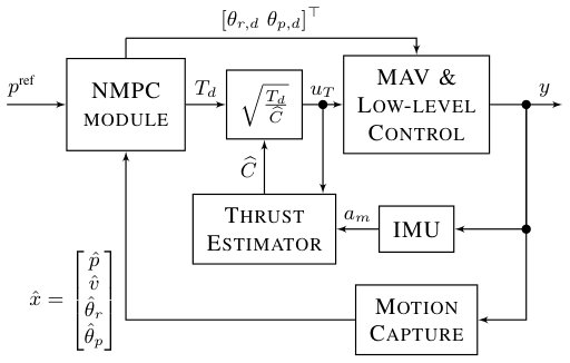 Figure 1
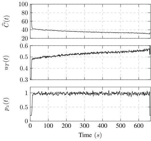 Figure 2
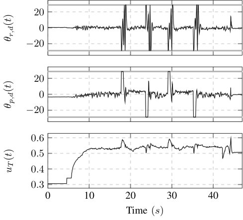 Figure 3
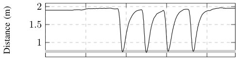 Figure 4
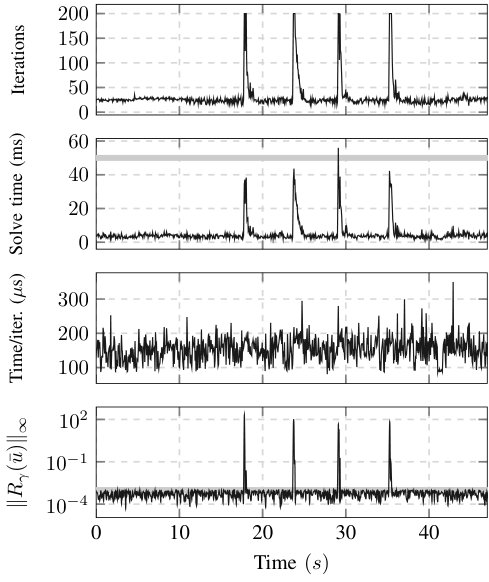 Figure 5
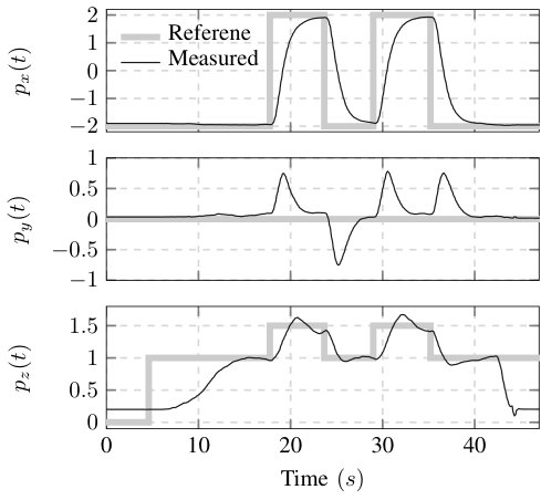 Figure 6
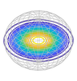 Figure 7
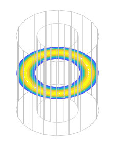 Figure 8
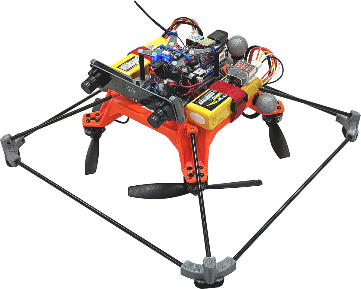 Figure 9
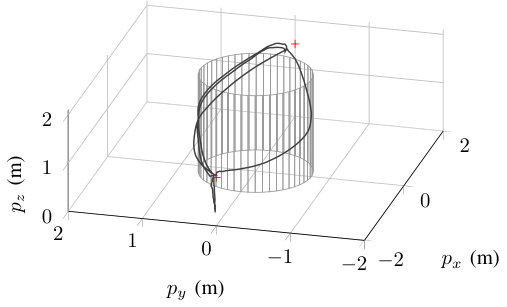 Figure 10
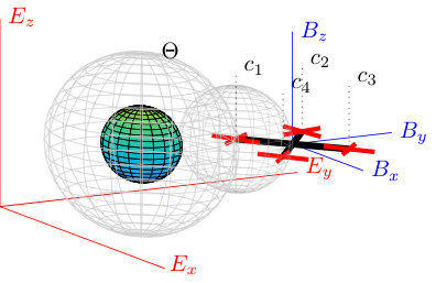 Figure 11
| parameter | value | parameter | value |
|---|---|---|---|
| 0.1 | 0.5 | ||
| 0.1 | 1 | ||
| 0.2 | 0.5 | ||
| 1 |
Peer Reviews
No public reviews on file for this paper yet. If you reviewed it on a platform where reviews are public (OpenReview, ICLR, NeurIPS, ICML), you can paste yours below so the community can read it here.
Videos
No videos yet. Explain this paper in a talk, walkthrough, or lecture? Add one.
Taxonomy
TopicsAdvanced Control Systems Optimization · Robotic Path Planning Algorithms · Adaptive Control of Nonlinear Systems
Aerial navigation in obstructed environments with
embedded nonlinear model predictive control
Elias Small, Pantelis Sopasakis, Emil Fresk, Panagiotis Patrinos and George Nikolakopoulos
P. Sopasakis is with University of Cyprus, Department of Electrical and Computer Engineering, KIOS Research Center for Intelligent Systems and Networks, 1 Panepistimiou Avenue, 2109 Aglantzia, Nicosia, Cyprus. [email protected]. E. Small, E. Fresk and G. Nikolakopoulos are with the Robotics Team at Luleå Technical University, Luleå SE-97187, Sweden elias.small, emil.fresk, [email protected]. Patrinos is with the Department of Electrical Engineering (Esat-Stadius), KU Leuven, Kasteelpark Arenberg 10, 3001, Leuven, Belgium. [email protected] work was partially funded by the European Union’s Horizon 2020 Research and Innovation Programme under Grant Agreement No.730302 – SIMS. P. Sopasakis was supported by European Union’s Horizon 2020 research and innovation programme (KIOS CoE) under Grant No. 739551. P. Patrinos was supported by: FWO projects: No. G086318N; No. G086518N; Fonds de la Recherche Scientifique — FNRS, the Fonds Wetenschappelijk Onderzoek — Vlaanderen under EOS Project No. 30468160 (SeLMA) and Research Council KU Leuven C1 project No. C14/18/068.
Abstract
We propose a methodology for autonomous aerial navigation and obstacle avoidance of micro aerial vehicles using non-linear model predictive control (NMPC) and we demonstrate its effectiveness with laboratory experiments. The proposed methodology can accommodate obstacles of arbitrary, potentially non-convex, geometry. The NMPC problem is solved using PANOC: a fast numerical optimization method which is completely matrix-free, is not sensitive to ill conditioning, involves only simple algebraic operations and is suitable for embedded NMPC. A C89 implementation of PANOC solves the NMPC problem at a rate of on board a lab-scale MAV. The MAV performs smooth maneuvers moving around an obstacle. For increased autonomy, we propose a simple method to compensate for the reduction of thrust over time, which comes from the depletion of the MAV’s battery, by estimating the thrust constant.
I Introduction
I-A Background and motivation
The need for safe aerial navigation and increased MAV autonomy nowadays poses all the more relevant and pressing research questions, as drones make their appearance in numerous application domains, such as the inspection of critical or aging infrastructure [1], surveying of underground mines [2], visual area coverage for search-and-rescue operations [3], precision agriculture [4] and many others. In the majority of these applications, MAVs have to navigate in obstructed environments, with static or moving obstacles of arbitrary geometry in known, or partially unknown surrounding environments.
Several methods have been proposed for navigation and collision avoidance, such as potential field methods [5, 6] and graph search methods [7]. Alongside these methods, NMPC is becoming popular for the navigation control of various MAVs including fixed-wing aircrafts [8, 9] and multi-rotor vehicles [10]. NMPC uses a nonlinear dynamical model of the system dynamics to predict position and attitude trajectories from its current position to a reference point, while avoiding all obstacles on its way and minimizing a certain energy/cost function. In this way, a non-convex optimization problem needs to be solved at every sampling time instant in a receding horizon fashion. Another approach to obstacle avoidance is described in [11] where a high-level path planner generates collision-free trajectories which are followed by an MPC controller.
In [12], sequential quadratic programming (SQP) is used to solve the NMPC problem for the navigation of a multi-rotor MAV with a slung load, where the authors demonstrated the effectiveness of NMPC, however, provided neither evidence of the solution quality or solver performance, nor an experimental verification. NMPC was used in [13] for solving obstacle and collision avoidance for several MAVs flying in formation, however again, only simulations were done and the computation time was addressed.
Clearly, the presence of obstacle/collision avoidance constraints makes the MPC problems particularly hard to solve. SQP is the method of choice in the literature [12, 13, 14] that has as a main disadvantage the fact that it requires the solution of a quadratic program (QP) at every iteration of the algorithm, which requires inner iterations. SQP also requires computing and storing of the Jacobian matrices of the dynamics, and sometimes the Hessians when the Hessian of the Lagrangian is used in the QPs. Furthermore, the gradient descent method has been used to solve nonlinear MPC problems for aerial navigation [14]. This method, however, is sensitive to bad conditioning and problems with long horizons tend to become ill conditioned, while the convergence is expected to be slow.
I-B Contributions
In this article we propose a control methodology for the autonomous navigation of MAVs in obstructed environments. We allow for the obstacles to have arbitrary non-convex shapes and, contrary to distance-based methods [15], we do not require that the distance function between the MAVs and each obstacle is available.
The NMPC optimization problem is solved by using PANOC [16, 17] — a recently proposed algorithm for non-convex optimization problems, which is suitable for embedded NMPC, as it requires only simple and cheap linear operations (mainly inner products of vectors) and exhibits a fast convergence. Unlike SQP, PANOC is matrix-free and only requires the computation of Jacobian-vector products, which can be computed very efficiently by backward (adjoint) automatic differentiation. PANOC has been shown in [16, 17, 18] to significantly outperform both SQP and interior-point methods. To the authors best of knowledge, this is the first time that a fast NMPC optimization problem is being demonstrated on an aerial platform, setting the base for future developments in the aerial robotics community.
Our method for modeling has the strong merit of being independent of the mass of the MAV, whereas the norm in the community is to use mass and other detailed parameters of the specific MAV used, for example [10], [11], and [13]. This allows for our method to be used without tuning the specific mass or available thrust, improving robustness, generalization and ease of use.
Evidence of the solution quality is provided by physical laboratory experiments, where a MAV is flown completely autonomously in a laboratory equipped with a VICON motion capture system. The proposed method uses a full position and attitude model of the MAVs, which is able to run onboard, using 8-15% CPU of a single core on an Intel Atom Z8350. As is shown in Section V the onboard controller is able to successfully navigate the MAV around an obstacle running at a sampling rate of and a prediction horizon of .
II MAV dynamics
II-A MAV* kinematics*
The model of a quadrotor MAV, defined by [9], assumes that there exists a low-level controller of roll, pitch, yaw rate and thrust. This convention is common in MAV flight controllers such as PixHawk, [19] and ROSFlight, [20]. The high-level kinematics of the MAV is given by
[TABLE]
where and are the position and velocity of the MAV in the global frame of reference, and and are the roll and pitch angles, while and are the reference angles sent to the low-level controller. Furthermore, is the -axis thrust acceleration, while , , and are the linear drag coefficients. The lower layer — the attitude control system — is modeled by simple first-order dynamics with time constant and and gains and for the roll and pitch respectively. Lastly, describes the MAV’s attitude and is defined by the classical Euler angles in rotation matrix form as
[TABLE]
with
[TABLE]
Note that yaw is absent in this rotation matrix, as this model operates in a yaw-compensated global frame, and the position control of the MAV is therefore independent of its yaw. Moreover, it is important to note that we have chosen the acceleration, , to be the manipulated variable of the system, rather than the corresponding force, for the model to be mass-free. This has the strong merit of making the controller robust to changes in the mass of the MAV, the available thrust from the motors, and the loss of thrust over time due to the decline of battery voltage.
II-B Adaptive acceleration control
In order for our design to be independent of the physical characteristics that determine the available thrust acceleration, a simplified version of [21] is used to continuously estimate the MAV’s maximum available thrust. Following [21], the force, , that is exercised by the propellers, is given by
[TABLE]
where is the thrust constant and is a unitless normalized thrust control signal. The thrust constant is time dependent based, for instance, on battery drain and how close the MAV is to the ground, which is why identifying a constant is not sufficient to track thrust references. The issue is that there is no sensor in the system, which measures the generated force, however, the IMU can provide a measurement of the linear acceleration, albeit noisy. Then, by dividing the thrust model by the mass of the MAV, , the model is now based on acceleration:
[TABLE]
Equations (1ca) and (1cb) define a nonlinear dynamical system with state variable , input and output . We estimate by means of an extended Kalman filter (EKF). EKF is chosen because it is simple to tune, it allows to specify an initial estimate variance, and converges fast in the first few iterations.
In additional, we employ an outlier rejection scheme based on bounds of the direct estimate , where
[TABLE]
which is calculated for each IMU acceleration measurement , which implies that each acceleration measurement is inspected to enforce that no outliers are allowed to update the filter. These bounds result from the fact that a MAV must be able to generate at least of thrust to take off and it is assumed that it cannot generate more than of thrust. The bounds on are inherited by the estimates yielding a simple constrained estimation scheme.
Once the thrust constant is estimated, an acceleration reference can be converted to the thrust control signal , by solving equation (1ca) for , resulting in
[TABLE]
A depiction of how the thrust constant estimation is tied to the overall scheme can be found in Fig. 1.
II-C Overall system dynamics
The state of the controlled system is defined to be and the manipulated input is . The system is observed using a VICON motion capture system, which measures the full odometry of the system and provides the corresponding estimates of the full state of the MAV as . Overall, the system dynamics can be concisely written as
[TABLE]
where is implicitly defined via (1).
III Nonlinear MPC for obstacle avoidance
III-A Navigation in obstructed environments
We assume that a MAV needs to navigate towards a reference position , while avoiding a set of moving obstacles .
We select corner points on the MAV and position a ball with radius centered at each such point so that the whole vehicle is contained in the union of these balls. We assume that the coordinates of the corner points in the global frame of reference are given by , for .
In order for the MAV to not collide with the obstacles, we shall require that
[TABLE]
for all , , where is a ball centered at the origin with radius . The set is an enlarged version of the original obstacle . The concept is illustrated in Fig. 2.
We introduce the stage cost function and the terminal cost function which penalize the deviation of the system state from a reference state. Typical choices are
[TABLE]
where , and are positive semi-definite matrices and is the reference state which has the form .
The nonlinear model predictive control problem for navigation in an obstructed environment consists in solving the following problem
[TABLE]
where and , for are the predicted input and state signals.
In this formulation we have assumed that the future trajectories of all obstacles are exactly known and independent of the trajectory of the controlled vehicle. If this is not the case, we have to formulate appropriate robust or stochastic variants of the above obstacle avoidance problem.
The control action is exercised to the system via a zero-order hold element, that is, for , where is the sampling period. We assume that for some . Then, the cost function in (1ia) can be written as
[TABLE]
Since it is not possible to derive analytical solutions of the nonlinear dynamical system (1ic), the system trajectories as well as the cost function along these trajectories has to be evaluated by discretizing the system dynamics and integrals. By doing so, the system state trajectoriy is evaluated at points as follows
[TABLE]
and
[TABLE]
Any explicit integration method such as the fourth-order Runge-Kutta or Forward Euler lead to high quality approximations of MAV trajectories. This way, the original continuous-time optimal control problem is approximated by a discrete-time one which is solved at every time instant in a receding horizon fashion.
III-B Penalty functions for obstacles of general shape
Each obstacle is described by a set of nonlinear constraints of the form
[TABLE]
where functions are functions. This approach allows one to describe obstacles of very general convex or nonconvex shape. For example, by choosing functions to be affine in , we can model any polytopic object. Functions of the form can be used to model ellipsoidal objects or elliptic cylindrical ones. Polynomial, trigonometric and other functions can be used to model more complex geometric shapes.
For simplicity, in this section we focus in the case where there is one obstacle, that is , which we denote by . The constraint is satisfied if and only if for some , or equivalently, if
[TABLE]
for all , where is the function defined as
[TABLE]
Such a function is illustrated in Fig. 3. Function takes the value [math] outside the enlarged obstacle and increases in the interior of it as we move away from its boundary.
Function is differentiable with gradient
[TABLE]
where is the characteristic function of with if and otherwise.
Functions can be used to impose the obstacle avoidance requirements as soft constraints. To this end, we eliminate the non-convex constraints and introduce the modified stage and terminal cost functions
[TABLE]
where and are positive weight coefficients. The overall model predictive control (MPC) problem becomes
[TABLE]
The optimization is carried out over finite-dimensional vectors with .
III-C Single-shooting problem formulation
We shall cast optimization problem (1o) in the following compact and simple form
[TABLE]
where and is a function. To this end, we need to eliminate the state sequence in (1oc). Let us introduce a sequence of functions for defined recursively by
[TABLE]
Then, problem (1o) is written as in (1p) with
[TABLE]
This is known as the single shooting formulation [16].
IV Fast online nonlinear MPC using PANOC
Problem (1p) is in a form that can be solved by PANOC [16]. In particular, the gradient of can be computed using automatic differentiation [22] which is implemented by software such as CasADi [23]. PANOC finds a which solves the optimality conditions
[TABLE]
where is the fixed-point residual operator with parameter defined as
[TABLE]
where is the projected gradient operator given by
[TABLE]
PANOC combines safe projected-gradient updates with fast Newton-type directions computed by L-BFGS while it uses the forward backward envelope (FBE) function as a merit function for globalization given by
[TABLE]
The forward-backward envelope is an exact, continuous and real-valued merit function which shares the same (local/strong) minima with (1p). That said, Problem (1p) is reduced to the unconstrained minimization of .
PANOC is shown in Algorithm 1. L-BFGS uses a buffer of length of vectors and to compute the update directions [16], [24, Sec. 7.2]. The computation of requires only inner products which amount to a maximum of scalar multiplications. In particular, following [25], the L-BFGS buffer is updated only if .
Overall, PANOC uses exactly the same oracle as the projected gradient method, that is it only requires the invocation of , and . Lastly, owing to the FBE-based line search, PANOC converges globally, that is, from any initial guess, .
V Experimental validation
For the experimental validation of the proposed control scheme, an inverted quadrotor using the ROSFlight [20] low-level controller was used for all trials, shown in Fig. 4. The onboard computer used is an Aaeon Up Board with an Intel Atom x5-z8350 processor with four cores and of RAM. The board runs Ubuntu Server 16.04. The field robotics lab at LuleåUniversity of technology is equipped with a Vicon motion capture system featuring 20 infrared cameras that track the odometry of the MAV; this data is used by the NMPC controller for navigation.
The NMPC module runs simple C89 code which was generated by nmpc-codegen — an LGPLv3.0-licensed open-source code generation toolkit which is available at github.com/kul-forbes/nmpc-codegen.
An upright cylindrical obstacle, , is placed so that its vertical symmetry axis runs through the origin of the global coordinate frame in the flying arena at field robotics lab (FROST). The cylinder, , has a radius of and height . The obstacle is described by the functions , and . A single corner point is used which is positioned at the center of the MAV; the enclosing ball as in Fig. 2 has a radius of . In order to account for possible small constraint violations due to the fact that obstacle avoidance constraints are modeled via penalty functions, we consider an additional enlargement of . As a result, the enlarged cylinder, , has a radius of and height . The weights of the obstacle constraints, and , in Equation (1n) were all set to , and the continuous-time system was integrate with the forward Euler method.
The flight test performed for avoiding the obstacle consisted of alternating between two position references on opposite sides of the obstacle. The two position references given alternately were, in meters, and . These references were sent when the MAV was close to its previous reference position. The exact time the references are changed can be seen in Fig. 6.
NMPC runs at with a prediction and control horizon of 40 steps, meaning the solver predicts the states of the system into the future. The solver occupied between and of CPU on an Intel Atom Z8350 — an indication of the solver’s computational efficiency.
Fig. 5 shows the actual path flown by the MAV during the test where the positioning data is taken from the motion tracking system and has sub-millimeter accuracy. The path is also shown in Fig. 6 where we plot the MAV’s position versus time. The MAV does not have time to settle at the reference altitude as a new reference is sent to the controller before the position completely converges.
As the MAV passes the obstacle it violates the obstacle constraint, as shown in Fig. 7, which is expected from the penalty formulation. The maximum violation is , which is below the extra enlargement of of the obstacle.
Fig. 8 shows the control signals (roll, pitch, and normalized thrust references) commanded by the NMPC. The roll and pitch angles are bound between and ; these bounds are active as shown in Fig. 8. This further motivates the use of NMPC, allowing for bounds to be directly included in the problem formulation.
The control signals could be made less aggressive by penalizing the rate of change of the input in (1o), that is, by adding a penalty of the form for a symmetric positive semidefinite matrix . Nevertheless, the maneuvering of the MAV is smooth as shown in Figs. 5, 6 and 7 and a video of the experiment which can be found at https://youtu.be/E4vCSJw97FQ.
As shown in the second subfigure of Fig. 9, once the reference changes, the solver reaches the maximum number of iterations (200 iterations) and the solution it returns is of poor quality (fourth subfigure of Fig. 9). This happens because at each time instance, the solver is initialized with the previously computed optimal trajectory. Upon a reference change, the initial guess is rather far from optimal and this necessitates more iterations for convergence. Nonetheless, this inaccuracy is eliminated at the next time instant — later — where the solver is provided a good initial estimate and converges within the prescribed tolerance, . This way, NMPC is executed at . As shown in the third subfigure of Fig. 9, at one time instant, the solution time exceeds the maximum allowed time. This is accommodated by delaying the dispatch of the control action by few and has no practical effect.
The infinity norm of the fixed-point residual is below at all time instants with the exception of four instants from the change of reference. Lastly, the average iteration time in every time step is shown in the third subfigure of Fig. 9, and ranges from to where the variability is because of the different number of line search iterations.
The parameters used in the dynamics of the MAV used in the experiment are shown in Table I. These values were chosen empirically (based on accurate values for other MAVs) and are not fine-tuned via experiments; this accentuates the fact that the closed-loop and the overall obstacle avoidance scheme is robust to errors in the determination of these parameters.
The tuning parameters used by the NMPC are
[TABLE]
and the prediction horizon . For the EKF for estimating the special thrust constant we have
[TABLE]
where is the initial variance for , is the process variance in (1cb), and is the measurement variance.
A separate experiment was carried out where the MAV was given a position reference to hold for as long as the battery could deliver power safely. This experiment was conducted to demonstrate the thrust constant estimation described in Section II-B and the results are presented in Fig. 10. As the battery drains, the special thrust constant is decreasing and the control signal is adapted to keep the MAV hovering at a constant altitude. This experiment is part of the same video mentioned in this section, found at https://youtu.be/E4vCSJw97FQ.
VI Conclusions
We presented an obstacle and collision avoidance methodology coupled with an adaptive thrust controller that leads to increased autonomy and context awareness for MAVs. Obstacle avoidance is addressed with an NMPC controller, which is solved using PANOC — a simple and fast algorithm, which involves simple algebraic operations and, unlike SQP, does not require the solution of linear systems at each step. Experiments were performed with the solver running onboard a MAV which maneuvered gently around a virtual obstacle with a smooth trajectory. The MAV passed the edge of the virtual obstacle with a minimal constraint violation, as expected from the solver.
Moreover, experiments were performed to demonstrate that our thrust estimation method successfully compensates for the reduction of thrust over time, making the control scheme applicable to any MAV platform.
Future work will focus on experiments in presence of moving obstacles with uncertain trajectories.
The reference list from the paper itself. Each links out to its DOI / PubMed record.
- 1[1] N. Metni and T. Hamel, “A UAV for bridge inspection: Visual servoing control law with orientation limits,” vol. 17, no. 1, pp. 3 – 10, 2007.
- 2[2] C. Kanellakis, S. S. Mansouri, G. Georgoulas, and G. Nikolakopoulos, “Towards autonomous surveying of underground mine using MA Vs,” in Advances in Service and Industrial Robotics , N. A. Aspragathos, P. N. Koustoumpardis, and V. C. Moulianitis, Eds. Springer International Publishing, 2019, pp. 173–180.
- 3[3] S. S. Mansouri, C. Kanellakis, G. Georgoulas, D. Kominiak, T. Gustafsson, and G. Nikolakopoulos, “2D visual area coverage and path planning coupled with camera footprints,” vol. 75, pp. 1 – 16, 2018.
- 4[4] C. Zhang and J. M. Kovacs, “The application of small unmanned aerial systems for precision agriculture: a review,” vol. 13, no. 6, pp. 693–712, Dec 2012.
- 5[5] J. Minguez, F. Lamiraux, and J.-P. Laumond, Motion Planning and Obstacle Avoidance . Springer, 2016, pp. 1177–1202.
- 6[6] O. Montiel, U. Orozco-Rosas, and R. Sepúlveda, “Path planning for mobile robots using bacterial potential field for avoiding static and dynamic obstacles,” vol. 42, no. 12, pp. 5177–5191, 2015.
- 7[7] X. Chen and X. Chen, “The UAV dynamic path planning algorithm research based on Voronoi diagram,” in The 26th Chinese Control and Decision Conference (2014 CCDC) , May 2014, pp. 1069–1071.
- 8[8] T. J. Stastny, A. Dash, and R. Siegwart, “Nonlinear MPC for fixed-wing UAV trajectory tracking: Implementation and flight experiments,” in AIAA Guidance, Navigation, and Control Conference . American Institute of Aeronautics and Astronautics, jan 2017.