Hyperuniformity on spherical surfaces
Ariel G. Meyra, Guillermo J. Zarragoicoechea, Alberto. L. Maltz,, Enrique Lomba, Salvatore Torquato

TL;DR
This paper investigates hyperuniform point distributions on spherical surfaces, analyzing local particle number variance to characterize order and disorder, extending hyperuniformity concepts from Euclidean to curved geometries.
Contribution
It introduces a method to characterize hyperuniformity on spherical surfaces using local number variance scaling, addressing a gap in existing literature.
Findings
Hyperuniformity can be characterized on spherical surfaces via number variance scaling.
Disordered hyperuniform systems like avian retina photoreceptors are analyzed.
The approach applies to regular, uniform, and equilibrium particle configurations.
Abstract
In this work we present a study on the characterization of ordered and disordered hyperuniform point distributions on spherical surfaces. In spite of the extensive literature on disordered hyperuniform systems in Euclidean geometries, to date few works have dealt with the problem of hyperuniformity in curved spaces. As a matter of fact, some systems that display disordered hyperuniformity, like the space distribution of photoreceptors in avian retina, actually occur on curved surfaces. Here we will focus on the local particle number variance and its dependence on the size of the sampling window (which we take to be a spherical cap) for regular and uniform point distributions, as well as for equilibrium configurations of fluid particles interacting through Lennard-Jones, dipole-dipole and charge-charge potentials. We will show how the scaling of the local number variance enables the…
Click any figure to enlarge with its caption.
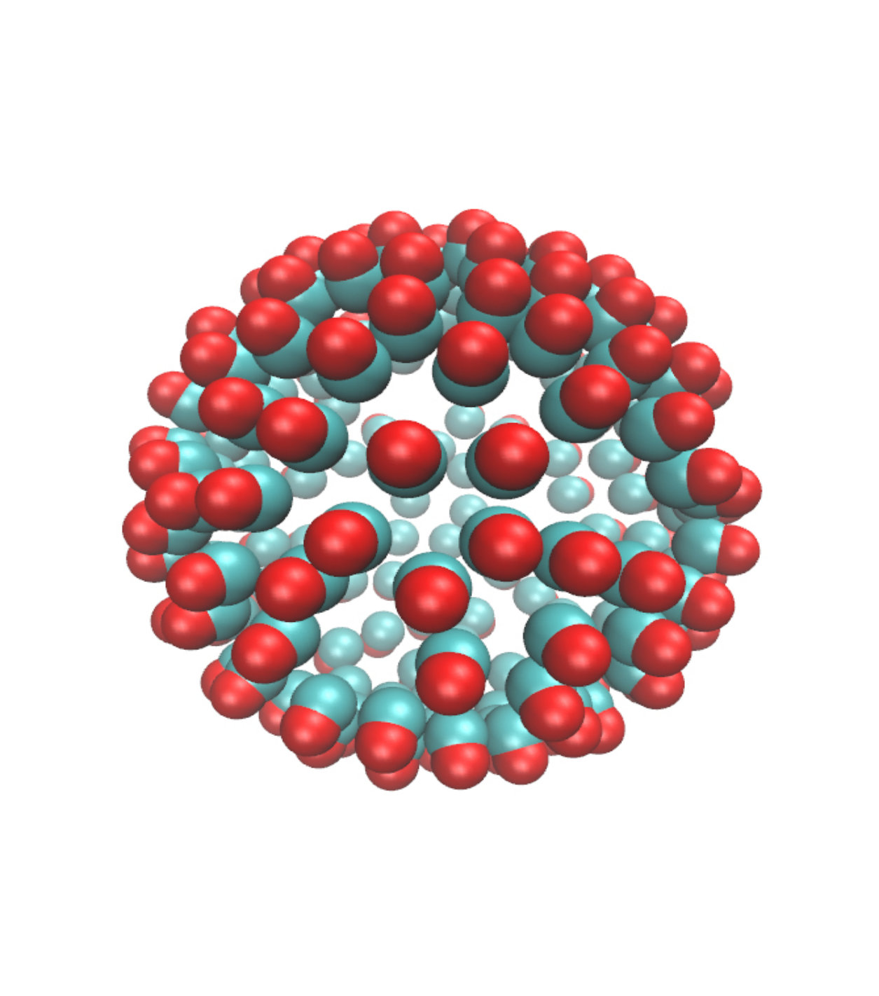 Figure 1
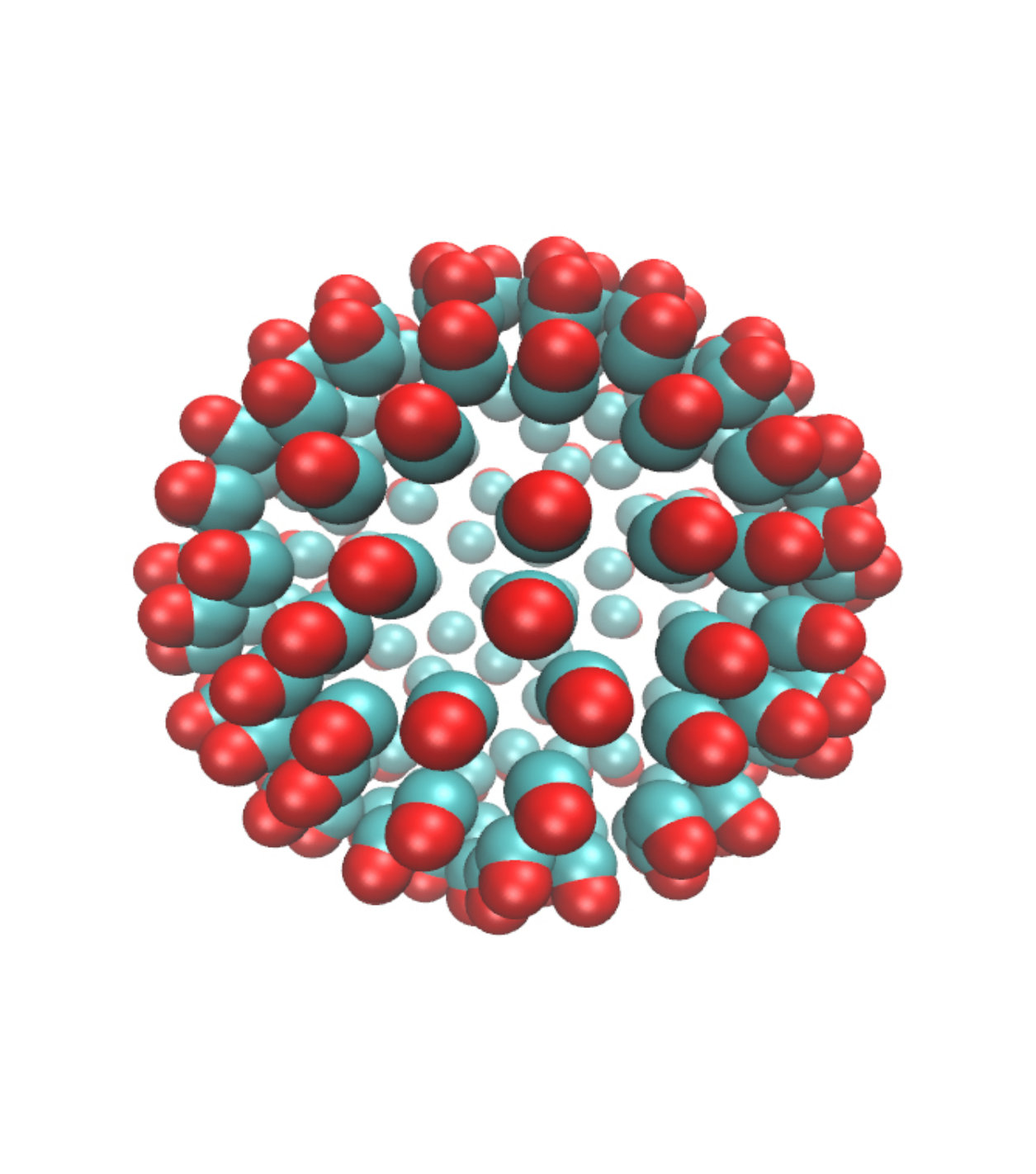 Figure 2
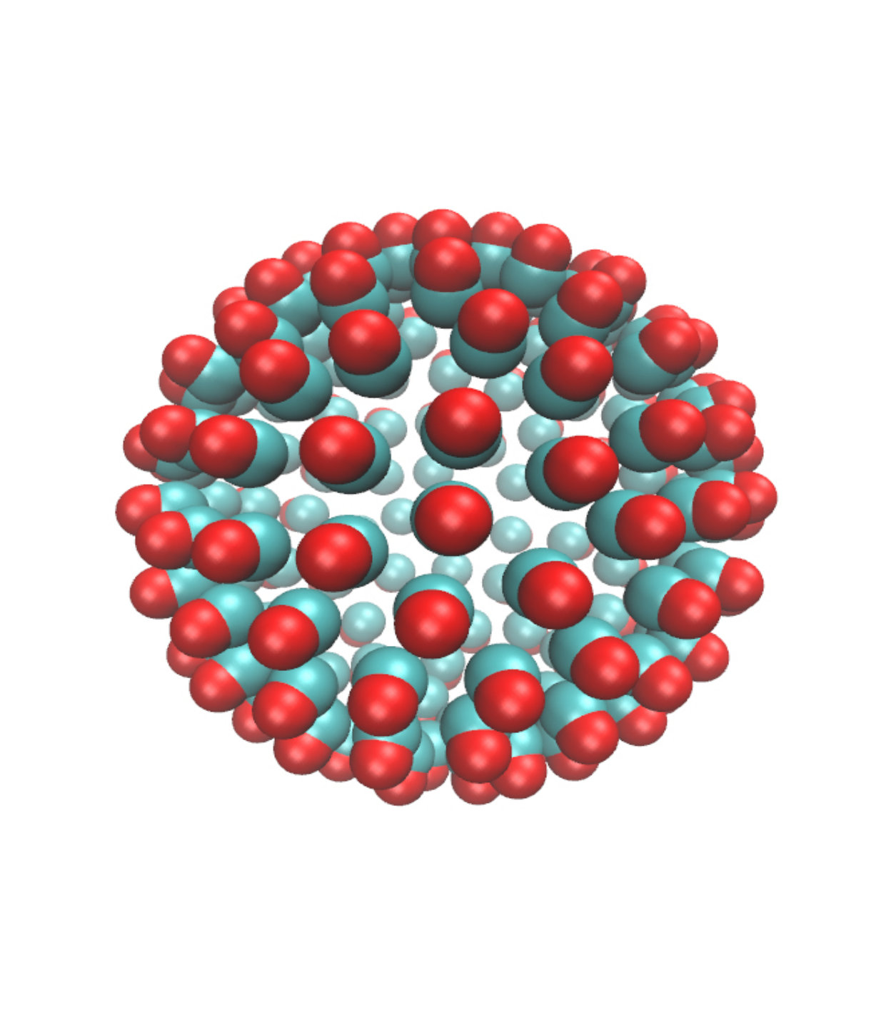 Figure 3
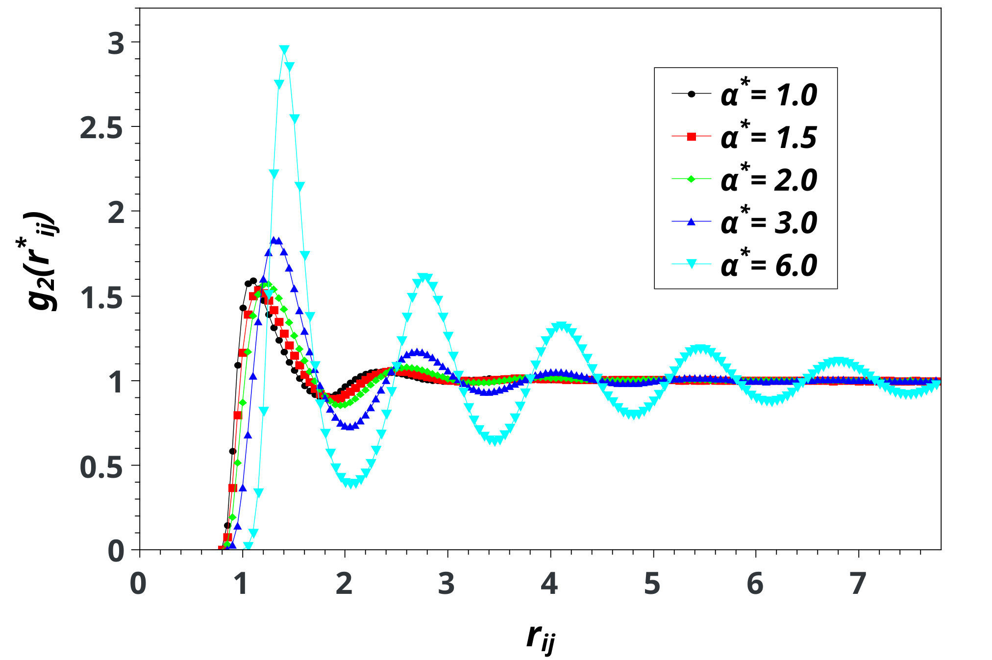 Figure 4
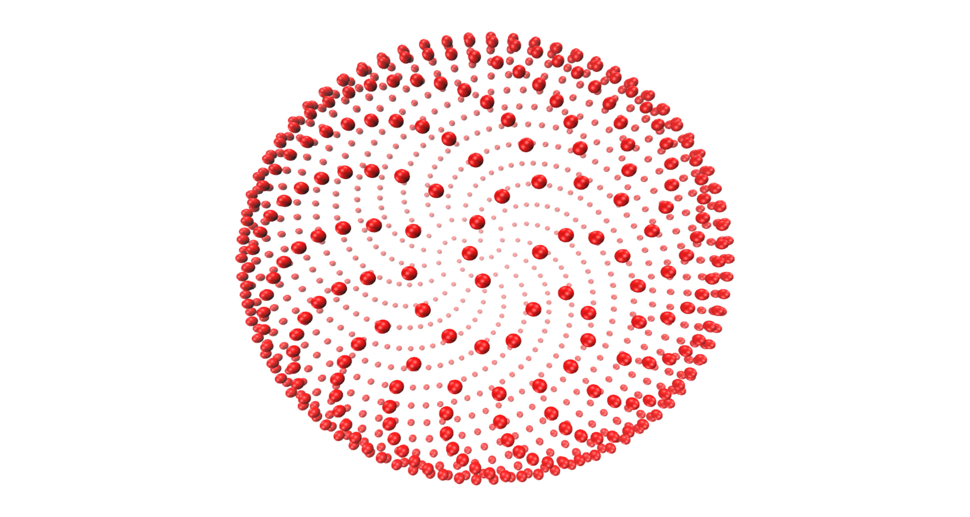 Figure 5
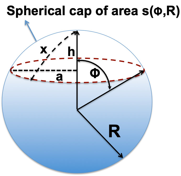 Figure 1
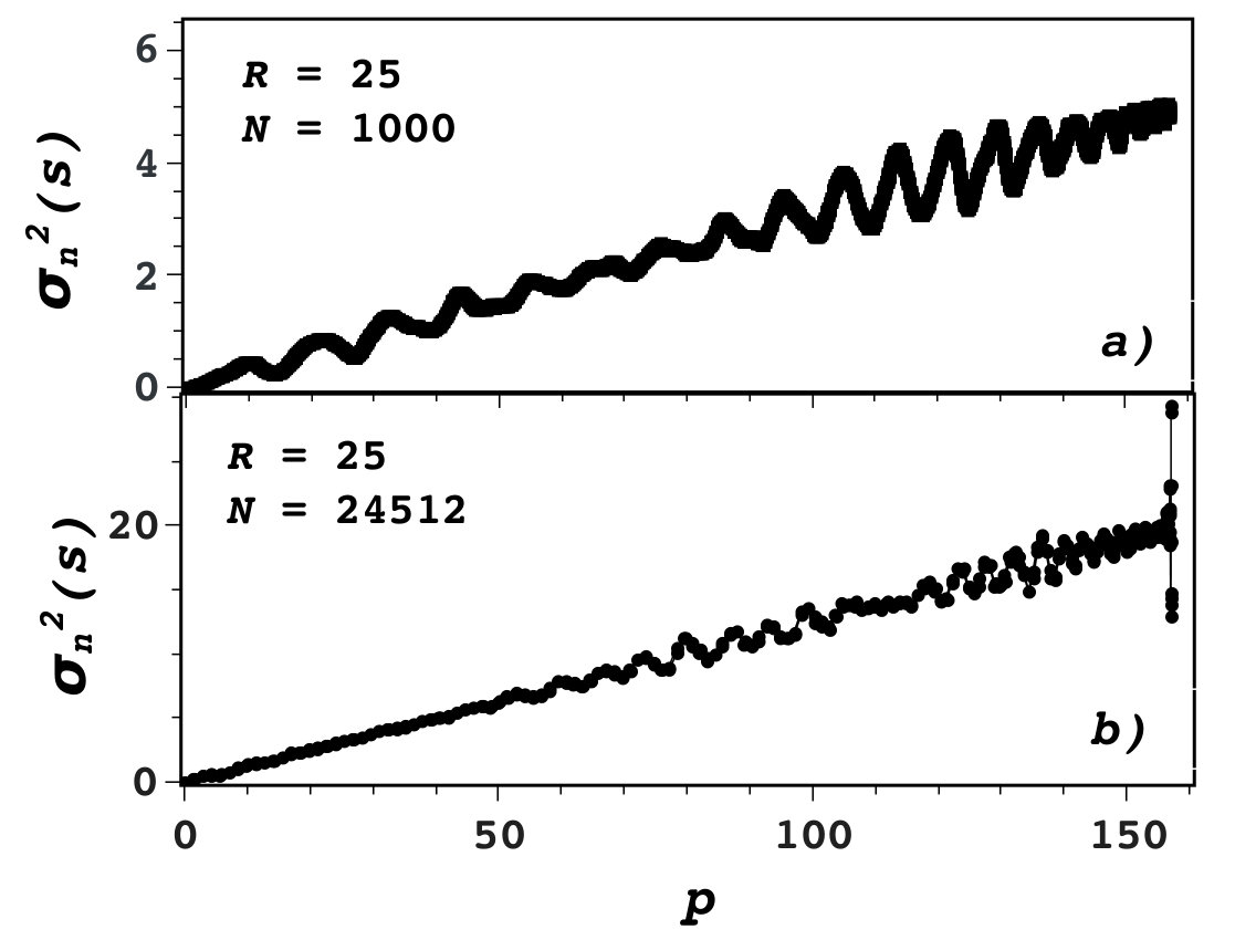 Figure 3
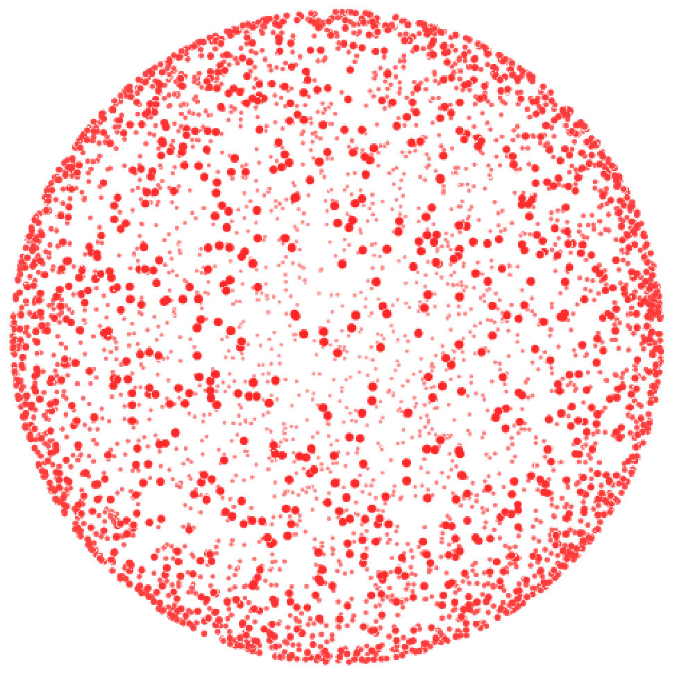 Figure 4
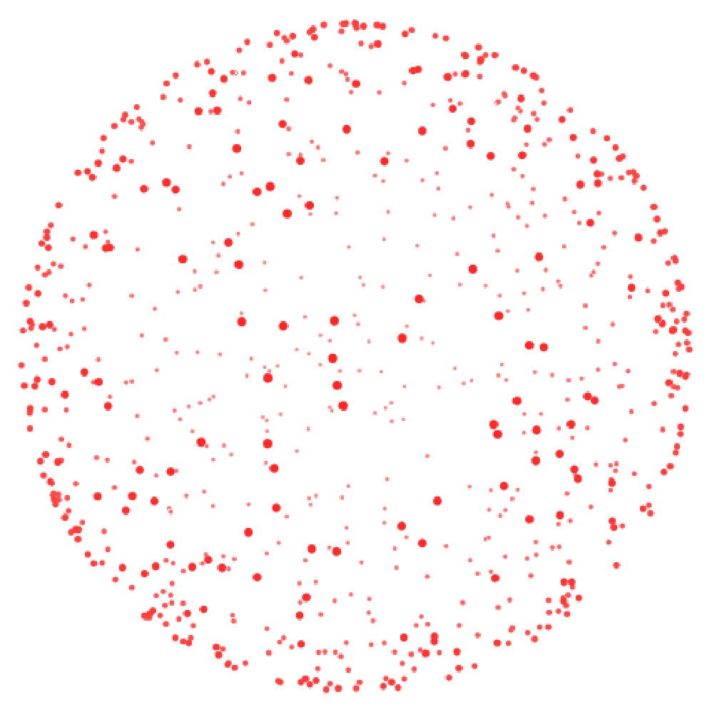 Figure 4
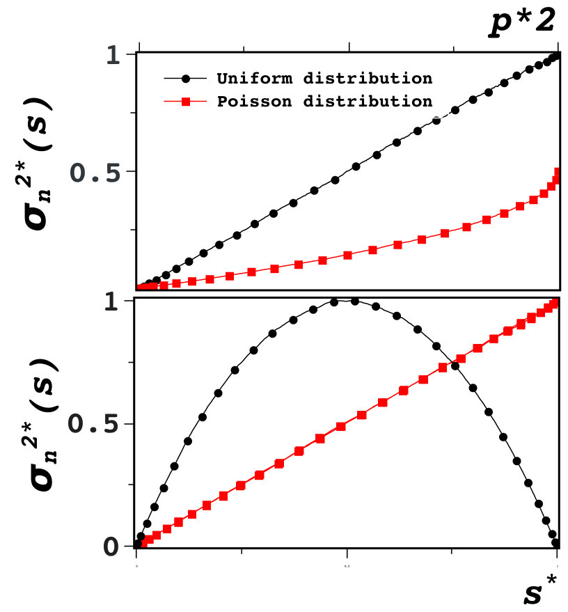 Figure 5
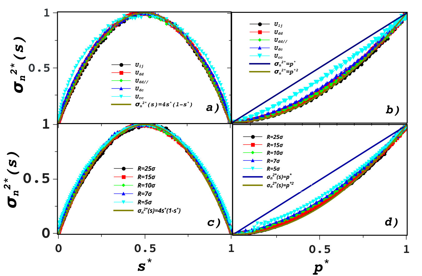 Figure 6
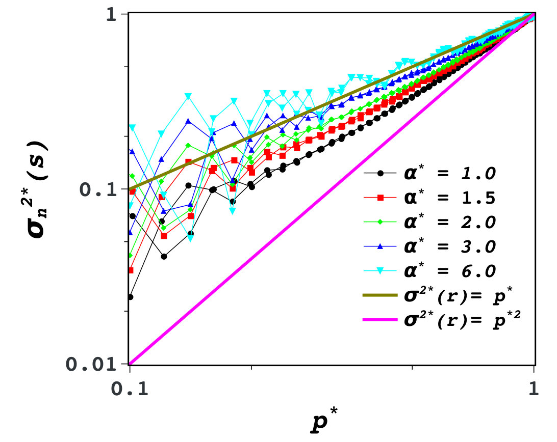 Figure 8
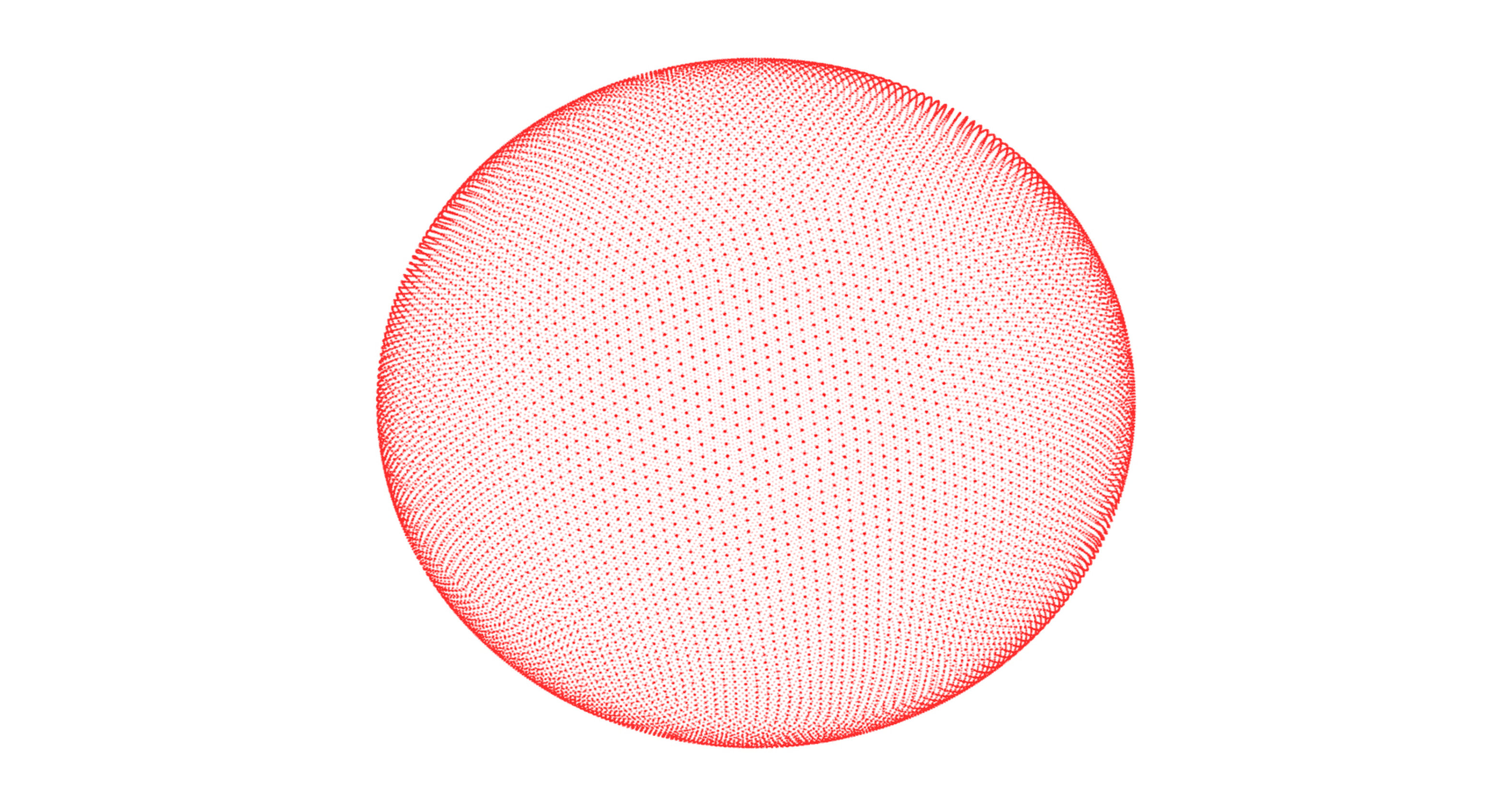 Figure 13
| Point pattern | scaling |
|---|---|
| Poisson distribution | |
| Uniform distribution | |
| Triangular lattice | |
| Fibonacci lattice |
Peer Reviews
No public reviews on file for this paper yet. If you reviewed it on a platform where reviews are public (OpenReview, ICLR, NeurIPS, ICML), you can paste yours below so the community can read it here.
Videos
No videos yet. Explain this paper in a talk, walkthrough, or lecture? Add one.
Hyperuniformity on spherical surfaces
Ariel G. Meyra1,2, Guillermo J. Zarragoicoechea1,3, Alberto. L. Maltz4, Enrique Lomba2, and Salvatore Torquato5,6
1IFLYSIB (UNLP, CONICET), 59 No. 789, B1900BTE La Plata, Argentina
2Instituto de Química Física Rocasolano, CSIC, Calle Serrano 119, E-28006 Madrid, Spain
3Comisión de Investigaciones Científicas de la Provincia de Buenos Aires, Argentina
4Departamento de Matemática, Facultad de Ciencias Exactas, Universidad Nacional de La Plata, CC 72 Correo Central 1900 La Plata, Argentina
5Department of Chemistry, Princeton University, Princeton, New Jersey 08544, USA,
6Princeton Institute for the Science and Technology of Materials, Princeton University, Princeton, New Jersey 08544, USA
Abstract
In this work we present a study on the characterization of ordered and disordered hyperuniform point distributions on spherical surfaces. In spite of the extensive literature on disordered hyperuniform systems in Euclidean geometries, to date few works have dealt with the problem of hyperuniformity in curved spaces. As a matter of fact, some systems that display disordered hyperuniformity, like the space distribution of photoreceptors in avian retina, actually occur on curved surfaces. Here we will focus on the local particle number variance and its dependence on the size of the sampling window (which we take to be a spherical cap) for regular and uniform point distributions, as well as for equilibrium configurations of fluid particles interacting through Lennard-Jones, dipole-dipole and charge-charge potentials. We will show how the scaling of the local number variance enables the characterization of hyperuniform point patterns also on spherical surfaces.
I Introduction
Since the pioneering work of Torquato and Stillinger in the early 2000s Torquato and Stillinger (2003), hyperuniformity has been the focus of a large collection of works of relevance in the fields of physics (e.g. random jammed hard-particle packings Donev et al. (2005), driven nonequilibrium granular and colloidal systems and sand pile models Hexner and Levine (2015); Weijs et al. (2015); Tjhung and Berthier (2015); Dickman and da Cunha (2015), and dynamical processes in ultracold atoms Lesanovsky and Garrahan (2014)), materials science (photonic band-gap materials Florescu et al. (2009); Man et al. (2013); Froufe-Pérez et al. (2017), dense disordered transparent dispersions Leseur et al. (2016), composites with desirable transport, dielectric and fracture properties Zhang et al. (2016); Chen and Torquato (2018); Xu et al. (2017); Wu et al. (2017), polymer-grafted nanoparticle systems Chremos and Douglas (2017), and “perfect” glasses Zhang et al. (2017)), and biological systems (photoreceptor mosaics in avian retina Jiao et al. (2014), and immune system receptors Mayer et al. (2015)). The defining characteristic of these hyperuniform systems is the anomalous suppression of density (particle number or volume) variances at long wavelengths. In Euclidean space this implies that the structure factor tends to zero as the wavenumber Torquato and Stillinger (2003), i.e.,
[TABLE]
Here is the Fourier transform of the total correlation function , is the pair correlation function and is the number density.
Hyperuniformity in most of the systems enumerated above is a large scale structural property defined in an Euclidean space. However, strictly speaking, one can also transfer the concept to non-Euclidean geometries. A particular case of relevance in this connection is the avian photoreceptor distribution, which, if one is to consider it rigorously, must be treated on a curved surface, that of the retina. Obviously, to a first approximation, if the size of the receptors is small compared to the intrinsic curvature of the retina, one can reduce the problem to that of a particle distribution on a flat surface. However, this does not have to be necessarily the case in all instances. The extension of the concept of hyperuniformity to sequences of finite point sets on the sphere was introduced in the very recent works of Brauchart and coworkers Brauchart et al. (2018, ), where the problem is addressed from a formal mathematical perspective and connected to the more general problem of spherical designs. Point pattern designs on spherical surfaces are key in the development of optimal Quasi Monte Carlo (QMC) integration schemes Brauchart et al. (2014). These have been extensively used to construct efficient quadratures to evaluate illumination integrals which are essential in the rendering of photorealistic images Marques et al. (2015). Brauchart and coworkers Brauchart et al. (2018) have shown that these optimal QMC design sequences are hyperuniform. In Ref. Brauchart et al. (2014) it was shown that good candidates to build QMC spherical designs could be devised from sets of points minimizing Coulomb or logarithmic (i.e. two-dimensional Coulomb) pairwise interactions. We will see here how this finding is reflected by our own results.
On the other hand, from a materials science perspective, the realization of particle designs on curved surfaces at the microscopic level, has been experimentally achieved by means of self-assembly of colloidal particles on oil/glycerol interfacesIrvine et al. (2012). This opens an avenue to experimentally devise and manipulate hyperuniform systems on curved surfaces at will. Bearing in mind the relevance of hyperuniformity for the accurate representation of images (both in bird retina and in artificial image rendering), the potential technological implications of these experimental achievements are obvious.
In order to further our understanding of hyperuniform systems in curved spaces, in this paper we have addressed the characterization of the local particle number variances on a collection of point and particle distributions on spherical surfaces. Given the finite size of our systems, the use of the infinite wavelength criterion of the structure factor to elucidate the presence of hyperuniformity is inadequate. This means that the structural characterization of hyperuniform designs on the sphere must be focused on the density/number variances. Obviously, in the limit of infinite sphere radius with number density fixed, the properties of the system will approximate those of the Euclidean case, and Eq. (1) will be again useful as a signature of hyperuniformity. This large size connection between curved and Euclidean geometries was already exploited by Caillol et al. Caillol et al. (1981) to remove the effects of periodic boundary conditions in molecular simulations, and cope with the long range of Coulombic interactions without resorting to the use of Ewald summations or similar techniques.
In practice, here we will analyze the scaling of the local particle number variance defined as
[TABLE]
where denotes the area of sampling spherical cap, and is the number of particles contained in the sampling window, as in Ref. Brauchart et al. (2018) (see Figure 1). The bar in (2) denotes an statistical average within the sampling window over the spherical surface. In practice, in this work we will be dealing with point distributions composed of finite sets of N points placed on the surface of a sphere of radius and total area . From the work of Brauchart et al.Brauchart et al. (2018) on hyperuniform point sets on the sphere, we know that for the uniform Poisson distribution the local number variance scales with the surface of the sampling window, i.e. . In contrast, in hyperuniform systems . In Section II we will introduce explicit expressions connecting the number variance with structural properties, such as the pair distribution function.
In order to properly describe hyperuniformity on the curved sphere, in Section III we have first analyzed the behavior of the number variance of regular point patterns on the spherical surface, namely a triangular grid and a Fibonacci lattice. Since spatially ordered point patterns such as those of crystals in Euclidean space (or partly ordered, such as quasicrystals) are known to be hyperuniform, one should clearly expect the same to happen on the spherical surface. Next, on the opposite end, we have checked the behavior of Poisson patterns and uniform distributions. It is important to remark that Poisson patterns on the sphere cannot be built with a fixed particle number, N. For a given average surface density one generates a series of point realizations, , with a total number of points, , whose average is according to a Poisson distribution (see Appendix). This implies that we will be studying two different types of ensembles, one characterized by constant (canonical-like), and another characterized by a constant and variable (grand canonical-like).
In this way we will have a set of reference systems defining ordered hyperuniform and disordered non-hyperuniform structures. We have then studied the behavior of fluid particles confined on the spherical surface and interacting via potentials with different ranges, from short range Lennard-Jones interactions, to dipolar like (i.e. ) and 3D Coulomb (plasma-like) (i.e. ) interactions. To that aim we have run canonical Monte Carlo simulations for various sphere sizes and a fixed surface density. We will see the correspondence between the hyperuniform and the non-hyperuniform reference systems on the spherical surface and in Euclidean space, and then we will see how the interactions and the size of the sphere play a role in the build up of disordered hyperuniform states on this non-Euclidean space. The article is closed with a brief summary and future prospects.
II Explicit Formulas for the Number Variance on a Sphere
Consider a single configuration of points on the 2-sphere , i.e., surface of a three-dimensional sphere of radius , as depicted in Figure 1. It is assumed that both and are large and of comparable magnitude to one another. Let and denote the base radius and the height of a spherical cap, respectively. The surface area of a spherical cap is where we will be considering only the upper hemisphere, to avoid ambiguity. The number density of the points on the sphere is given by , and is the number of points contained within a spherical-cap window centered at position on the sphere. Let the window uniformly sample the space for sufficiently small , i.e., is much smaller than . Following Torquato and Stillinger Torquato and Stillinger (2003) for the formulation in Euclidean space, the number variance associated with a single configuration on the sphere is given by
[TABLE]
where denotes again an average of a random variable over and is the intersection area of two spherical caps whose centers are separated by a geodesic distance , divided by the area of a cap. Because the variance formula (3) is valid for a single realization, one can use it to find the particular point pattern that minimizes the variance at a fixed value of , i.e., one can find the ground state for the “potential energy” function represented by the pairwise sum in (3).
Now imagine that we generate many realizations of a large particle number on the surface of the sphere so that the density is fixed and then consider the thermodynamic limit. The ensemble-averaged number variance, , follows immediately from (3). We find
[TABLE]
where is the geodesic pair correlation. Brauchart et al. Brauchart et al. (2014) rigorously studied the behavior of the number variance in the large- limit. For any “uncorrelated” point process, for , we have
[TABLE]
where we have used the identity . We call a point process on hyperuniform if, as becomes large,
[TABLE]
In our particular case, from Brauchart et al. Brauchart et al. , the normalized intersection area is given by
[TABLE]
and zero otherwise, where is the angle between the vectors pointing to the center of the two intersecting spherical caps. It can be shown that in the limit of , Eqs. (4) and (7) reduce to the expressions found in Ref. Torquato and Stillinger (2003) for the Euclidean case in two dimensions.
III Number variance of regular point patterns on a spherical surface
In this and the subsequent sections, we perform our analysis of the local particle number variance defined in Eq.(2) using a spherical cap as illustrated in Figure (1). In order to perform an adequate sampling of the number variance, a sufficiently large number of centers of the sampling spherical cap must be chosen randomly on the surface (around 10000). In the case of fluid particles, only three centers (in orthogonal directions) are chosen and then averages are performed over configurations. Now, since we also analyze the dependence of the results on the total area of the system, or equivalently, the number of particles, it will be convenient to define normalized quantities, such as the normalized arc length of the spherical cap, , the normalized area of the sampling region, , and the normalized perimeter, . Note that these two quantities are related by . Also, the number variance will be normalized as = , where the subscript indicates the maximum value of the variance. This will facilitate the presentation of the results and analysis of the scaling relations.
Now, we will first consider the number variance associated with regular point patterns (in Euclidean spaces crystals are the most familiar regular spatial point patterns). Building a two dimensional lattice on an spherical surface is a non trivial problem, and it is certainly very useful in the field of astronomical observation. Here we will resort to the icosahedron method proposed by Tegmark Tegmark (1996) as an alternative for pixelizing the celestial sphere. We refer the reader to Tegmark (1996) for the details of the algorithm. The resulting point distribution is illustrated on the upper left graph of Figure 2. Note that this is an approximate triangular grid since the algorithm maps the triangular faces of an icosahedron in which the sphere is inscribed onto the surface of the sphere, and then distorts the points to give all pixels approximately the same area. Another alternative that yields equal area for all grid points are the Fibonacci grids. Swinbank and Purser have proposed an efficient algorithm to produce this very regular grid on a spherical surface Swinbank and Purser (2006). Again, we refer the reader to the original reference for a detailed description of the algorithm. The corresponding illustration of the Fibonacci pattern can be seen in the lower left graph of Figure 2. These procedures devised to obtain pixels of approximately the same area on the sphere surface, are similar in spirit to the Quasi Monte Carlo approach for numerical integration on spherical surfaces discussed by Brauchart et al.Brauchart et al. (2018). In the latter instance, one must choose a set of points that minimizes the error of numerical integration, and this in turn leads to pixels of similar size on the sphere’s surface. In Ref. Brauchart et al. (2018) it was shown that this corresponds to a hyperuniform point distribution. The minimization constraint makes the approach deterministic, retaining nonetheless some Monte Carlo (i.e. stochastic) character. In contrast, the result of our two tessellation techniques would be the spherical geometry equivalent of regular grid integration sets in Euclidean spaces.
The of the two regular point patterns is presented in the right graph of Figure 2. One observes in both cases the presence of oscillations resulting from the almost ordered structure of our systems. On the other hand in both instances the analysis clearly shows that we have a scaling of the number variance linear with the perimeter, . This will correspond to the linear dependence on the radius of the sampling window in perfectly ordered lattices in a flat two dimensional space, in which the perimeter of the sampling window is proportional to its radius. This latter relation does not hold on the spherical surface. In our study we have found that no simple scaling can be derived using the arc length, , or the area, , of the sampling spherical cap. This is a necessary consequence of the finite character of our sampling space, since when then , which implies a non monotonous dependence on the sampling area. In contrast, presents a monotonous dependence on .
IV Variances of a random uniform and Poisson spatial
distributions of points
On the other end we have “uniformly” disordered systems, such as the random uniform point distribution and the Poisson point distribution on a sphere.
First, we focus on the local number variance of point patterns following a random uniform distribution. The generation of this point configuration is a trivial problem in Euclidean spaces using pseudo-random numbers. Here, one must be a bit more careful. The simplest approach is to generate a uniform distribution of points inside a cube inscribing the sphere, discarding those points outside the sphere, and then performing an orthogonal projection of the inner points onto the surface. Alternatively one can choose three pseudo-random numbers following a Gaussian distribution centered in the sphere of radius, , and project the resulting point in space onto the spherical surface. Other approaches can also be found in Ref. Weisstein (2018). has been analyzed for different sphere radii and number densities and the results, once normalized as indicated in Section III collapse onto a single curve, which follows the known exact result, , as can be seen in Figure 3.
On the other hand, the generation of a Poisson point distribution on a spherical surface is not straightforward. Here it has been generated by an algorithm devised following the considerations of BaddeleyBaddeley (2004). For completeness a detailed description of the algorithm is included in the Appendix. A characteristic Poisson configuration on the spherical surface is illustrated in Figure 3. Note again that the configurations so generated will be characterized by an average surface density, , and in contrast with the previously discussed uniform distribution, we will not have a system with a fixed number of points, . Instead we will have a collection of systems whose average yields the average density, . As mentioned before, to some extent, this formulation recalls the relation between grand canonical and canonical ensembles. In contrast with the uniform distribution, the maximum of the Poisson distribution variance for a given is now reached when .
In Figure 3c we present the scaling of the normalized number variance vs the normalized area for Poisson patterns. One observes, a complete linear dependence and the absence of oscillations characteristic of a spatially disordered and to some extent uniform distribution. This dependence is fully consistent with that of Poisson patterns on flat surfaces, Torquato and Stillinger (2003). Interestingly, if we now try to look for the same scaling for the the strictly uniform (constant surface density) point distribution, one finds that it does not conform to the surface scaling relation. In consonance with our findings for ordered, regular patterns, we see in Figure 3c that . Thus, it turns out that the perimeter will now again be the scaling variable. In analogy with the definitions for Euclidean spaces, we will consider systems with fixed N and squared perimeter variance scaling as non-hyperuniform.
In this way, we have defined what will be our reference results for scaling of the local number variance on the spherical surface. We will see that intermediate situations between linear and quadratic scaling will also be possible, following
[TABLE]
that from Eq.(6) will also correspond to hyperuniform configurations. A summary of the systems considered up to this point is presented in Table 1.
V Number variances in fluids of interacting particles
In this section, we present some results of Monte Carlo simulations in a canonical ensemble (particle number, area and temperature fixed) for particles on a spherical surface interacting with the potential functions summarized below in Eqs. (9) and (10). In what follows, , and are the number of molecules, the sphere area, and temperature, respectively. The simulation starts when N particles are randomly placed on a sphere surface of radius . We then perform translational attempts along random directions on the surface in order to equilibrate the system. Averages are calculated over statistically independent configurations. Here we will analyze the effect of different interactions and sphere radii (system size) on the local particle number variances. Bearing in mind the results of the previous Section, we will be able to see how the interaction tunes the hyperuniform character of the fluid structure.
The net interparticle interaction has a short range dispersive/repulsive component of the Lennard-Jones (LJ) form:
[TABLE]
where the Lennard Jones parameters, and , are taken as the energy and length scale respectively. A reduced temperature is defined and set to , well above the critical temperature for a LJ fluid practically confined in a two dimensional space. Distances will be scaled as , and , and density as . It must be stressed that is the Euclidean distance between particles and , and not the arc length. Our particles are actually three dimensional entities with three dimensional interactions restricted to move on the sphere’s surface. To the LJ interaction we will add dipolar-like, charge-dipole, and charge-charge contributions. To simplify the problem, dipoles are kept perpendicular to the surface, as if under the influence of an electric field whose source is at the center of the sphere. We will also consider the case of purely parallel dipoles, which leads to a simple repulsion, and for the charge-dipole interaction we will also consider that dipoles are orthogonal to the line joining the particle centers. This is a crude approximation to the case of dipoles perpendicular to the surface. The explicit form of the interactions used is:
[TABLE]
where = 1 and will be set to unity in most cases, except when analyzing the effect of the repulsion strength on the number variance and pattern formation.
We have determined the local number variance for two different radii, and . This is plotted for the latter case in Figure 4 using normalized quantities. Results for are omitted since they are qualitatively very similar. In the right graph of Figure 4 two reference curves have been added, one representing the linear dependence on the sampling area perimeter (strongly hyperuniform scaling) and another for the quadratic dependence (regular disordered non-hyperuniform systems). One immediately observes that as the range of the potential increases, the scaling becomes hyperuniform, i.e. with , and decreasing as the interaction range increases. In fact, for the Coulomb like interaction we have Note the this interaction gives strictly for planar surfacesLomba et al. (2018). The pure LJ fluid, as in the Euclidean case, displays no hyperuniformity, and conforms to the same scaling as the uniform random point patterns.
Interestingly, a comparison of the pair distribution functions, , for different interactions (not shown), tuning just the long range component as we have done in the results of Figure 4, does not show the emergence of any particular feature when hyperuniformity builds. As shown in Ref. Lomba et al. (2017), hyperuniformity seems to be associated with the build up of some sort of long range order involving more than two particles, which is not easily captured by pairwise quantities such as , except in the infinite long range limit (, ), which is not accessible in the present instance.
Now, in the lower graphs of Figure 4 we observe how the size of the “confining” sphere affects the local particle number variance. To that aim we have just focused on the dipolar-like interaction. The repulsion leads to a hyperuniform behavior in three dimensions, and quasi-hyperuniformity in two dimensions (see Eq. (4) in Ref. Lomba et al. (2018)). We see that for large spheres (), practically scales as a uniform random point distributions, and it finally deviates somewhat for the smallest sphere. This is an indication that curvature (whose relative effect is increased as the size is smaller with fixed surface density) seems to enhance hyperuniform-like behavior.
We turn now to the analysis of the interaction strength effects. To that purpose we choose the dipole-dipole potential, in Eq.(10), and vary the interaction strength parameter, , from 1 to 6. The effect on the local number variance is visible in Figure 5. One can clearly observe that as the strength of the interaction increases (and consequently its effect on the long range order is enhanced) the degree of hyperuniformity grows, until finally for we are back to the linear scaling (strong hyperuniformity) with the characteristic oscillations of an almost ordered regular pattern. This pattern formation is readily seen in the snapshots of Figure 6. One appreciates there that for the largest interaction strength the particles are almost ordered in a trigonal lattice. This is mostly an energetic effect (even if entropy is also maximized), by which the particles adopt a configuration that maximizes the interparticle distances, thus minimizing the repulsive energy. With this quasi-ordered state we are back to the purely linear dependence of the local number variance of the trigonal and Fibonacci lattices. This low temperature (or high ) states recall the point patterns that minimize the Coulomb energy, which according to Ref. Brauchart et al. (2014) provide suitable spherical designs for QMC integration.
All other intermediate disordered situations are also hyperuniform, but interestingly none of them (and neither does the pure Coulomb repulsion) reaches at finite non-zero temperature the limiting behavior of ordered structures, . This is in contrast with the situation found for plasmas in Euclidean space Lomba et al. (2017, 2018) which produce structural hyperuniform configurations at any finite temperature.
Finally, we see now how the structuring of the fluid as a consequence of the increasing interaction strength reflects on the pair distribution function depicted in Figure 7. Here the build up of strong short range order is seen in the marked oscillations of for . The fact that one obtains a smooth curve and not the sharp spikes typical of solids is the result of the thermal motion of the particles around the equilibrium positions and the curved nature of the sampling space.
VI Conclusion
In summary, we have shown that, in parallel with the situation found in Euclidean space, point configurations on a sphere surface may exhibit two types of scaling of the local number variance with the size of the sampling window: regular point patterns display a linear dependence on the perimeter of the sampling window, and uniform point patterns show a quadratic dependence. Strict Poisson distributions (characterized by an average density) have local number variances that depend linearly on the area of the sampling window. Due to the curvature of the space, the area of sampling window does not depend quadratically on the perimeter, in contrast with the flat two dimensional situation. Additionally, we have seen how increasing the long range of the interaction enhances the degree of the hyperuniformity. A similar effect is found when decreasing the size of the sphere where the sample is contained. This can be understood in terms of the increase of the relative interaction range in terms of system size. Finally, we see that for the dipolar interaction (and most likely for all repulsive interactions of medium/long range), increasing the strength of the interaction also induces a higher degree of hyperuniformity, finally leading to the formation of regular ordered patterns.
Future work will focus on the study of different geometries, such as cylinders or ellipsoids, of relevance in technology and biological systems. We also plan to study the effect of interactions that favor the formation of quasi-crystal structures, in particular those that implement highly directional bonding interactions as found in patchy colloids.
Acknowledgements.
The authors are grateful to Jaeuk Kim for his careful reading of the manuscript. AGM, GZ and EL acknowledge the support from the European Union’s Horizon 2020 Research and Innovation Programme under the Marie Skłodowska-Curie grant agreement No 734276. EL also acknowledges funding from the Agencia Estatal de Investigación and Fondo Europeo de Desarrollo Regional (FEDER) under grant No. FIS2017-89361-C3-2-P. S. T. was supported in part by the National Science Foundation under Award No. DMR-1714722.
Appendix A Generating a Poisson point distribution on a sphere.
We recall that a random variable whose values are the non-negative integers has a Poisson distribution with parameter whenever for . It is often abbreviated by saying that has a distribution. Some basic properties are:
- •
If has a distribution then
- •
If are independent random variables having distributions respectively, then has a distribution.
Let be a sphere. For each region we denote its area by . Suppose that we have a random distribution of points on the sphere. For each region we denote the random variable “number of points in .” We have a random spatial point process with parameter whenever
- •
For each , has a distribution.
- •
If are mutually disjoint regions then are independent random variables.
We recall that each point in the sphere has two angular spherical coordinates and . In order to generate a set of points distributed according to a Poisson spatial process on the sphere with parameter we have developed an algorithm based in an usual idea in this subject:
We subdivide the sphere into small, mutually disjoint “spherical rectangles” so that the angular coordinates of every point in satisfy inequalities of the form and . 2. 2.
For each we generate a random number according to a distribution and points uniformly distributed in are generated.
The reference list from the paper itself. Each links out to its DOI / PubMed record.
- 1Torquato and Stillinger (2003) S. Torquato and F. H. Stillinger, Phys. Rev. E 68 , 041113 (2003) . · doi ↗
- 2Donev et al. (2005) A. Donev, F. H. Stillinger, and S. Torquato, Phys. Rev. Lett. 95 , 090604 (2005).
- 3Hexner and Levine (2015) D. Hexner and D. Levine, Phys. Rev. Lett. 114 , 110602 (2015).
- 4Weijs et al. (2015) J. H. Weijs, R. Jeanneret, R. Dreyfus, and D. Bartolo, Phys. Rev. Lett. 115 , 108301 (2015).
- 5Tjhung and Berthier (2015) E. Tjhung and L. Berthier, Phys. Rev. Lett. 114 , 148301 (2015).
- 6Dickman and da Cunha (2015) R. Dickman and S. D. da Cunha, Physical Review E 92 (2015), 10.1103/physreve.92.020104 . · doi ↗
- 7Lesanovsky and Garrahan (2014) I. Lesanovsky and J. P. Garrahan, Phys. Rev. A 90 , 011603 (2014).
- 8Florescu et al. (2009) M. Florescu, S. Torquato, and P. J. Steinhardt, Proc. Nat. Acad. Sci. 106 , 20658 (2009).