Wavefield Finite Time Focusing with Reduced Spatial Exposure
Giovanni Angelo Meles, Joost van der Neut, Koen W. A. van Dongen, Kees Wapenaar

TL;DR
This paper introduces a new double-sided wavefield focusing method that reduces spatial exposure and finite-time signals, improving focus quality in heterogeneous media like brain imaging.
Contribution
It presents an alternative integral representation for double-sided wavefield focusing with finite in- and output signals, reducing wave propagation through the medium.
Findings
Finite-time input signals are sufficient for focusing.
Wave energy propagation is reduced compared to traditional methods.
Numerical experiments demonstrate improved focusing in a head model.
Abstract
Wavefield focusing is often achieved by Time-Reversal Mirrors, where wavefields emitted by a source located at the focal point are evaluated at a closed boundary and sent back, after Time-Reversal, into the medium from that boundary. Mathematically, Time-Reversal Mirrors are derived from closed-boundary integral representations of reciprocity theorems. In heterogeneous media, Time-Reversal Focusing theoretically involves in- and output signals that are infinite in time and the resulting waves propagate through the entire medium. Recently, integral representations have been derived for single-sided wavefield focusing. Although the required input signals for this approach are finite in time, the output signals are not and, similar to Time-Reversal Mirroring, the resulting waves propagate through the entire medium. Here, an alternative solution for double-sided wavefield focusing is…
Click any figure to enlarge with its caption.
 Figure 1
 Figure 2
 Figure 3
 Figure 4
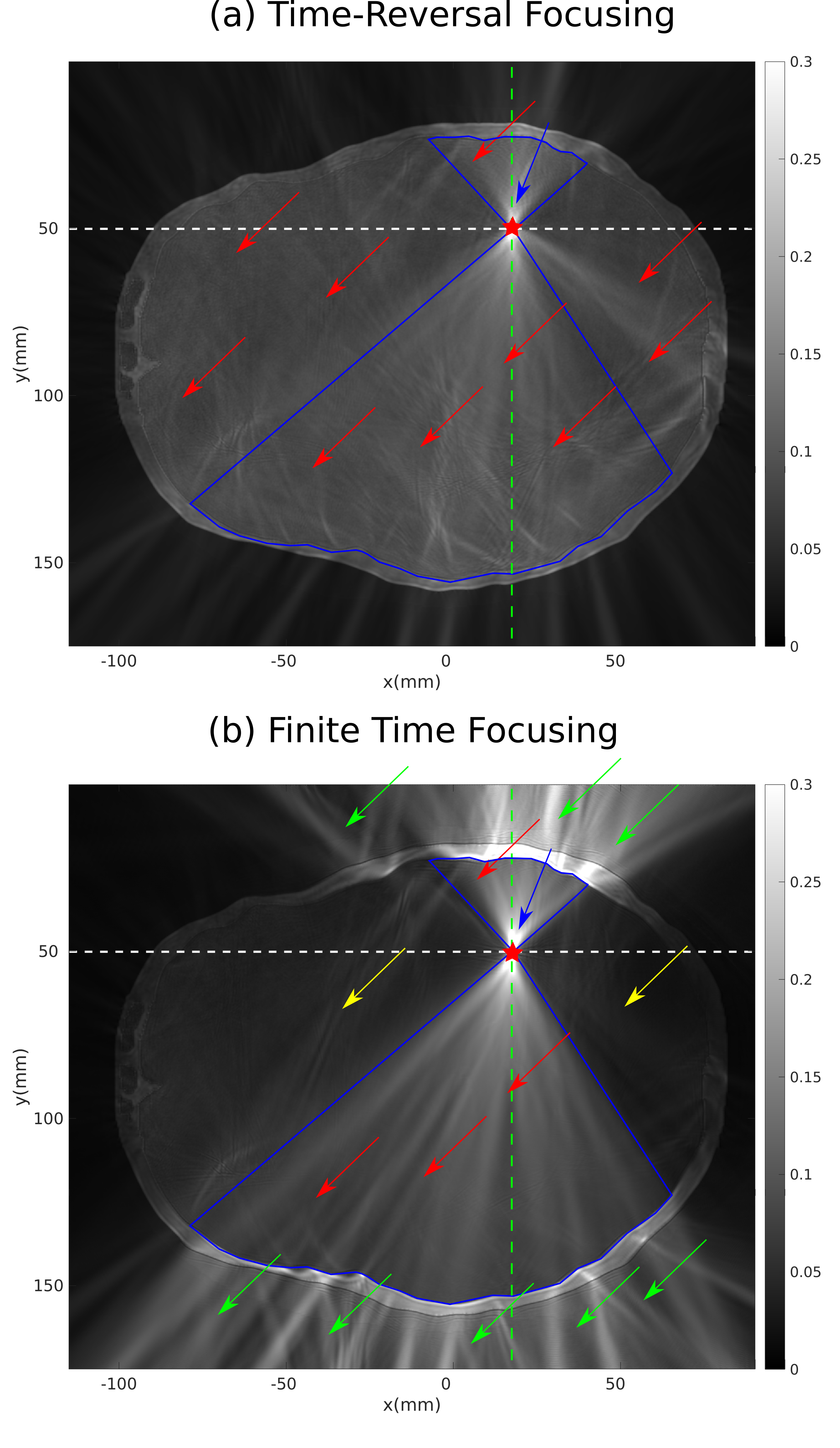 Figure 5
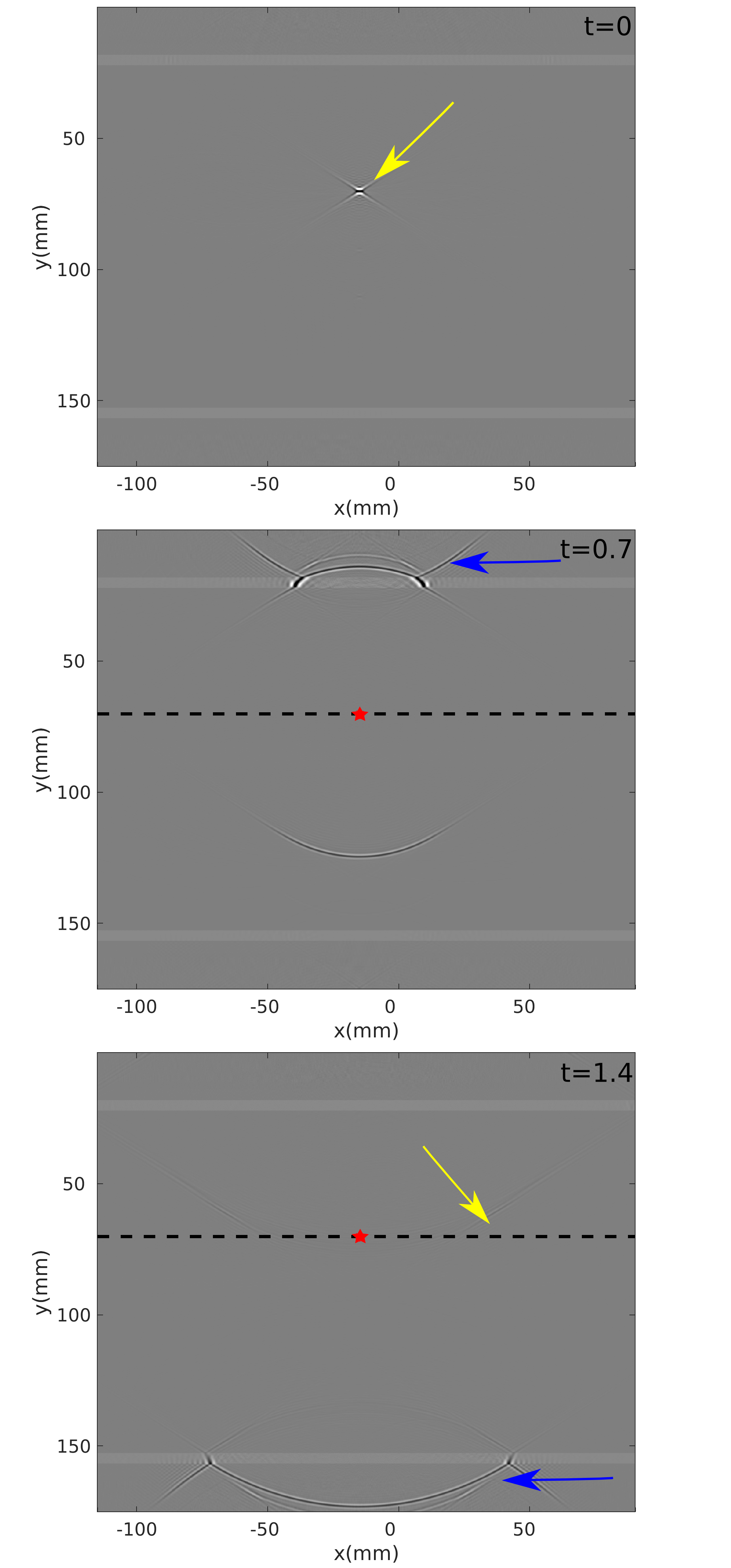 Figure 6
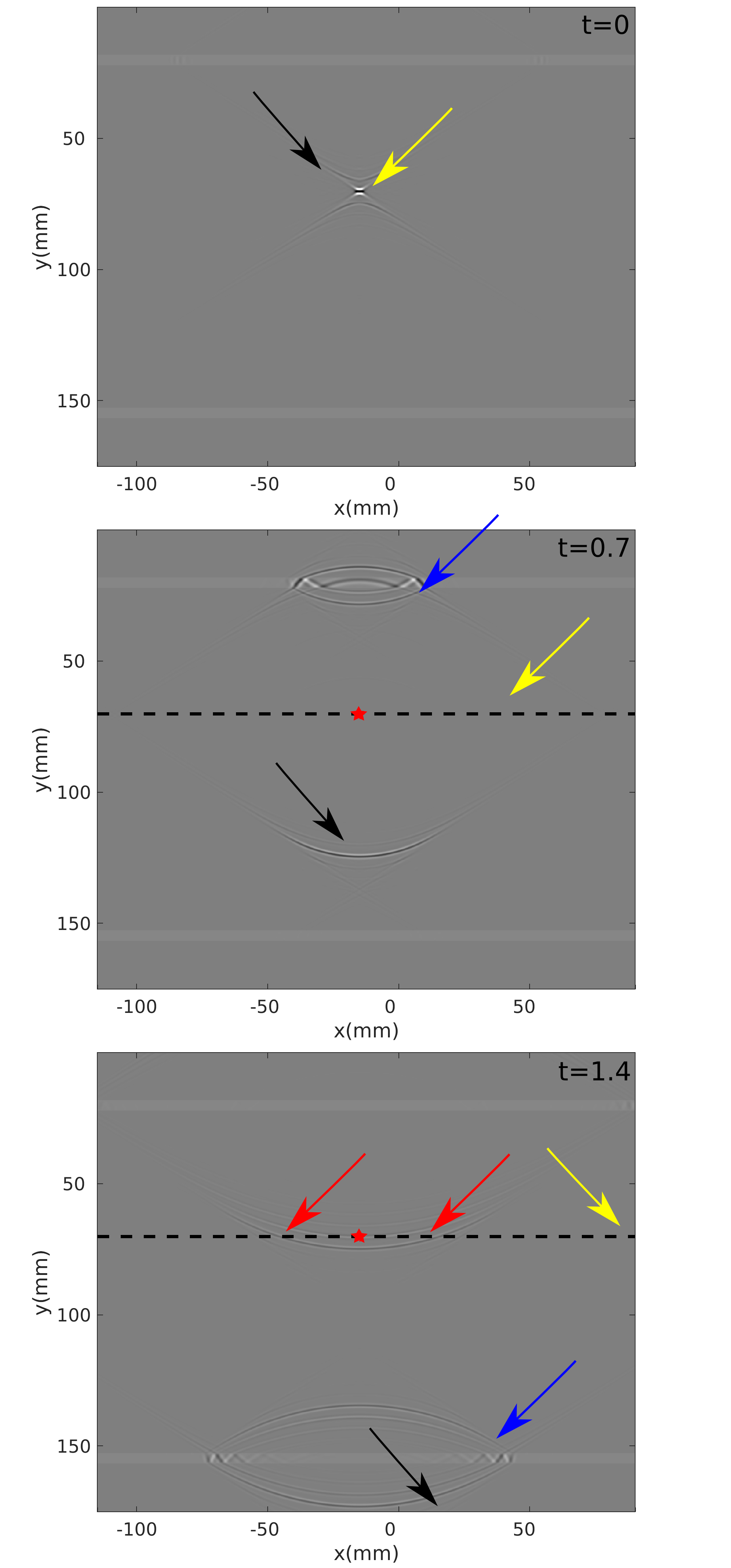 Figure 7
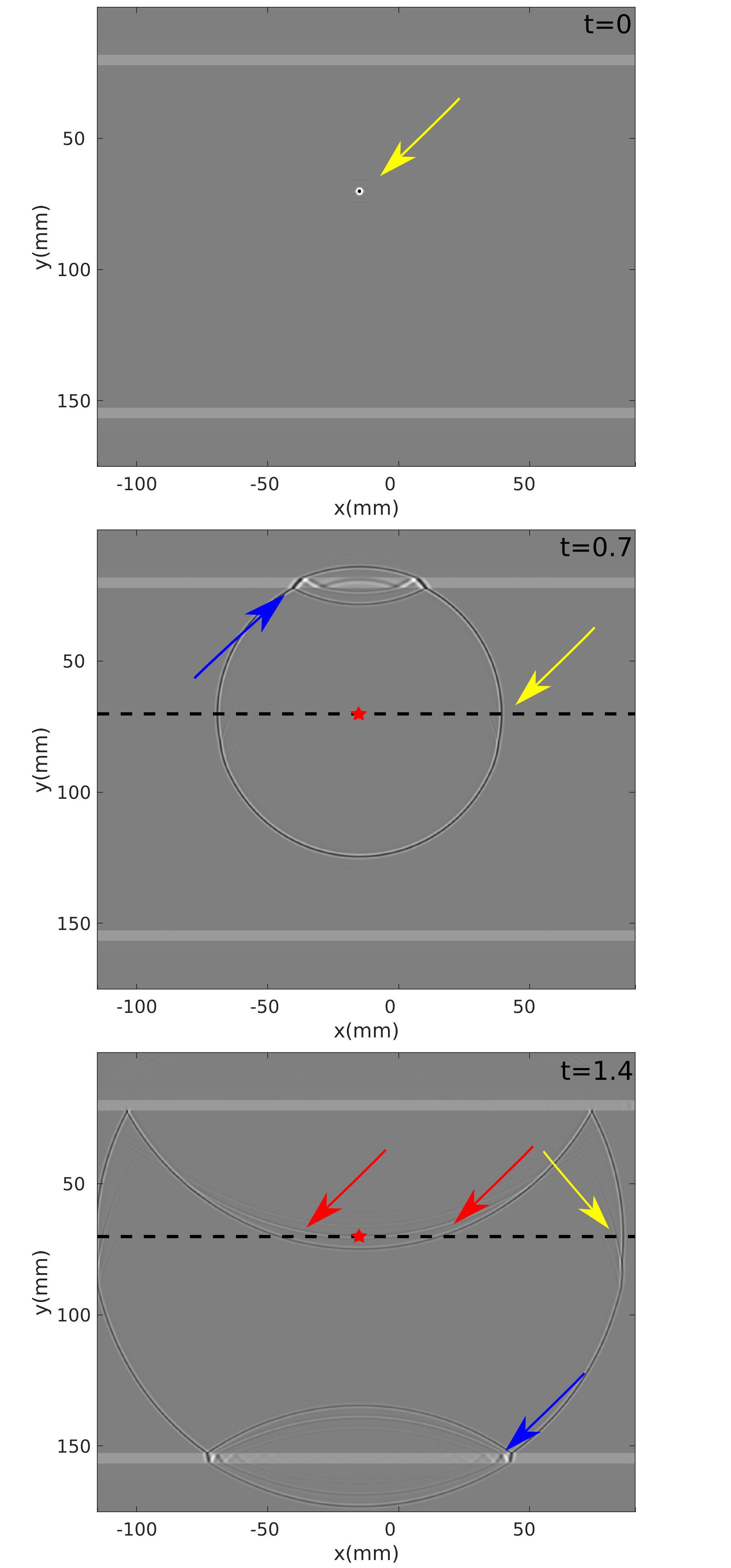 Figure 8
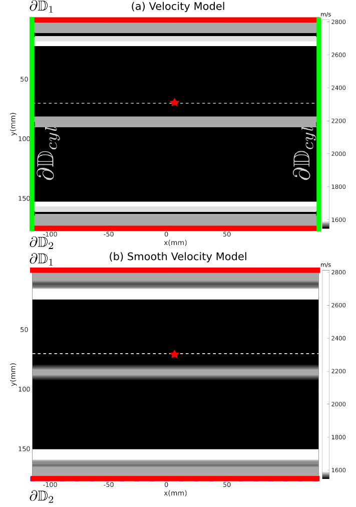 Figure 9
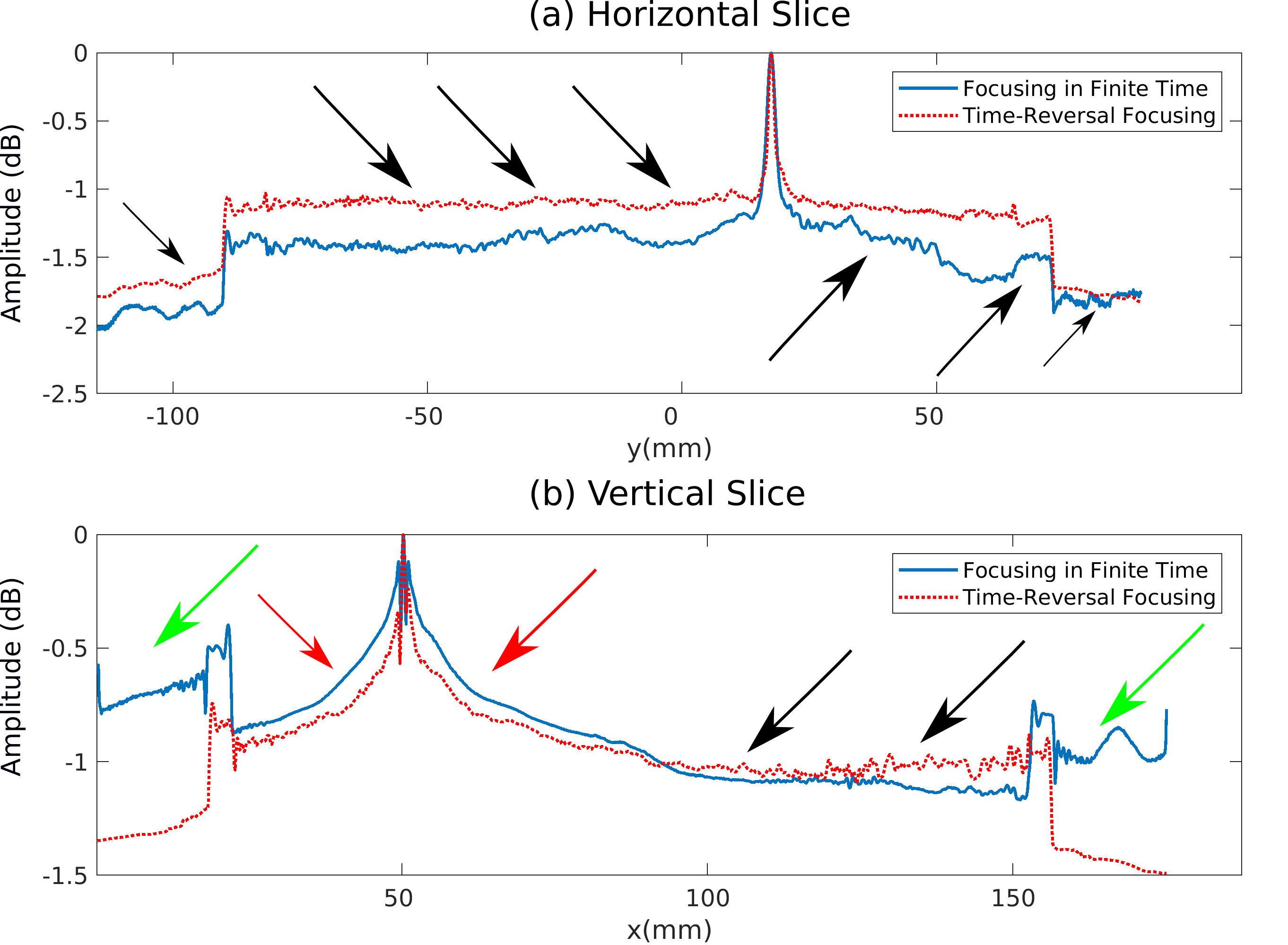 Figure 10
| Tissue | velocity (m/s) | density (kg/m3) |
|---|---|---|
| Muscle | 1588 | 1090 |
| Skull | 2813 | 1908 |
| Water | 1578 | 994 |
| Blood | 1578 | 1050 |
| Brain | 1546 | 1046 |
| Brain | Blue Cones | Red Cones | |
|---|---|---|---|
| SMF | +1% | +16% | -26% |
| FTF | -14% | +5% | -45% |
Peer Reviews
No public reviews on file for this paper yet. If you reviewed it on a platform where reviews are public (OpenReview, ICLR, NeurIPS, ICML), you can paste yours below so the community can read it here.
Videos
No videos yet. Explain this paper in a talk, walkthrough, or lecture? Add one.
Wavefield Finite Time Focusing with Reduced Spatial Exposure
Giovanni Angelo Meles
Faculty of Civil Engineering and Geosciences
Delft University of Technology
The Netherlands
&Joost van der Neut
Faculty of Applied Sciences
Delft University of Technology
The Netherlands
&Koen W. A. van Dongen
Faculty of Applied Sciences
Delft University of Technology
The Netherlands
&Kees Wapenaar
Faculty of Civil Engineering and Geosciences
Delft University of Technology
The Netherlands
Abstract
Wavefield focusing is often achieved by Time-Reversal Mirrors, where wavefields emitted by a source located at the focal point are evaluated at a closed boundary and sent back, after Time-Reversal, into the medium from that boundary. Mathematically, Time-Reversal Mirrors are derived from closed-boundary integral representations of reciprocity theorems. In heterogeneous media, Time-Reversal Focusing theoretically involves in- and output signals that are infinite in time and the resulting waves propagate through the entire medium. Recently, integral representations have been derived for single-sided wavefield focusing. Although the required input signals for this approach are finite in time, the output signals are not and, similar to Time-Reversal Mirroring, the resulting waves propagate through the entire medium. Here, an alternative solution for double-sided wavefield focusing is derived. This solution is based on an integral representation where in- and output signals are finite in time, and where the energy of the waves propagating in the layer embedding the focal point is smaller than with Time-Reversal Focusing. We explore the potential of the proposed method with numerical experiments involving a head model consisting of a skull enclosing a brain.
1 INTRODUCTION
With Time-Reversal Mirrors, wavefields can be focused at a specified focal point in an arbitrary heterogeneous medium Fink, (1993). To realize such a mirror, wavefields from a source at the focal point are evaluated at a closed boundary and sent back, after Time-Reversal, into the medium from that boundary. As can be demonstrated from Green’s theorem, this procedure leads to a solution of the homogeneous wave equation, consisting of an acausal wavefield that focuses at the focal point and a causal wavefield, propagating from the focal point through the entire medium to the boundary Wapenaar et al., (2006); Fink, (2006). Applications can be found in various areas. In medical acoustics, Time-Reversal Mirroring has been applied for kidney stone and tumor ablation Thomas et al., (1996); Aubry et al., (2007). The Time-Reversal concept is also a key ingredient for various source localization Catheline et al., (2007); Li and van der Baan, (2016) and reflection imaging McMechan, (1983); Oristaglio, (1989) algorithms. Assuming that the medium is lossless and sufficiently heterogeneous, both the acausal wavefield that propagates towards the focal point and the causal wavefield that propagates through the medium to the boundary are unbounded in time.
Recently, it was shown that wavefields in one-dimensional media can also be focused from a single open-boundary by solving the Marchenko equation Rose, (2002), being a familiar result from inverse scattering theory Burridge, (1980). In this case a different focusing condition is achieved Wapenaar and Thorbecke, (2017), and when the solution of the Marchenko equation is emitted into the medium from a single open-boundary, a focus emerges at the focal point, followed by a causal Green’s function that propagates from the focal point through the entire medium to the boundary Broggini and Snieder, (2012). This result can be extended to three-dimensional wave propagation Wapenaar et al., (2014) and various focusing conditions Meles et al., (2018) and has seen various applications in exploration geophysics, such as reflection imaging Ravasi et al., (2016) and acoustic holography Wapenaar et al., (2016). Although the focusing function is finite in time, the Green’s function that emerges after wavefield focusing has infinite duration. In this paper, it will be discussed how to craft a focusing wavefield that, once injected in the medium from two open-boundaries, propagates to a specified focal point in finite time, without being followed by any Green’s function. It will also be discussed how this focusing method theoretically reduces wavefield propagation in the layer which embeds the focal point. Numerical tests involving a complex model will show that wavefield propagation is largely reduced in the layer embedding the focal point despite the fact that exact focusing functions cannot be retrieved.
2 THEORY
Coordinates in three-dimensional space are defined as , and denotes time. Although the derived theory can be modified for various types of wave phenomena, acoustic wave propagation is considered. The medium is lossless and characterized by propagation velocity and mass density . It is assumed that these properties are independent of time. The acoustic pressure wavefield is expressed as . For simplicity all derivations are carried out in the frequency domain, and the temporal Fourier transform of is defined by , where is the angular frequency. All wavefields obey the wave equation, which is defined in the frequency domain as
[TABLE]
with standing for the spatial derivative , where takes the values and . Einstein’s summation convention is applied, meaning that summation is carried out over repeated indeces. Note that the source function , standing for volume-injection rate density, is scaled by . Since the wave equation is often defined without this scaling factor elsewhere in the literature, the wavefields that appear in this paper should be divided with to be consistent with that literature. The Green’s function is defined as the solution of the wave equation for , where is the source location.
It has been shown how the real part of the Green’s function with a source at and a receiver at can be expressed by integrating a specific combination of observations from sources at and over any boundary that encloses volume , where and (Fig. 1a):
[TABLE]
where is the outward pointing normal of and superscript denotes complex conjugation. We call Eq. (2) a representation of the Green’s function . In Time-Reversed acoustics, observations from a source at are reversed in time and injected into the medium at . The complex-conjugate Green’s function stands for the Fourier transform of the time-reversed observations. Equation (2) can thus be interpreted as if the injected field were propagated forward in time to any location by the Green’s function , which is equal to through source-receiver reciprocity Fokkema and van den Berg, (1993). As can be learned from Eq. (2), this procedure yields for any location the real part of the Green’s function , which can be interpreted as the Fourier transform of the superposition of an acausal Green’s function, focusing at , and a causal Green’s function that propagates from through the entire medium to . Since the source functions of this acausal and causal Green’s function cancel each other, their superposition satisfies the homogeneous wave equation (i.e. Eq. (1) for ). Note that this homogeneous wave equation is valid also for heterogeneous media. Note also that Time-Reversed acoustics results in a wavefield that at time is non-zero just at the focal point Wapenaar et al., (2017), but it poses no constraints on the wavefield at other times.
We also consider a peculiar closed boundary , where and are horizontal boundaries connected by a cylindrical surface with infinite radius (Fig. 1b). For this configuration, the contribution of the integral in Eq. (2) over vanishes and the following representation holds Wapenaar et al., (2016):
[TABLE]
In addition to standard Time-Reversed acoustics, interesting focusing wavefields can be derived also by using focusing functions, which have recently been introduced to denote the solutions of the multidimensional Marchenko equation Wapenaar et al., (2014). In this derivation, the same horizontal boundaries and as in Eq. (3) are used, but an additional auxiliary boundary is introduced. Here, is a horizontal plane inside that intersects with the focal point , so that volume is divided into a subvolume , located above , and a subvolume , located below (Fig. 1c). Note that the normals along associated with subvolumes and are antiparallel (Fig. 1c).
We deduce new sets of representation theorems for volumes and . First of all, a reciprocity theorem of the convolution type Fokkema and van den Berg, (1993) associated with volume is introduced:
[TABLE]
Subscripts and indicate two states. The integral over has been modified by using fundamental properties Fishman, (1993) of the (Helmholtz) operator in Eq. (2), where the wavefields have been decomposed into downgoing (indicated by superscript ) and upgoing (indicated by superscript ) constituents. In addition, the field has been normalized such that . Similarly, a reciprocity theorem of the correlation type Bojarski, (1983) can be modified as
[TABLE]
Two representations will be derived for subvolume . In both representations, state is source-free (). The medium properties in this state are identical to the physical properties and within , and can be arbitrarily set below Wapenaar et al., (2014). Here, the properties of the medium are chosen such that the halfspace below is non-scattering. A particular solution of the source-free wave equation will be substituted in this state, which is referred to as focusing function , where is the focal point and x is a variable coordinate inside the domain Wapenaar et al., (2014). This focusing function is subject to a different focusing condition than what is achieved by Time-Reversed acoustics. In this paper, the condition is defined as , where is a point in the focal plane, while vanishes.
The first condition states that the downgoing part of the focusing function focuses at not followed by any other event. This is achieved by cancelling any further down-going wave via destructive interference with propagation of the coda of the focusing function (see Wapenaar et al., (2014) for more details). After having focused, this downgoing function continues its propagation into the lower half-space. Since the lower half-space was chosen to be scattering-free, the upgoing part of the focusing function at is zero. Note that this condition does not pose any constraint on the wavefield at time away from the focal plane . In state , the medium properties are equivalent to the physical medium, where an impulsive source is located at , yielding and . Substituting these quantities into Eqs. (4) and (5) brings
[TABLE]
and
[TABLE]
where is a Heaviside function, with for , for and for .
Convolution and correlation reciprocity theorems associated with volume are also introduced:
[TABLE]
[TABLE]
Two representations can be similarly derived for subvolume . For both representations, state is source-free (), with medium properties as in the physical state in and a non-scattering halfspace above . Focusing function will be substituted, being a solution of the source-free wave equation, with the focusing condition , while vanishes. In state , conditions are the same as in the derivation of the previous representations. Substituting these quantities into Eq. (8) and Eq. (9) yields
[TABLE]
and
[TABLE]
In the following we discuss two focusing strategies based on the focusing functions introduced in Eqs. (6)-(7) and (10)-(11).
Standard (double-sided) Marchenko Focusing can be achieved by injecting and from and , respectively. The corresponding wavefields propagate from and to the focal point, subsequently generating scattering events in and . Note that focusing functions and are defined in reference states involving non-scattering media below or above Wapenaar et al., (2014), but in this physical experiment they are injected in the actual medium, thus generating scattering events below or above . These scattered wavefields eventually interfere with the focal plane. Standard (double-sided) Marchenko Focusing can be mathematically expressed by the summation of Eqs. (6) and (10):
[TABLE]
An additional focusing strategy can be derived by further inspection and manipulation of Eqs. (6)-(7) and (10)-(11). The different orientation of the normals along when associated with subvolumes or results in opposite signs of the Green’s functions terms in the left-hand sides of Eqs. (6)-(7) and (10)-(11), respectively. Therefore, when Eq. (6), (7), (10) and (11) are added together, these Green’s functions terms cancel out and it follows that:
[TABLE]
where
[TABLE]
Akin to Eqs. (2) and (12), this result can be used for wavefield focusing. By injecting the real part of the wavefield , as defined by Eq. (14), into the medium at boundaries and , one can reconstruct this wavefield throughout the volume, as shown by Eq. (13). Due to the intrinsic properties of focusing functions, i.e. the destructive interference of the codas with up- and down-going reflections, any scattering event is confined within a spatial-temporal window defined by the propagation of the initial component of the focusing function (for more details see Wapenaar et al., (2014)). As a consequence, the wavefield in Eq. (13) propagates towards the focal point in finite time and back to the surface in finite time again.
Moreover, due to the focusing properties of and , the wavefield theoretically interacts with the focal plane only at at . We refer to the focusing achieved by Eq. (13) as ’Finite Time Focusing with reduced spatial exposure’, which we will often abbreviate as ’Finite Time Focusing’.
3 NUMERICAL EXAMPLES
For illustration purposes, the right-hand sides of Eqs. (2), (3), (12) and (13) are computed in a two-dimensional layered medium (Fig. 2(a)). The focusing function is retrieved using a standard configuation van der Neut et al., (2015); Thorbecke et al., (2017). More precisely, iterative substitution of the coupled Marchenko equations allows to retrieve up- and down-going components of focusing functions associated with arbitrary locations in a medium. The methodology requires as input the single-sided reflection response at the acquisition surface and an estimate of the initial focusing function, i.e. the Time-Reversed direct wavefield from the specifed location in the subsurface to the acquisition surface. Here, to retrieve the focusing function , reflection data are then collected along the upper boundary of the model ( in Fig. 2(a)), while the estimate of the initial focusing function with a MHz Ricker wavelet emanating from the focal point (red star in Fig. 2(b)) is computed in a smooth velocity model (see Fig. 2(b)). Similarly, the focusing function is retrieved using reflection data collected along the lower boundary of the model ( in Fig. 2(a)). The estimate of the initial focusing function emanating from the focal point (red star in Fig. 2(b)) to the lower boundary receivers is also computed in the smooth velocity model in (Fig. 2(b)).
Note that all data used in this paper are computed using a Finite Difference Time Domain vector-acoustic forward solver Thorbecke et al., (2017).
The solutions (i.e., the left-hand sides) from Eqs. (2), (3), and (12) have infinite support in time, which could be disadvantageous for various applications. Things are different when Eq. (13) is considered: since the focusing functions and are confined in time and space by the direct propagation path from the boundary to the focal point Burridge, (1980), so is their superposition . Hence, the solution associated with Eq. (13) seems preferable for wavefield focusing in finite time rather than those related to Eqs. (2), (3), and (12). More precisely, the real part of the focusing function contains a series of wavefronts that are emitted into the medium from the upper and lower boundaries, and only the first of these wavefronts reaches the focal point. The remaining events are encoded such that any ingoing reflection of the first wavefront is canceled. The focusing conditions satisfied by Time-Reversed acoustics and Finite Time Focusing differ drastically with respect to wavefield propagation in the focal plane. While in Time-Reversed acoustics no constraint is posed on the propagation along the focal plane before or after time , Finite Time Focusing limits the interaction of the wavefield with the focal plane at the focal point and at time only.
We illustrate this in Fig. 3 by showing propagation snapshots associated with the right-hand sides of Eqs. (2), (3), (12) and (13). Note that for the sake of brevity in the following we only focus on positive times, but identical considerations apply for the acausal components of the wavefields associated with Eqs. (2), (3), and (13), while no acausal Green’s functions terms propagate in Eq. (12). In Time-Reversed acoustics, the superposition of an acausal and a causal Green’s function focusing and propagating away from , is expected (Eqs. (2) and (3)). Propagation around the foci is perfectly isotropic when Eq. (2) is used (green arrows in Figs. 3(a,e,i)), while the solution of Eq. (3) results in spurious events (black arrows in Fig. 3(b,f,j)) and artefacts, especially in the estimates of the direct wavefield along the focal plane (compare the amplitude of the wavefronts indicated by the green arrows in Figs. 3(e,i) and 3(f,j)). These low amplitude artefacts are due to the finite extent of the horizontal boundaries employed in our numerical experiment when Eq. (3) is considered Wapenaar et al., (2017). Note that in any case reflected waves propagating through the focal plane are well recovered both by Eqs. (2) and (3) (red arrows in Figs. 3(i) and 3(j)). In Standard (double-sided) Marchenko Focusing (Eq. (12)), focusing is achieved at time , but at later times Green’s functions terms propagate within the layer embedding the focal plane (red arrows in Fig. 3(k)). In Finite Time Focusing, destructive interference of up- and down-going wavefields prevents primary as well as multiple reflections to propagate through the focal plane at any time (blue arrows in Fig. 3(h,l)). The interaction of the wavefield with the layer embedding the focal point is therefore limited to the propagation of the direct components of . Note that no direct or scattered waves propagating from and to the acquisition surfaces interact with the focal plane except that at the focal point.
The theory and methodology presented here hold also for laterally variant models, and we show this by applying our focusing strategy to a second numerical experiment. In this case we consider a model consisting of a slice of a human head (see Fig. 4 and Table 1) and explore the applicability of the method to medical imaging/treatment Iacono et al., (2015). This second example is chosen since it is particularly challenging for Marchenko focusing due to the presence of thin layers, diffractors and dipping layers Wapenaar et al., (2014). As for the previous example, the focusing functions and are retrieved using standard Marchenko configurations, with reflection data collected along the upper and the lower boundaries of the model. Note that for actual therapy curved arrays are usually preferred over the linear acquisition configurations used here. The derivation of a new formulation of Finite Time Focusing to conform to more realistic therapeutical configurations will be the topic of future research. Initial focusing functions with a MHz Ricker wavelet emanating from the focal point (red star in Fig. 4) to receivers at the upper and the lower boundaries are used. Note that for this example the initial focusing functions are computed in the true model (Fig. 4).
We first compare the focusing properties of solutions of Eqs. (3), (12) and (13) by showing in Figs. 5 and 6 snapshots of the corresponding wavefields associated with time intervals [0-0.4] s. and [1.2-1.6] s., respectively. Note that for the sake of brevity in the following we only focus on positive times, but identical considerations apply for the acausal components of the wavefields associated with Eqs. (3), and (13), while no acausal Green’s functions terms propagate in Eq. (12). In Time-Reversed acoustics (first column in Fig. 5), the superposition of an acausal and a causal Green’s function focusing and propagating away from , is expected. However, due to the employed truncated boundaries, low amplitude artefacts occurring at time contaminate the wavefield throughout the domain, especially in the proximity of the focal point (red arrows in Fig. 5(a)). Similar artefacts at time also contaminate the wavefield associated with Eqs. (12) (second column in Fig 5) and 13 (third column in Fig 5). In Figs. 5(d) and 5(g) the wavefield associated with Eq. (3) is shown to propagate almost isotropically around the focal point. More precisely, direct components of the wavefield , associated via Eq. (3) with laterally scattered waves and Snieder et al., (2006), interact with the focal plane (green arrow in Fig. 5(d)) at positive times. By contrast, the wavefields associated with Eqs. (12) and (13) do not exhibit similar components (green arrows in Figs. 5(e,f,h,i)). The red arrow in Fig. 5(g) indicates a primary reflection associated with the wall of the skull above the focal plane. A similar event, corresponding to a Green’s function term, is present Fig. 5(h). On the other hand, the coda of the focusing function (black arrows in Figs. 5(f)) interferes destructively with this reflection (blue arrow in Fig. 5(i)). Due to the complexity of the model, i.e., the presence of thin layers, diffractors and dipping layers Wapenaar et al., (2014), the cancellation of the ingoing reflection is not perfect (red arrows in Fig. 6(c)), but the amplitude of the reflected wave is generally reduced (blue arrow in Fig. 6(c)). Similar considerations apply also for the reflection associated with the wall of the skull below the focal plane, where again the coda of the focusing function (black arrows in Fig. 6(c)) is shown to interfere destructively (blue arrows in Figs. 6(f) and 6(i)) with the ingoing-reflection (red arrows in Figs. 6(g) and 6(h)).
The differences between the three discussed focusing strategies are visualized in another way in Fig. 7, where the norm of the pressure wavefields associated with Eqs. (3), (12) and (13) is plotted as a function of space. Note that all maps are normalized to allow proper comparison of the three focusing methods. In Standard Time-Reversal Focusing, the norm of the pressure wavefield exhibits a peak at the focal point (blue arrow in Fig. 7a), and significant values are almost homogeneously distributed throughout the brain (red arrows in Fig. 7(a)). This indicates that wave propagation occurs in the entire brain, which could be undesirable for medical treatments designed to target the focal point while not affecting other portions of the brain. Significant wavefield propagation throughout the brain occurs also when Standard (double-sided) Marchenko Focusing is employed (red arrows in Fig. 7(b)). The situation is rather different when focusing is achieved via solution of Eq. (13). Due to the peculiar focusing condition associated with Marchenko schemes Wapenaar and Thorbecke, (2017), the corresponding wavefield still exhibits a peak at the focal point (blue arrow in Fig. 7(c)) while being mostly confined into a double cone centered at the focal point (blue cones in Fig. 7(c)). Black and green arrows point at regions of the brain with minimal wavefield propagation inside the brain and large amplitude spots outside the brain associated with the propagation of the coda of the focusing functions, respectively. The different performances of Time-Reversal, Standard (double-sided) Marchenko and Finite Time Focusing can be better appreciated in Figs. 7(d-e), where horizontal (d) and vertical (e) sections of the maps in Fig. 7(a-c) are plotted in Decibel scale (). As expected, along the horizontal section (d) Finite Time Focusing exhibits reduced wavefield propagation, whereas along the vertical direction (e) the three diagrams are rather similar. Note that in Time-Reversal Mirroring wavefield propagation across the focal plane occurs before and after time , in Standard (double-sided) Marchenko Focusing at time and in Finite Time Focusing the interaction of the wavefield with the focal point theoretically takes place only at time . Therefore, in Time-Reversal Mirroring and Standard (double-sided) Marchenko Focusing the norm of the wavefield at the focal point is intrinsically associated with both direct and scattered waves, while in Finite Time Focusing it is theoretically only associated with direct components of the focusing function . The overall focusing performances of the discussed methods are summarized in Table 2. The brain is divided in four domains, enclosed by the blue and the red curves in Figures 7(a-c), which represent cones converging to the focal plane from the horizontal (i.e. the acquisition surface) and the vertical sides of the model, respectively. The norm of the wavefields associated with the three focusing strategies discussed in this paper is computed in the whole brain and in the areas enclosed by the blue and red curves. Values are normalized with respect to the norms associated with Time-Reversal Mirroring in each individual domain. While in the whole brain and in the blue areas the three focusing strategies exhibit similar norm values, in the red areas Finite Time Focusing involves significantly smaller values than Time-Reversal Mirroring and Standard (double-sided) Marchenko Focusing.
4 DISCUSSION
The wavefields resulting from the Time-Reversal and Standard (double-sided) Marchenko methods, as formulated by Eqs. (2), (3) and (12) have infinite support in time, which could be disadvantageous for various applications. Things are different in Finite Time Focusing (Eq. (13)), which involves wavefields that are confined in time and space by the direct propagation path from the boundary to the focal point. As can be observed in Figs. 3, 5, and 6, the real part of the focusing function contains a series of wavefronts that once emitted into the medium from the surrounding boundary interfere destructively with any ingoing reflection of the first pulse. Even when perfect focusing is not achieved, the amplitude of ingoing reflections is at least suppressed. Hence, the focusing function might be an attractive solution of the wave equation for focusing below strong acoustic contrasts. By canceling or reducing the amplitude of ingoing reflections, we achieve the desirable situation of a single wavefront or reduced energy to reach the focal point and propagate along the focal plane. Moreover, the peculiar nature of the focusing achieved by Eq. (13) minimizes the spatial exposure to the incident wavefield of the layer embedding the focal point, and this could possibly be beneficial for sensitivity analysis and/or safety concern in medical treatment Hughes and Hynynen, (2017). Focusing functions associated with Eq. (13) may also therefore be useful input for inversion. Akin to Green’s functions, they obey the wave equation, which can be inverted for the medium properties and . In particular cases, they may be preferred over Green’s functions for this purpose, since the entire signals can be captured by a concise recording in the time domain and exhibit peculiar sensitivity distributions. In the numerical tests considered here, we used either kinematically equivalent (first numerical experiment) or exact velocity models (second numerical experiment) to compute the initial focusing functions. When a poor background model is used, solutions from above and below could focus at different points, and the terms associated with the Green’s functions in Eqs. (6)-(7) and (10)-(11) would not cancel out, thus violating the focusing condition exhibited by . Note that this restriction holds also for the Time-Reversal method when applied from two sides. The human skull involves some of the most critical challenges for Marchenko applications, i.e. the presence of thin layers, diffractors, dipping layers and strong absorption. In our numerical test an acoustic and loseless model was employed. Note that using a lossless head model allowed us to test the method on a simplified and yet very challenging problem. However, neglecting dissipation, which plays a key role in medical treatment, limits the immediate applicability of the current algorithm of Finite Time Focusing, and a new theoretical framework to include absorption needs to be devised. Recent research has shown that when media are accessible from two sides (which is a strict requirement in the focusing strategy discussed in this paper), Marchenko redatuming can be adapted to account for dissipation Slob, (2016), and these insights could foster future research devoted to extension of the proposed method to account for dissipative media.
5 CONCLUSIONS
A new integral representation has been derived for wavefield focusing in an acoustic medium. Unlike in the classical representation for this problem based on Time-Reversed acoustics, the input and output signals for this type of focusing are finite in time and only involve propagation of direct waves in the layer that embeds the focal point. This leads to a reduction of spatial and temporal exposure when wavefield focusing is applied in practice. The method has been validated numerically for a head model consisting of hard (skull) and soft (brain) tissue. There results confirm that the proposed method can outperform classical Time-Reversed acoustics.
6 ACKNOWLEDGMENTS
This work is partly funded by the European Research Council (ERC) under the European Union’s Horizon 2020 research and innovation programme (grant agreement No: 742703). Joost van der Neut is grateful to Niels Grobbe (University of Hawaii) for stimulating discussions and for conducting some of the initial research that evolved into this contribution.
The reference list from the paper itself. Each links out to its DOI / PubMed record.
- 1Aubry et al., (2007) Aubry, J. F., Pernot, M., Tanter, M., Montaldo, G., and Fink, M. (2007). Ultrasonic arrays: New therapeutic developments. Journal de Radiologie , 88:1801–1809.
- 2Bojarski, (1983) Bojarski, N. N. (1983). Generalized reaction principles and reciprocity theorems for the wave equations, and the relationship between the time-advanced and time-retarded fields. Journal of the Acoustical Society of America , 74:281–285.
- 3Broggini and Snieder, (2012) Broggini, F. and Snieder, R. (2012). Connection of scattering principles: A visual and mathematical tour. European Journal of Physics , 33:593–613.
- 4Burridge, (1980) Burridge, R. (1980). The gelfand-levitan, the marchenko and the gopinath-sondhi integral equations of inverse scattering theory, regarded in the context of inverse impulse-response problems. Wave Motion , 2:305–323.
- 5Catheline et al., (2007) Catheline, S., Fink, M., Quieffin, N., and Ing, R. J. (2007). Acoustic source localization model using in-skull reverberation and time reversal. Applied Physics Letters , 90:063902.
- 6Fink, (1993) Fink, M. (1993). Time-reversal mirrors. Journal of Physics D: Applied Physics , 26:1333–1350.
- 7Fink, (2006) Fink, M. (2006). Time-reversal acoustics in complex environments. Geophysics , 71:SI 151–SI 164.
- 8Fishman, (1993) Fishman, L. (1993). One-way wave propagation methods in direct and inverse scalar wave propagation modeling. Radio Science , 28:865–876.