Spectral Zooming and Resolution Limits of Spatial Spectral Compressive Spectral Imagers
Edgar Salazar, Alejandro Parada-Mayorga, Gonzalo R. Arce

TL;DR
This paper develops a detailed model for the SSCSI, analyzing how aperture positioning affects spatial and spectral resolution, and demonstrates that physical aperture displacement enhances spectral detail in reconstructed datacubes.
Contribution
It introduces a rigorous discretization model for SSCSI, linking aperture displacement to spectral resolution improvements, supported by simulations and experiments.
Findings
A shift of the coded aperture increases spectral resolution.
The model accurately predicts resolution limits based on system parameters.
Experimental results validate the theoretical analysis.
Abstract
The recently introduced Spatial Spectral Compressive Spectral Imager (SSCSI) has been proposed as an alternative to carry out spatial and spectral coding using a binary on-off coded aperture. In SSCSI, the pixel pitch size of the coded aperture, as well as its location with respect to the detector array, play a critical role in the quality of image reconstruction. In this paper, a rigorous discretization model for this architecture is developed, based on a light propagation analysis across the imager. The attainable spatial and spectral resolution, and the various parameters affecting them, is derived through this process. Much like the displacement of zoom lens components leads to higher spatial resolution of a scene, a shift of the coded aperture in the SSCSI in reference to the detector leads to higher spectral resolution. This allows the recovery of spectrally detailed datacubes by…
Click any figure to enlarge with its caption.
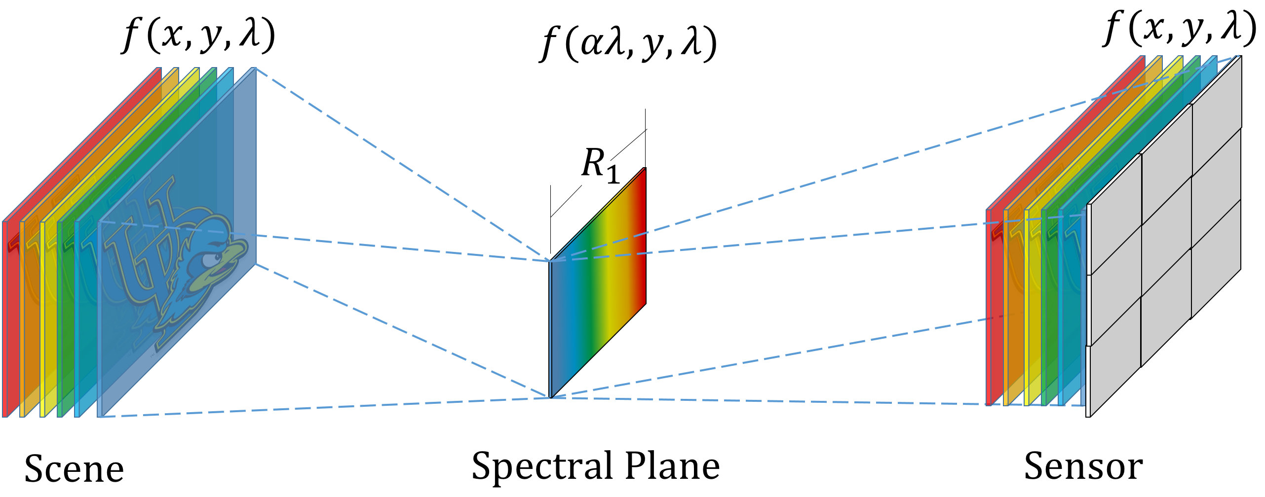 Figure 1
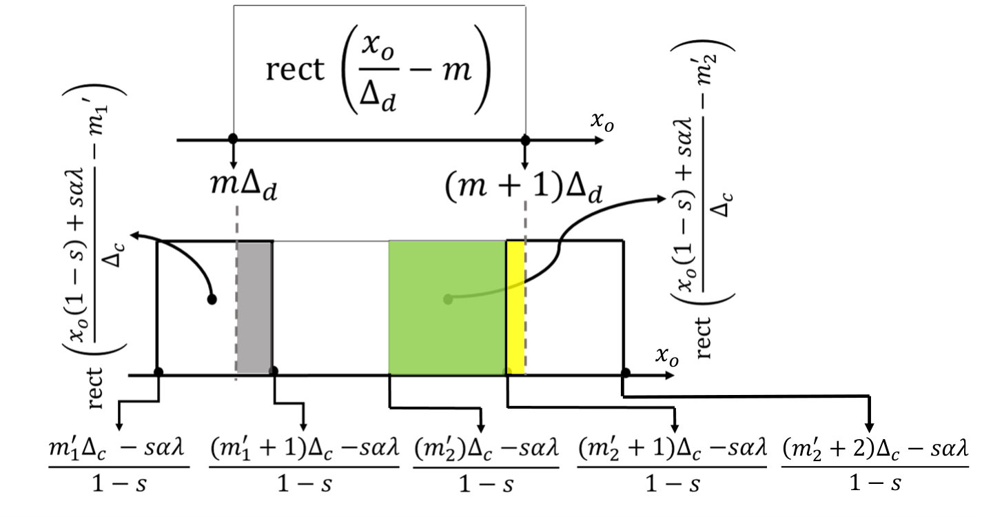 Figure 2
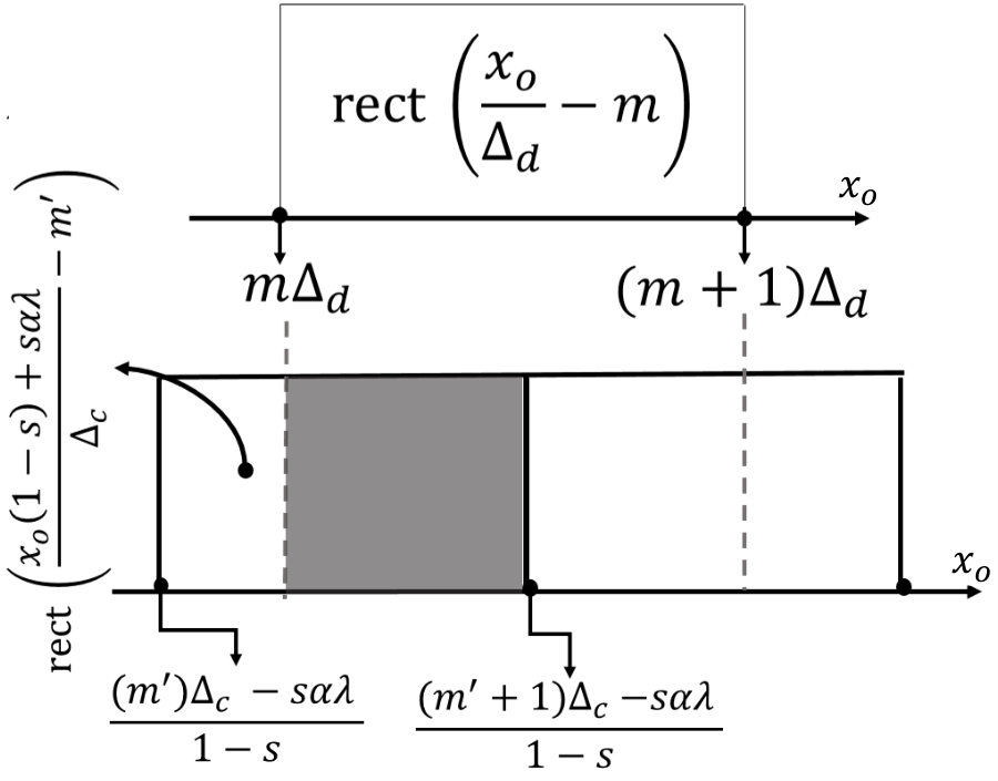 Figure 3
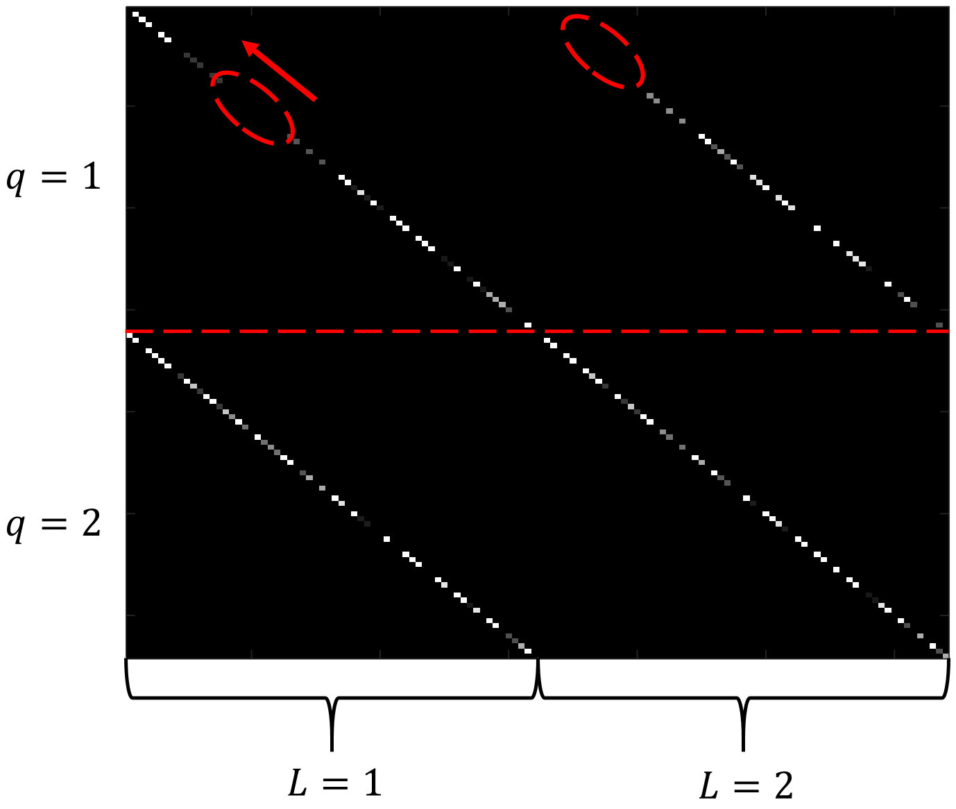 Figure 4
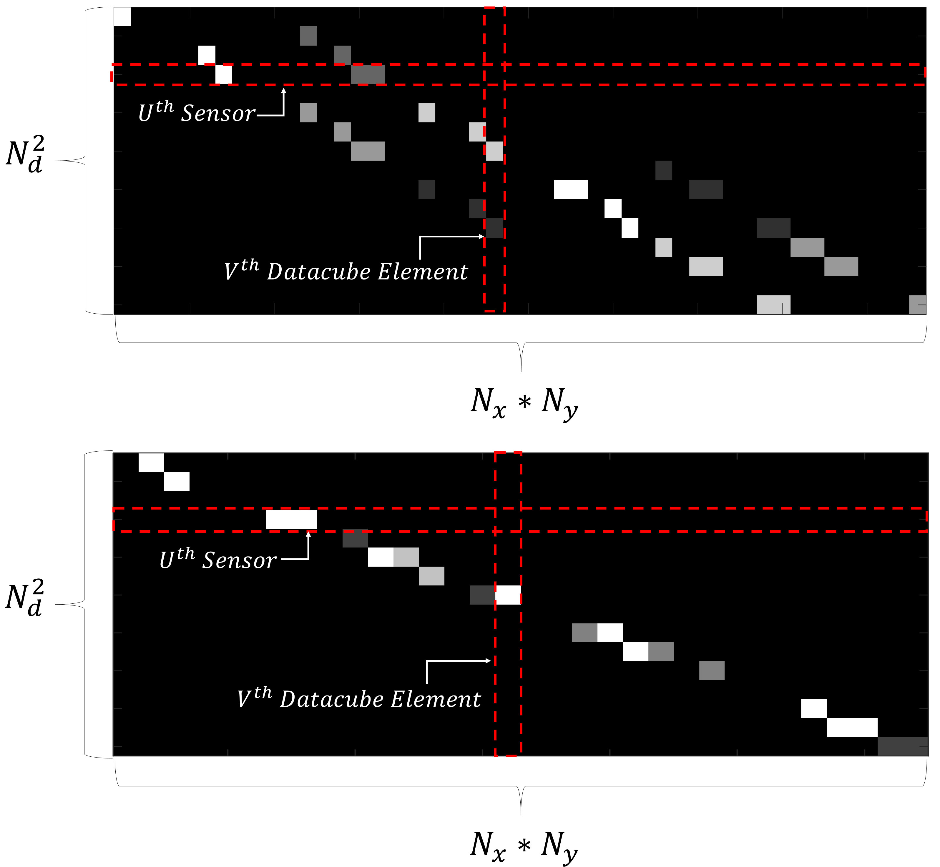 Figure 5
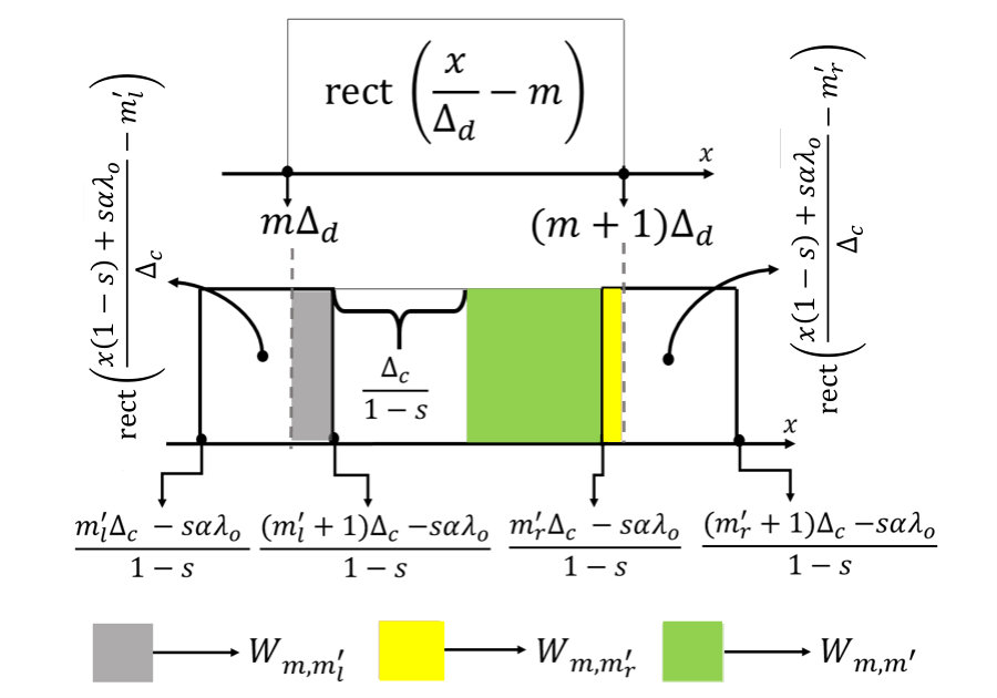 Figure 6
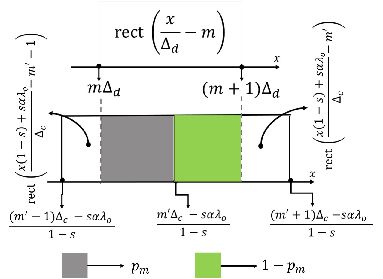 Figure 7
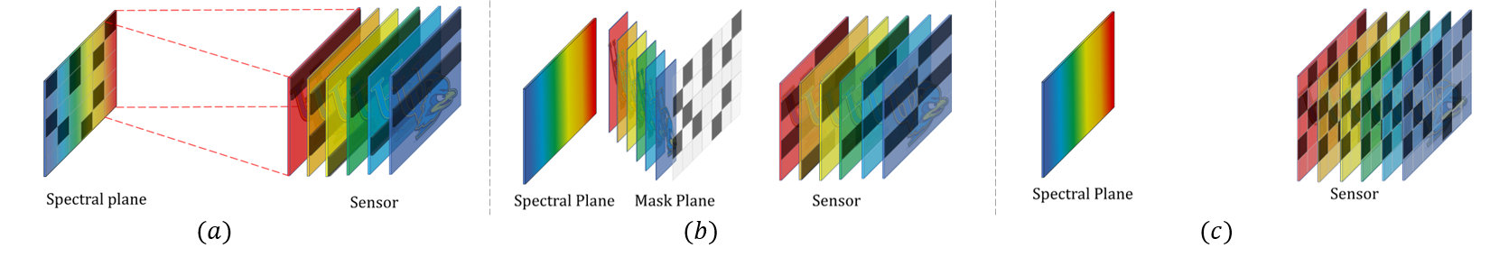 Figure 8
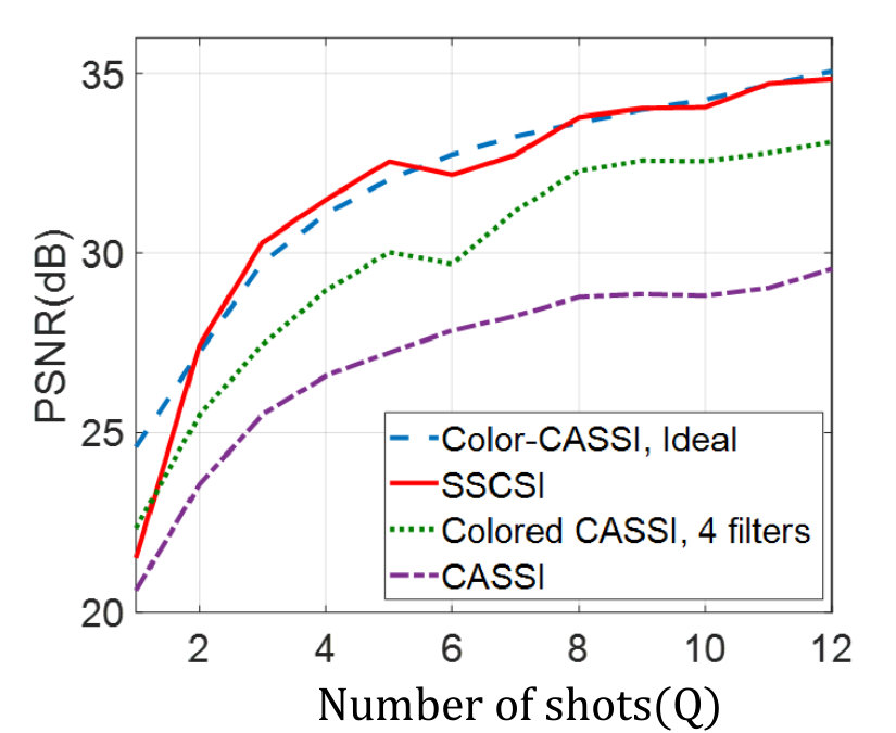 Figure 9
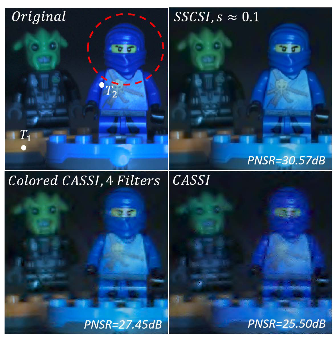 Figure 10
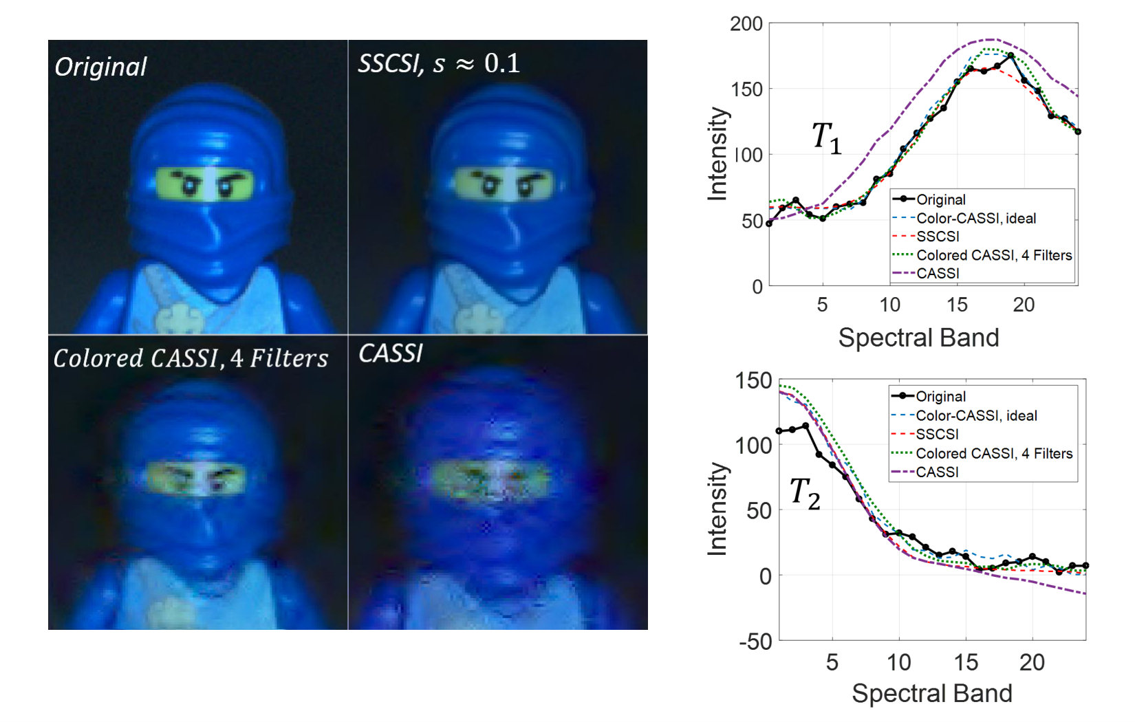 Figure 11
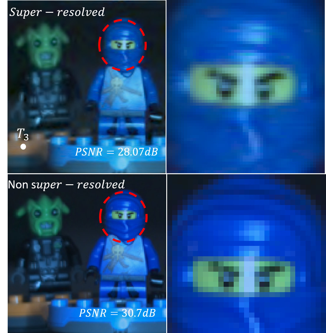 Figure 12
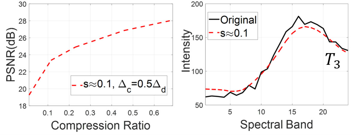 Figure 13
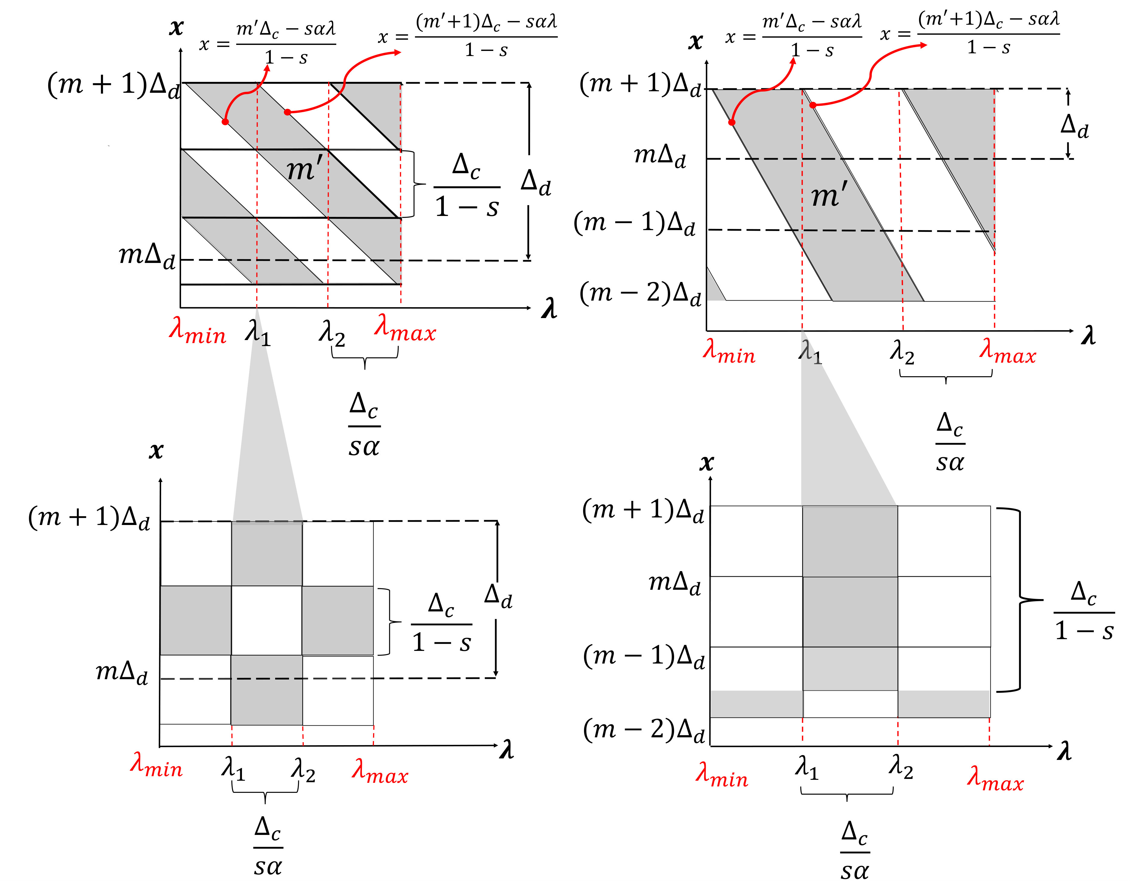 Figure 14
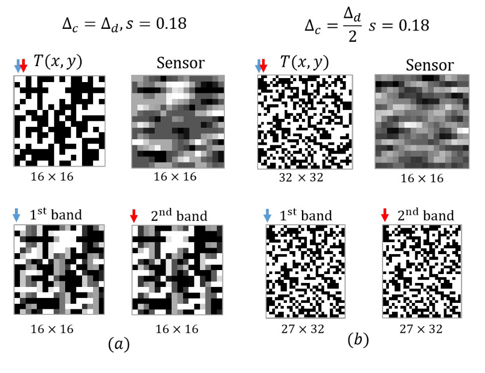 Figure 15
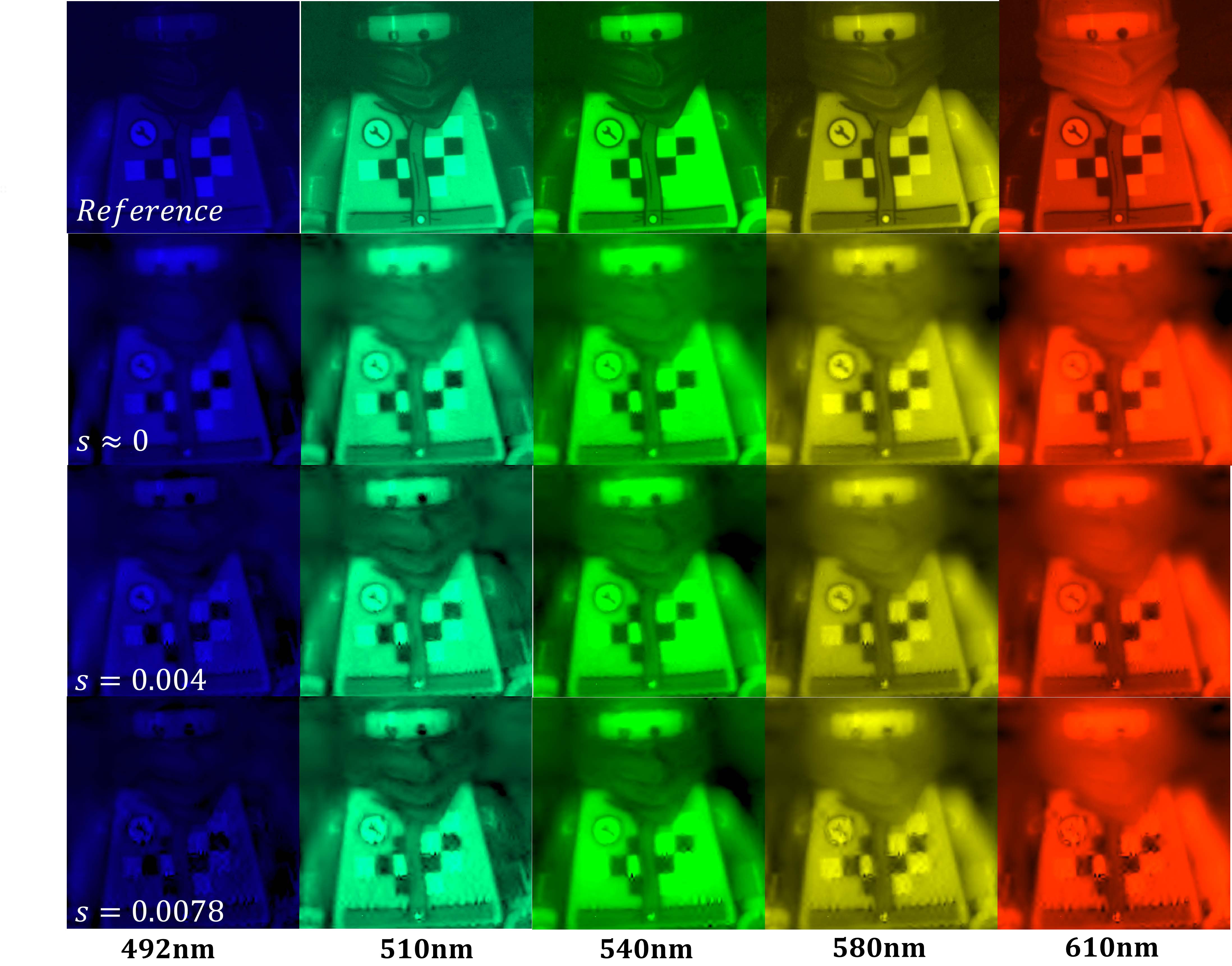 Figure 16
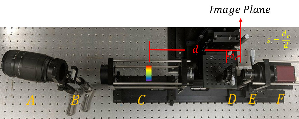 Figure 17
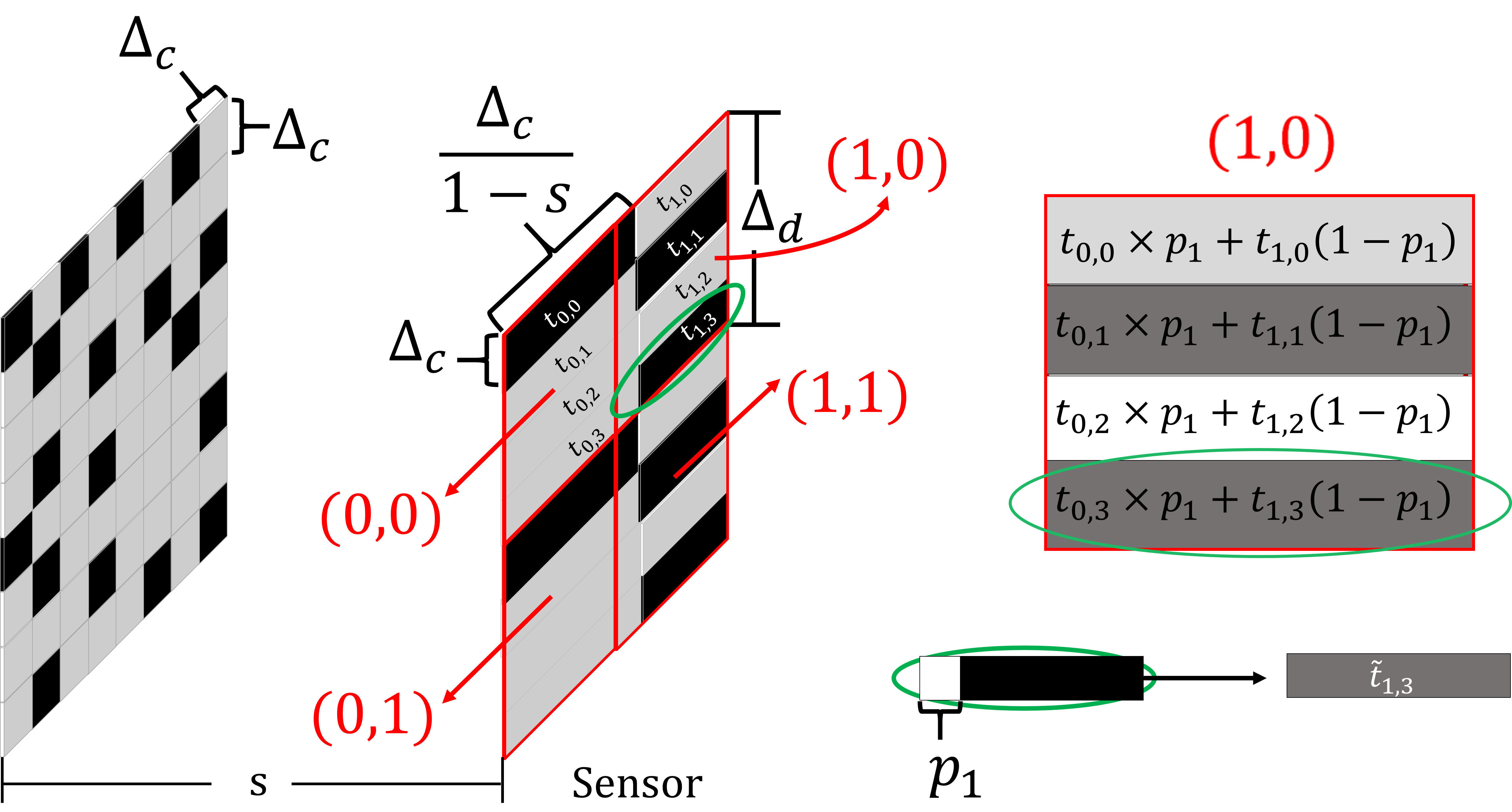 Figure 18
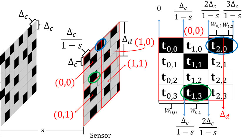 Figure 19
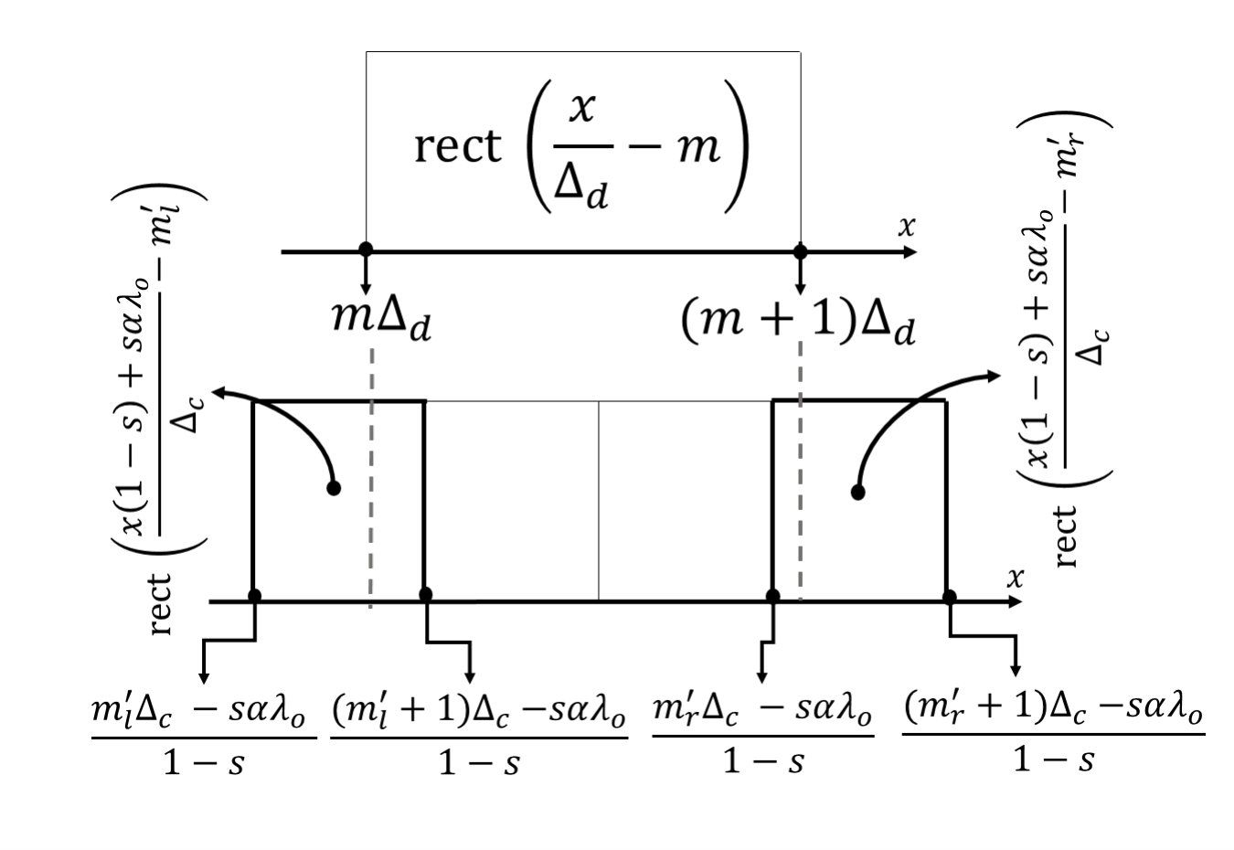 Figure 20
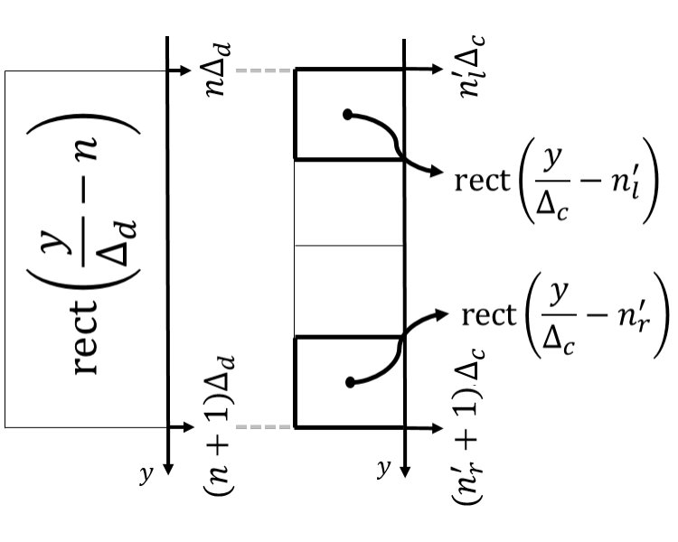 Figure 21
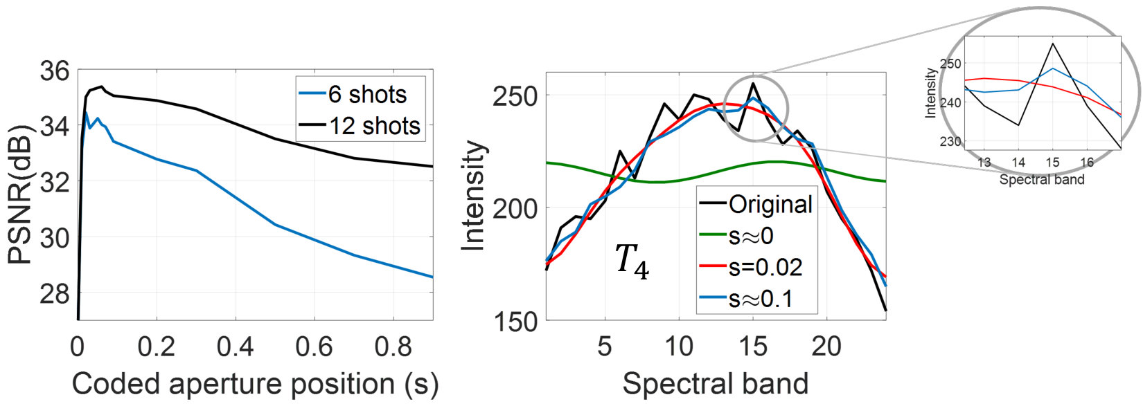 Figure 22
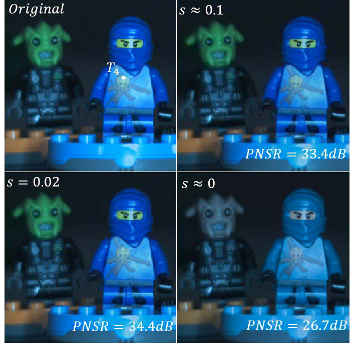 Figure 23
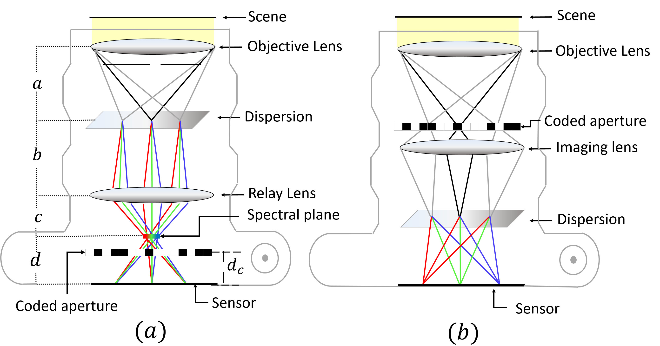 Figure 24
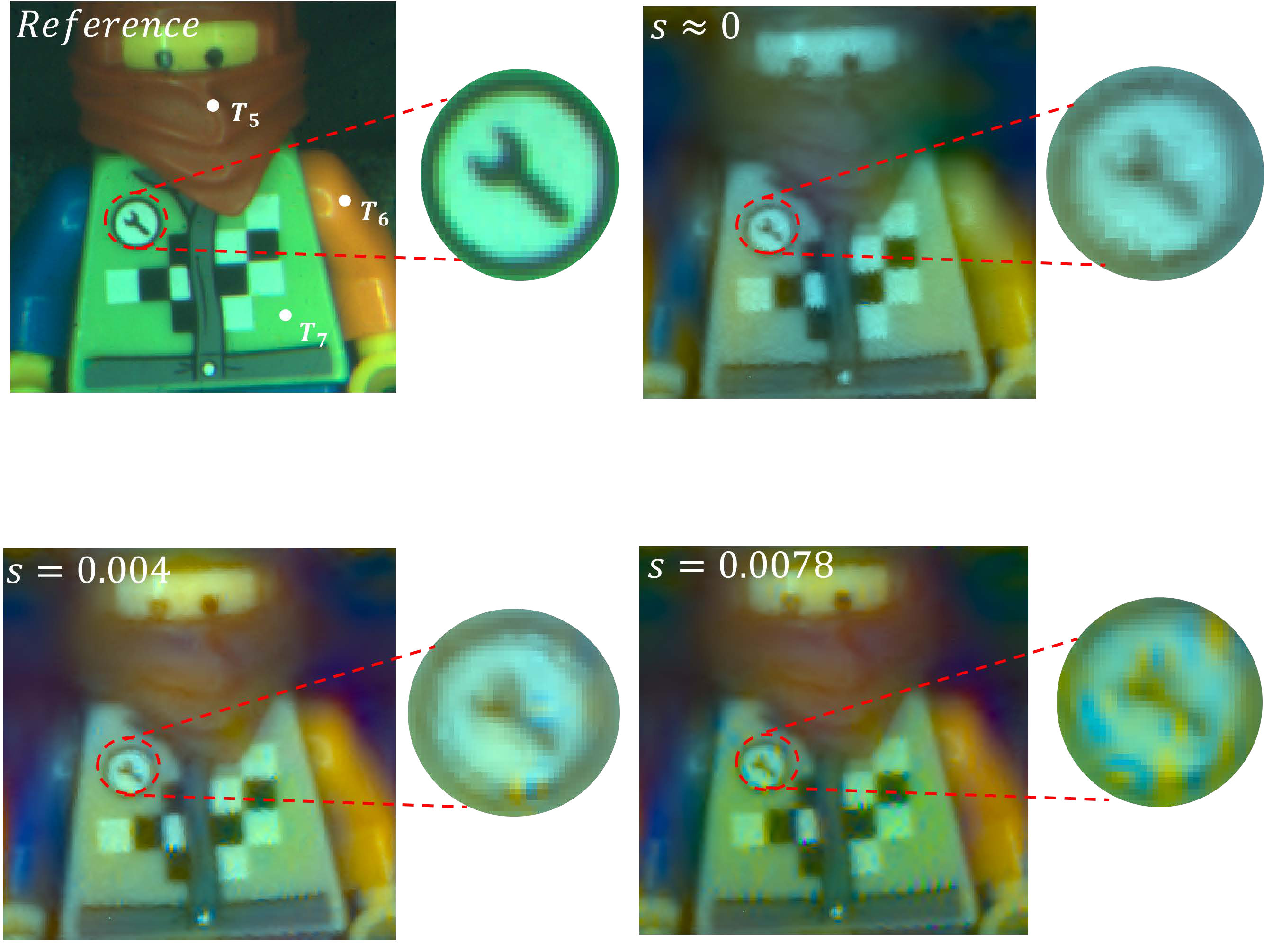 Figure 25
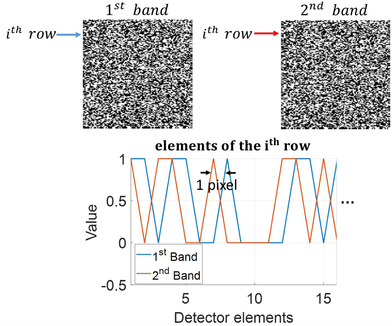 Figure 26
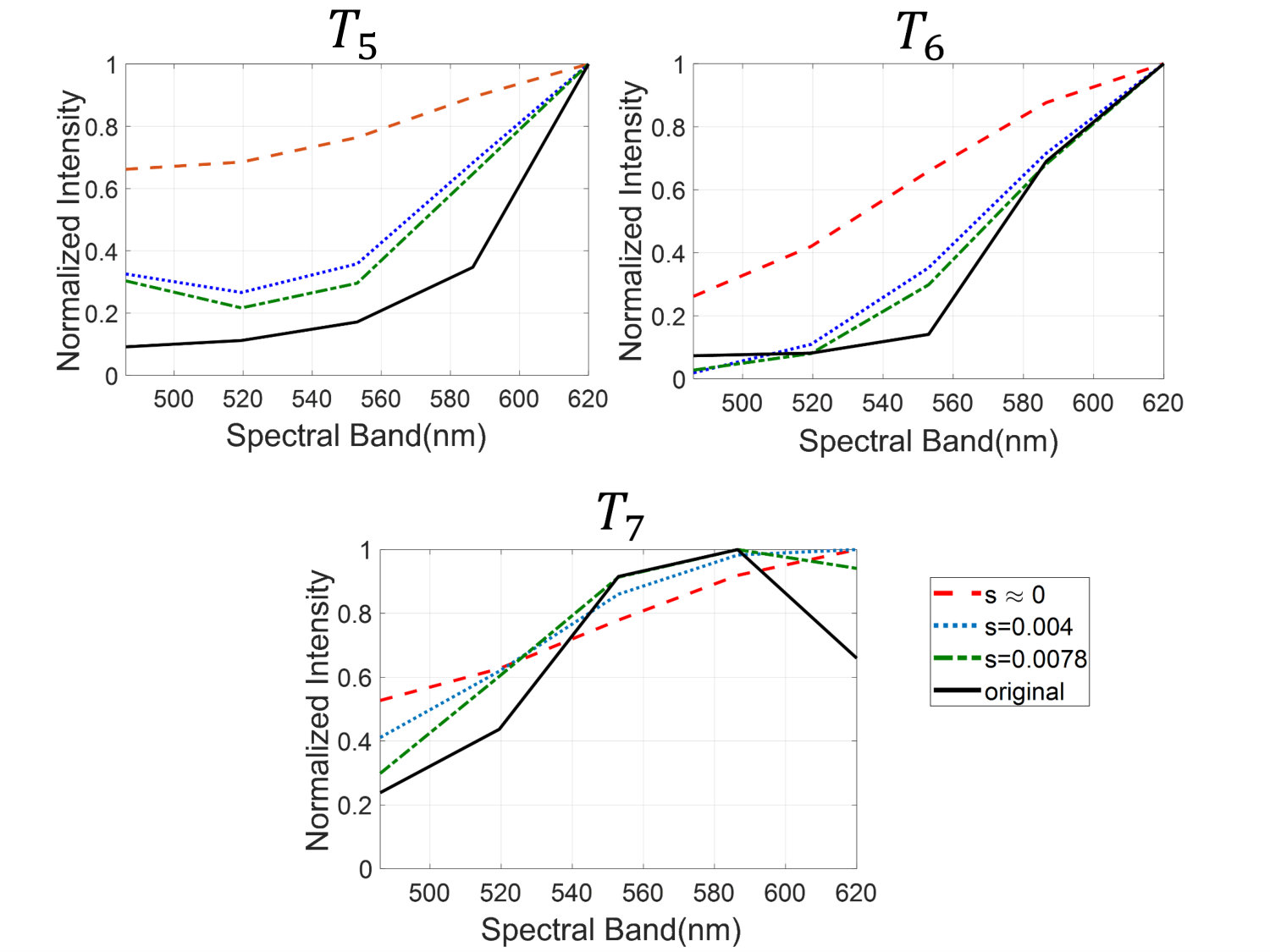 Figure 27
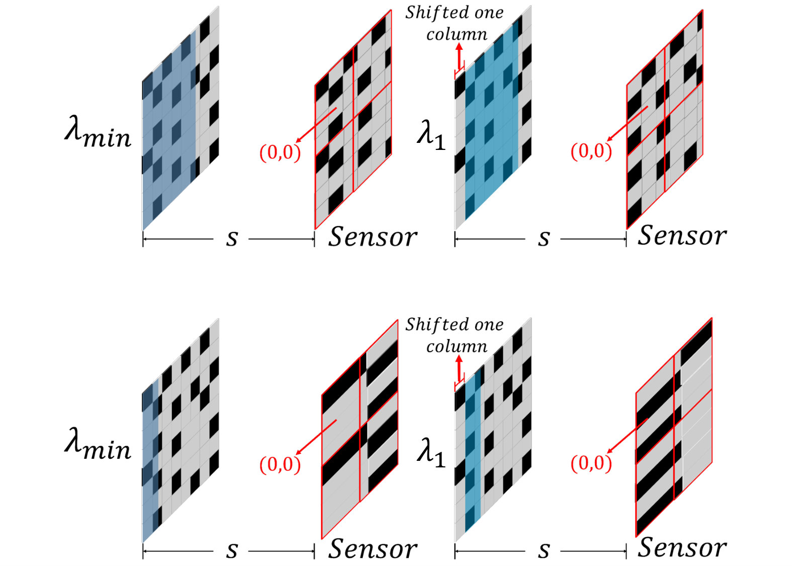 Figure 28
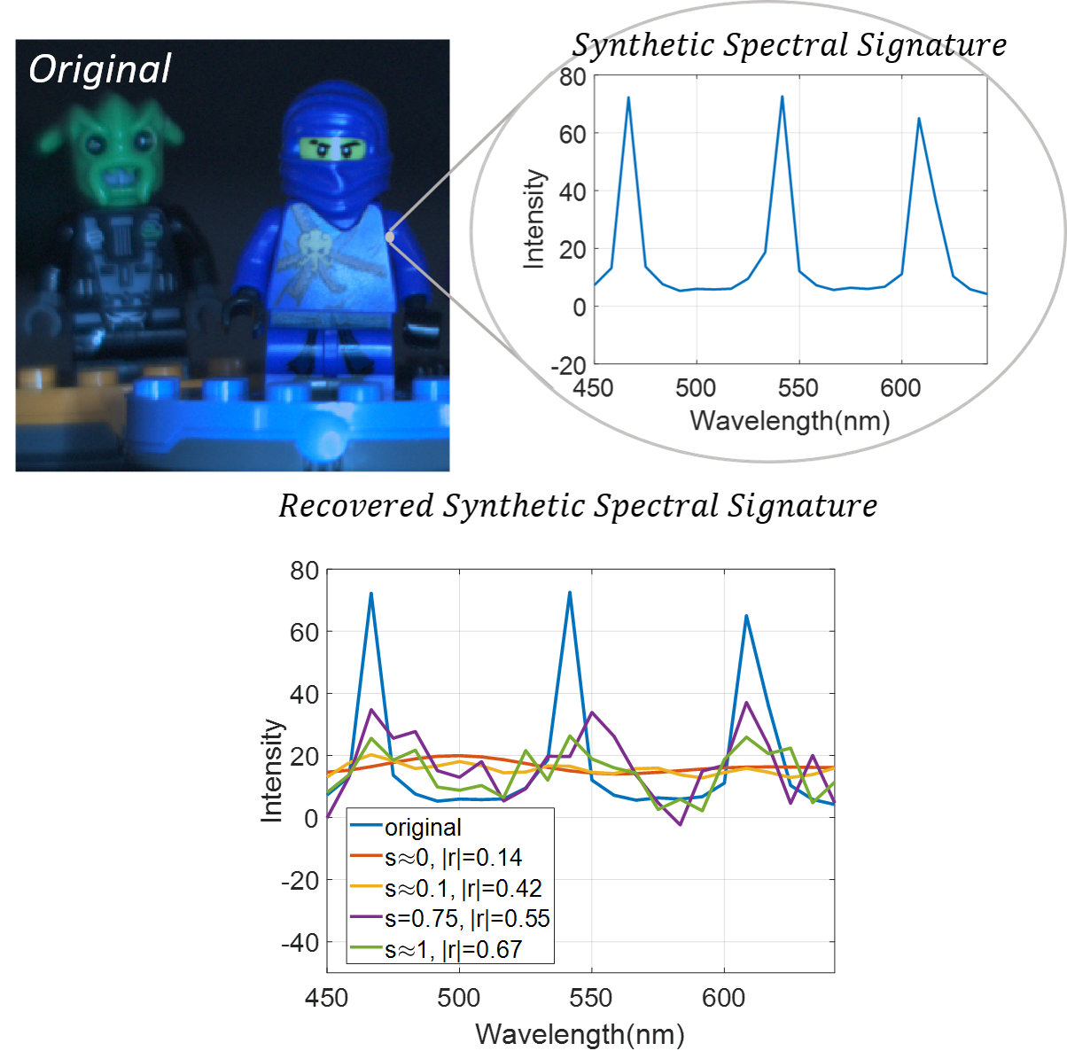 Figure 29
| s | PSNR(dB) | |
|---|---|---|
| 0 | 26.7 | 1 |
| 0.01 | 28.53 | 0.997 |
| 0.02 | 30.22 | 0.971 |
| 0.03 | 30.35 | 0.971 |
| 0.05 | 30.71 | 0.922 |
| 0.07 | 31.54 | 0.888 |
| s | , Theoretical (nm) | , Experimental (nm) |
|---|---|---|
| 0.004 | 43 | 40 |
| 0.0078 | 22 | 28 |
| 0.011 | 16 | 20 |
Peer Reviews
No public reviews on file for this paper yet. If you reviewed it on a platform where reviews are public (OpenReview, ICLR, NeurIPS, ICML), you can paste yours below so the community can read it here.
Videos
No videos yet. Explain this paper in a talk, walkthrough, or lecture? Add one.
Spectral Zooming and Resolution Limits of Spatial Spectral Compressive Spectral Imagers
Edgar Salazar, Alejandro Parada-Mayorga and Gonzalo R. Arce
Abstract
The recently introduced Spatial Spectral Compressive Spectral Imager (SSCSI) has been proposed as an alternative to carry out spatial and spectral coding using a binary on-off coded aperture. In SSCSI, the pixel pitch size of the coded aperture, as well as its location with respect to the detector array, play a critical role in the quality of image reconstruction. In this paper, a rigorous discretization model for this architecture is developed, based on a light propagation analysis across the imager. The attainable spatial and spectral resolution, and the various parameters affecting them, is derived through this process. Much like the displacement of zoom lens components leads to higher spatial resolution of a scene, a shift of the coded aperture in the SSCSI in reference to the detector leads to higher spectral resolution. This allows the recovery of spectrally detailed datacubes by physically displacing the mask towards the spectral plane. To prove the underlying concepts, computer simulations and experimental data are presented in this paper.
I Introduction
Hyperspectral imaging allows the simultaneous acquisition of spatial and spectral information of a given scene. It finds applications in a variety of fields such as remote sensing, medical imaging, food quality and spectroscopy [1, 2, 3]. As an alternative to the conventional hyperspectral sensing methods (push-broom, whisk-broom), the Coded Aperture Snapshot Spectral Imager (CASSI) [4, 5, 6, 7] was introduced; this is a Compressive Sensing based architecture [8], where the entire spatial-spectral datacube can be recovered from a few sensor measurements. A recently proposed enhancement of CASSI, replaces the binary on-off coded aperture by a pixelated color filter mask to achieve three dimensional coding prior to the optical sensing. This imager, known as colored CASSI [9, 10, 11, 12], increases both the quality of the reconstruction in the spatial domain and the attainable spectral resolution. Additionally, fewer snapshots are required to obtain accurate results [9]. The Snapshot Colored Compressive Spectral Imager (SCCSI)[13] and [14], on the other hand, represents a more compact version of the colored CASSI with remarkable performance, where the coded aperture is directly located on top of the sensor. Despite the advantages of both the colored CASSI and the SCCSI, the high fabrication cost of pixelated colored coded apertures limits their implementation in practice[15].
Recently, Lin et al. [16] proposed a new optical architecture called Spatial Spectral Compressive Spectral Imager (SSCSI). In this system, the spectral plane phenomena is exploited in order to carry out a three dimensional coding of the hyperspectral scene using a binary on-off mask. The spectral plane, see Fig. 1(a), is defined as the location where all the rays coming from the same wavelength meet each other in a single spatial point [17]. The SSCSI was first introduced as an attempt to replicate the functionality of the dual disperser CASSI, avoiding the calibration challenges, [18] and [19]. Coding in three dimensions, without the need of a colored mask, leads to high quality reconstructions while maintaining a low fabrication cost. Figure 1 depicts the ray tracing diagram of the SSCSI and the single disperser CASSI. The SSCSI system can be seen in Fig. 1(a), where the spatial-spectral coding process takes place after the spectral dispersion, and an in-focus image impinges on the sensor. In CASSI (see Fig. 1(b)), the coded aperture modulates an in-focus image of the scene and the dispersion occurs after the code modulation.
Some comparisons of the SSCSI with the different compressive spectral imagers have been done recently (Marín et al. in [20] and Medina-Rojas et al. in [21]). Nevertheless, a rigorous analysis of the SSCSI has not been developed, particularly on the resolution limits and the various parameters affecting the quality of the recovered scene. This paper provides such analysis with respect to the coded aperture and detector pitch sizes. Based on the continuous model studied in [16], a discrete expression of the sensor measurements is obtained. It is shown in section V-B and V-C, that spatial super-resolution is achievable, and a spectral zooming process can be done by displacing the coded aperture towards the spectral plane. Here, the term spectral zooming refers to the increment of the number of resolvable spectral bands on the recovered scene. This model is compared, by numerical simulations, against CASSI and colored CASSI in terms of spatial and spectral accuracy in the reconstruction. Additionally, a set of testbed experiments is performed in order to validate the underlying concepts. Some preliminary results of this research are described in [22] and [23].
This paper is organized as follows. In Section II, a description of the continuous model of SSCSI is presented. Section III presents the discretization of this model, offering a detailed description of the operators involved in the process. The structure of the sensing matrix is described in Section IV and the numerical simulations are presented in Section V. Sections VI and VII contain the experimental results and the conclusions, respectively.
II Sensing phenomena in SSCSI
This section contains the description of the sensing process for the SSCSI, developed in [16]. The SSCSI optical architecture depicted in Fig. 1(a), makes use of an objective lens to locate an image of the scene directly on the diffraction grating, where the spectral dispersion takes place. The rely lens is then used to get an in-focus image onto the sensor. Figure 2 depicts the ray propagation of the scene onto the spectral plane and into the sensor. Notice how all rays from a same wavelength converge to a single line on the spectral plane. The width of that spectral plane, , is given by the following expression [17]
[TABLE]
where is the distance between the grating and the relay lens and is the distance between the spectral plane and the sensor (see Fig. 1(a)). The variable is the grating dispersion angle.
The parameter (see Fig. 1(a)), represents the position of the coded aperture with respect to the sensor. This normalized variable ( when the coded aperture is on top of the sensor and when the coded aperture is on the spectral plane), strongly affects the coding process happening on the SSCSI. As depicted in Fig. 3(a), when each resolvable spectral band will be coded by a different column of the mask and a stretched version of the coded aperture will impinge on the sensor. When (see Fig. 3(b)) a similar process occurs, but in this case each resolvable band will be coded by a bigger portion of the coded aperture. When , on the other hand (see Fig. 3(c)), all the spectral information will be coded by the same coded aperture pattern. As it will be described shortly, the parameter plays a crucial role in the resolution limits of SSCSI. The sensing process of the hyperspectral scene after being coded at a given , is characterized by the following expression [16]
[TABLE]
where is the continuous model representation of the information captured at the sensor (see Fig. 2), is the coded aperture function, is the continuous representation of the hyperspectral scene, is a parameter that indicates the position of a given wavelength on the spectral plane (see Appendix D for more details), and is the spectral range of interest, typically going from nm to nm [16]. Notice how the term appears on the argument of , which reflects the dependency of the coding process on that parameter. In this expression, it is assumed that the aperture of the objective lens is an infinitesimally small pinhole; however, in practice, an aperture with finite dimensions will introduce blurring effects as it will be explained in Section VI. Given that the sensor is composed of a discrete array of elements, a discretization process of Eq. (2) is a crucial step in understanding the physical phenomena in terms of the real captured information; this will be done in the following section.
III Discretization of the sensing phenomena
This section contains the steps followed in order to find a discrete expression for the captured data in the SSCSI. The discretization is performed based on the analysis of the product of the rectangular functions that represent both the coded aperture and the detector. The spatial resolution limits are first analyzed by assuming a single wavelength scene. This leads to a discrete measurement expression that is posteriorly extended to a multiple wavelength hyperspectral scene, by defining the spectral resolution limits on the SSCSI.
Consider the pixel detector, where are integer and unitless values, and are the dimensions of the sensor array. The captured data on can be written as follows
[TABLE]
where is the pitch size of a single detector element and is a rectangular function defined as follows
[TABLE]
Likewise, the coded aperture can be written as
[TABLE]
where , are integer and unitless values, and are the dimensions of the coded aperture mask. The variable is the pitch size of the coded aperture. In this paper, the coded aperture full width is assumed to be the same as the detector full width, or . Moreover, the detector and the mask are assumed to be totally aligned with respect to each other. Replacing (5) into (3) leads to
[TABLE]
A discretization measurement model of the last equation implies first a rigorous analysis of the spatial and spectral resolution limits related to the SSCSI, which will be done in the next subsections.
III-A Spatial Resolution Limits
Consider a spectral scene having just one spectral component, where is a Delta Dirac function located at . Equation (6) can be rewritten as
[TABLE]
By solving the integral over , Eq. (7) can be rewritten as
[TABLE]
The minimum spatially resolvable feature, given by Eq. (8) can be determined by establishing the intersecting region of the two rectangular functions in that expression. As it will be explained, this region is going to depend on the size of a coded aperture pixel projected onto the sensor.
III-A1 When
Figure 4 left illustrates the coded aperture at a given position and its projection onto the sensor; the red lines delimit the detector elements. As depicted, a single coded aperture pixel of dimensions is mapped into a rectangle on the detector. This area defines the attainable spatial resolution of the recovered scene, as long as . In this paper, it is assumed that and that the ratio is an integer greater than or equal to 1 (see Appendix E for ); this last condition implies that the mismatch between the coded aperture and the detector only applies to one axis (see Fig. 4, blue circled region).
Let and be the upper-leftmost and lower-rightmost coded aperture elements impinging on the detector element. The overlapping of the two rectangular functions in Eq. (8) can be seen in Figs. 5 and 6. From Fig. 5, it can be inferred that for the overlap to exist on the axis, the following condition must hold
[TABLE]
where the limits in the last inequality come from solving and for and respectively. Likewise, it can be shown based on Fig. 6, that for the two rectangular functions in Eq. (8) to overlap in the axis, the next condition must hold
[TABLE]
where is the floor operator. The limits in the last inequality come from solving and for and respectively and considering that and are integer indexes. Given that the minimum resolvable spatial feature is of dimensions , and that the overlapping regions of the rectangular functions in Eq. (8) are defined in (9) and (10), the captured information in the detector element, , can be represented as
[TABLE]
where and are the limits of the expression in (10) and the variable is the datacube representation of the hyperspectral scene, being the information of the datacube at position and spectral band ; is obtained by applying the integral operators in Eq. (8). Notice that the spatial dimensions of , using an sensor array, are defined as , where is the ceiling operator. The parameter is the fraction of the coded aperture element impinging on the detector element, and it is defined as follows (see Appendix A for full derivation),
[TABLE]
A similar analysis was previously done for the CASSI system by Galvis et al. [24], in order to model the mismatching between the coded aperture and the sensor array. As an example, take the sensor element in Fig. 4 right; the captured information in this element will be equal to . In this particular case and .
III-A2 When
The projection of the coded aperture onto the sensor when is as shown in Fig. 7 left. Unlike the last scenario, the attainable spatial resolution in the axis is limited not by but by the detector pitch size ; the minimum spatially resolvable feature is then of dimensions . As when , a coded aperture-sensor mismatch is present. To deal with this particularity, a synthetic effective pattern is generated by the combination of elements proportional to the areas, as illustrated by the green circle in Fig. 7 right.
Given the coded aperture pixel and the detector element, the two rectangular functions in Eq. (8) intersect each other if falls on the interval specified in (9) and (see Appendix A). Taking into account that the minimum spatially resolvable feature is of dimensions , the captured information in a particular sensor element, , can be written as follows
[TABLE]
where is obtained by applying the integral operators in Eq. (8). Notice that the spatial dimensions of , using an sensor array, are defined as . The expression represents the effective coded aperture, where indicates the percentage occupied by on the detector element and is defined as follows (see Appendix A),
[TABLE]
Unlike , that represents a percentage value with respect to a coded aperture pixel, is a percentage value with respect to the detector pitch size . As an example, take the sensor element in Fig. 7 right. The captured information in this particular case will be equal to:
Now that the spatial resolution limits were defined, an analysis to determine the minimum resolvable spectral band on the SSCSI must be developed in order to extend the discretization models, given in Eqs. (11) and (13), to the multi-spectral case.
III-B * Spectral Resolution Limits*
A similar process to the one done to calculate the spatial resolution must be done to find an expression for the spectral resolution in SSCSI. In this case, a multispectral scene representing a single spatial location, where is a two dimensional Delta Dirac function located at , is going to be considered. With this assumption, Equation (6) can be rewritten as follows
[TABLE]
By solving the integral over , Equation (15) can be rewritten as
[TABLE]
The attainable spectral resolution of the SSCSI is determined by the intersecting region of the two rectangular functions in Eq. (16). It can be shown that when , that region has a length of for certain values of (see Appendix B). Therefore, the maximum number of resolvable spectral bands is given by
[TABLE]
where is the spectral range of interest. Notice that the term indicates the spectral dispersion of the datacube for a given position . Let and be two wavelengths, such that . The dispersion between these two bands is given by . This means that two adjacent and resolvable bands will be coded by the same coded aperture but shifted by one column as depicted in Fig. 8, top (for ). Eq. (11) can therefore be extended to the multispectral case as follows
[TABLE]
where , and is defined in Eq. (12) (for ). The spectral band is defined here as the interval ; the shifting by one column between adjacent bands can be seen in the term on the coded aperture array . The dimensions of the recovered datacube are given by , where are the dimensions of the sensor array and is given in Eq. (17). As an example, take the sensor element in Fig. 8, top; the captured information in that element related to the spectral band will be given by . Likewise, the captured information for the spectral band will be given by . Notice that in this particular case, . Since the actual shearing of the coded aperture seen at the sensor is approximated, this model can be called First order approximation. An analysis of the actual sheared coded aperture pattern and the parallel with the proposed model can be found in Appendix C.
When , a similar analysis can be done to find that the attainable spectral resolution can be assumed as (see Appendix B). Again, as when , two adjacent and resolvable bands will be coded by the same coded aperture but shifted by one column, or , as depicted in Fig. 8, bottom (for ). Eq. (13) can therefore, be extended to the multispectral case as follows
[TABLE]
where the spectral band is defined as the interval , and is as defined in Eq. (14) (for ). The shifting by one column between adjacent bands can be seen in the term on the coded aperture array . The dimensions of the recovered datacube are given by , where is given in Eq. (17). As an example, take the sensor element in Fig. 8, bottom. The captured information in that element related to the spectral band will be given by . Likewise, the captured information for the spectral band will be given by . Again, the present model is an approximation and an analysis of the actual sheared coded aperture can be seen in Appendix C.
Figure 9 shows the coded aperture projected onto the sensor and the equivalent coded aperture for two adjacent bands when and . Notice that the recovered datacube might not be square, as the resolution in each spatial axis can be different.
The dependency of the number of resolvable bands on and , as stated in Eq. (17), allows to enhance the spectral resolution of the system by tunning these parameters. Increasing , which means moving the coded aperture towards the spectral plane, is equivalent to do a zooming process over the spectral dimension of the datacube. However, in experiments, placing the coded aperture at decreases the spatial resolution of the recovered scene. This will be further discussed in the experimental part of the present paper.
An alternative expression for the number of the resolvable bands can be seen in the following equation (see Appendix D for full derivation),
[TABLE]
where is the ratio between the width of the spectral plane and the coded aperture full width. If , the spectral plane fully occupies the coded aperture width. The variable is related to , given by Eq. (1); therefore, a convenient way to increase is choosing a diffraction grating element with high diffraction angle .
IV Matrix Forward Model
Given the discrete measurement model explained in the previous section, the sensing process can be expressed in a matrix form as follows
[TABLE]
where is the number of captured shots and is the column-wise version of the measurements of length . The variable is a column-wise sparse representation of the datacube in a basis . If the datacube to be recovered has dimensions , then the length of is . The structured matrix performs the coding process of the datacube; its dimensions are . Figure 10 shows the structure of when and for a single wavelength datacube. Each row of corresponds to a sensor element, while each column corresponds to a datacube component. The values of the nonzero entries of the matrices are linked to Eqs. (18) and (19). Notice that one single sensor can measure several datacube elements.
For a multishot approach, the sensing process can be written as
[TABLE]
where is a structured matrix with dimensions , and is a vector of length . The structure of for and can be seen in Fig. 11. Unlike CASSI, the dispersion in the SSCSI is seen as the movement of the elements on the diagonals. An example on how to ensemble when and the coded aperture has the same dimensions than the detector , can be seen in Algorithm 1. In this particular case, according to Eq. (9), . The computational complexity of this algorithm is . When , a similar process to the one specified in Algorithm 1 must be done. In this case, for every detector element, , and is calculated using Eqs. (9) and (10) and (12).
V Simulations
This section contains the simulation results in order to test the SSCSI first order approximation. The model is first compared to CASSI in terms of spatial and spectral quality in the reconstructions. After that, the spatial super-resolution and the spectral zooming concepts are tested in simulations. The performance of the SSCSI at different values of is then analyzed. A last subsection regarding the coherence of the sensing matrix and the impact on the quality of the reconstruction, is included. A hyperspectral scene was captured at the Computational Imaging and Spectroscopy Laboratory at University of Delaware, using a visible monochromator between 451nm and 642nm and a CCD camera, to posteriorly implement it as a ground-truth in simulations. The sparsity basis was chosen as , where is the 2D Wavelet Symlet 8 basis, is the Discrete Cosine basis and is the Kronecker product [25]. The reconstruction is obtained as the solution of
[TABLE]
where is the norm, is the norm, is a regularization parameter that controls the sparsity of the solution and . The Gradient Projection for Sparse Reconstruction algorithm (GPSR) is used in order to solve Eq. (23), as this algorithm has been shown to have optimal numerical performance and speed [26].
V-A Comparison to CASSI and Colored CASSI
The recovery process of a hyperspectral scene with bands was simulated with a detector array, with , and using the CASSI, the colored CASSI and the SSCSI first order approximation developed in this paper. Since , for any value of . Therefore, the spatial size of the recovered datacube is going to be , with . Given that bands must be recovered, the coded aperture must be located at , according to Eq. (20) and assuming that . The fact that means that impinges in the leftmost side of the coded aperture and impinges on the rightmost side of the coded aperture, or . The codes were generated such that the information captured in the shots is complementary, where the term complementarity is characterized by the condition ; this structure, called Boolean, has been proven to be optimal for the CASSI architecture [27]; the transmittance of every coded aperture with boolean structure is inversely proportional to the number of captured shots. The regularization parameter was empirically chosen to attain optimal results for all the scenarios, being in the majority of cases between and . The Peak Signal-to-Noise Ratio (PSNR) was the parameter implemented in order to determine the quality of the reconstructions. The PSNR is defined as , where is the maximum possible value of the image and is the mean squared error with respect to the ground-truth. Figure 12 shows the PSNR of the reconstructed scene as a function of the number of shots for the CASSI, the SSCSI first order approximation and the colored CASSI. The colored CASSI was implemented in two ways; in the first one, the coded aperture patterns were chosen such that the condition holds, with no limitation on the type of optical filters; this is called ideal colored CASSI. In the second one, the types of filters are limited to four: low pass, high pass, band pass and band stop, and the patterns on the mask were chosen such that the condition holds. Here, represents the component of the spectral response of the optical filter located at position and shot . As depicted, the SSCSI exhibits much better performance than both, the CASSI and the colored CASSI with 4 filters while achieving similar results to the ideal colored CASSI. The comparison between the original scene and the recovered datacubes for snapshots can be seen in Fig. 13, while a zoomed version can be observed in Fig. 14 left. Here, the hyperspectral scenes were mapped to the RGB domain for visualization purposes. A comparison between the original and recovered signatures for two different pixels, can be seen in Fig. 14 right. As depicted, the SSCSI, the ideal colored CASSI and the colored CASSI with 4 filters show spectrally accurate results.
V-B Spatial Super-Resolution
In [28], Arguello et al. proposed the reconstruction of spatially super-resolved hyperspectral scenes using CASSI, assuming that the ratio is an integer greater than 1. Likewise, with the SSCSI, Eq. (18) allows the reconstruction of spatially super-resolved datacubes with dimensions . Consider and a detector array, with ; with the SSCSI, a super-resolved datacube of spatial size and spectral bands, can be recovered if the coded aperture is located at and . Figure 15 top left and right, shows the recovered super-resolved datacube when the compression ratio is . The compression ratio, , is defined as the ratio between the number of captured measurements and the size of the reconstructed datacube, or . Here, is the number of detector elements and is the size of the recovered datacube. The value of must be less than in order to have compression during the capturing process. The non super-resolved datacube obtained from the same detector array can be seen in Fig. 15 bottom left and right. A simple inspection of the target reveals the effect of the super-resolution on the spatial details of the reconstruction. The PSNR of the reconstructed super-resolved datacube as a function of the compression ratio can be seen in Fig. 16 left. Here, the compression ratio is incremented by increasing the number of captured snapshots . A comparison between the original and the recovered spectral signatures can be seen in Fig. 16 right.
V-C Spectral Zooming
To illustrate the zooming process over the spectral dimension in a given scene, a spectral signature with strong peaks on three different wavelengths was introduced in the original datacube; the recovery was done for different values of and a compression ratio of . The conditions of , and boolean coded apertures were assumed. As illustrated in Fig. 17, no spectral details can be identified when the recovery is done at or ; when and , on the other hand, the recovered spectral signatures are closer to the original one. This closeness is measured by the absolute value of the correlation coefficient , between the original and reconstructed signatures.
V-D Performance at different
As previously explained in section V-A, to recover a hyperspectral scene of bands using an sensor, with , and , one must locate the coded aperture at , if . This subsection analyses the impact of recovering that same scene for different values of . Figure 18 shows the RGB profiles of the recovered scene for three different values of and snapshots. It is clearly seen that with , the colors of the scene do not properly match the colors of the original datacube.
Figure 19 left, shows the PSNR of the reconstructed hyperspectral scene as a function of the coded aperture position, for and snapshots. As depicted, if , the quality of the reconstruction is low, since the system is not able to distinguish any spectral information of the scene. Increasing leads to enhance the quality of the reconstruction. However, when gets close to , the PSNR drops as it was also shown in [16]. The comparison between the spectral signatures for different values of can be seen in Fig. 19 right; reducing to makes the fine details of the curve to be lost while maintaining its shape; for , no spectral information is recovered.
V-E Coherence of the sensing matrix
In compressive sensing, the coherence of the sensing matrix , where , has been extensively used as a measure of the quality of the sensing process, where matrices with a low coherence lead to high quality reconstructions [29, 30, 31, 32]. Table I contains the PSNR values of the reconstructions and the coherence of the sensing matrix for different values of . Here, a sensor array with was considered, with and . A multispectral scene of dimensions was recovered and the coded apertures exhibit boolean structure. As it can be appreciated in Table I, is connected to the quality of the recovered scene and low values of are associated to high PSNR values. Further analysis of the coherence in SSCSI will be done in future work.
VI Experimental measurements
The SSCSI was experimentally implemented as depicted in Fig. 20. A TAMROM AF 70-300mm lens locates an image of the scene at the transmissive diffraction grating (300 grooves/mm). The diffracted image is then reshaped using a 4f system composed of two 75mm, 2” lenses. In a 4f system, the image located at a distance with respect to the first lens is reshaped at a distance with respect to the second lens. The 4f system provides major flexibility in the movement of the coded aperture, in the sense that is accessible, since it is located in a spatial position far from the sensor. The spectral plane will be located in between the lenses that compose the 4f system. The coded scene is then reshaped at the sensor by a 1”, 35mm lens. The implemented sensor is a StingrayTM CCD monochrome camera with 9.9µm pitch size. The spectral range of interest was defined as 480nm-620nm.
VI-A Spectral Resolution
The theoretical spectral resolution can be determined by defining the size of the spectral plane with respect to the coded aperture ( in (20)). It was found that the 480nm-620nm spectral range occupies a physical space three times the coded aperture width, therefore, . This was done by locating a white board on the spectral plane and measuring the physical distance between nm and nm. The number of resolvable bands with and is given by . On the other hand, the criteria used to determine whether two adjacent spectral bands are resolvable in experiments, can be seen in Fig. 21. As depicted, the patterns that code two adjacent spectral bands at a given are first captured with the sensor; then, the rows from those patterns are compared. In order for the two bands to be resolvable, the curves must be shifted by one pixel. Table II shows the experimental and theoretical spectral resolution for different values of .
VI-B Experimental Datacube Reconstruction
A hyperspectral scene was reconstructed using snapshots and different values of . The coded aperture patterns exhibit boolean structure and were printed on a photo-mask with pitch size of µm. The matrix was generated by first locating a white board target and then capturing the coded aperture pattern for each spectral band to be recovered, at a given . Then, that pattern is located in the respective diagonal of the matrix ; this is done for every captured snapshot. After that, the white board is replaced by the hyperspectral scene, and the snapshots are properly captured. The reconstruction algorithm is posteriorly executed to find the optimal coefficients . The RGB profiles of the reference scene and the reconstructed datacubes can be seen in Fig. 22, while the spectral bands and recovered spectral signatures are contained in Fig. 23 and Fig. 24. As depicted, increasing allows the spectral information of the scene to be better distinguished.
The SSCSI bases its functionality on the location of the coded aperture in an out of focus position or , as depicted in Fig. 1. As mentioned in Section II, the present model assumes an infinitesimally small aperture in the objective lens. However, in experiments, the finite size of the aperture introduces blurring effects when and, in fact, increasing deteriorates the spatial quality of the reconstructed hyperspectral scene. Figure 22 shows the zooming over one portion of the recovered scene for the different values of . It is evident that the colors of the scene become more noticeable for a bigger , but at the same time, the spatial quality drops.
There are several factors to consider in the experiments. Besides the blurring proportional to , that affects the spatial quality of the reconstructions, one might find other challenges when implementing the SSCSI. One of them is the amount of light that passes through the system, since the aperture of the objective lens must be as small as possible. At the same time, the size of this aperture directly affects the resolution of the SSCSI, given that the minimum resolvable feature for any optical system is determined by the diffraction limit. On the other hand, the fact that the spectral plane is three times bigger than the coded aperture , leads to extreme wavelengths to impinge out of the mask; this means, in practice, that the range of wavelengths is reduced to the ones impinging inside the mask.
VII Conclusions and further steps
This papers develops a rigorous discretization measurement model of the Spatial Spectral Compressive Spectral Imager (SSCSI), based on the physical dimensions of the coded aperture and the detector array, and the spectral dispersion introduced by the diffraction grating, characterized by . Two different scenarios were proposed:
- •
: This scenario is modeled by Eq. (18), where is used to model the mismatch between the coded aperture and the detector array. The spatial resolution is defined as . As described in Section V-B, a spatially super-resolved datacube of dimensions, can be recovered when this condition holds.
- •
: This scenario is modeled by Eq. (19), where an effective mask is generated by the combination of coded aperture pixels proportional to the areas, using the variable . The spatial resolution is defined as
The number of spectral bands that can be recovered using the SSCSI was found to depend on three variables: The coded aperture pitch size , the spectral dispersion introduced by the diffraction grating characterized by , and the coded aperture position represented by the parameter . In fact, it was found that a bigger increases the number of resolvable spectral bands. Therefore, a movement of the coded aperture towards the spectral plane can be seen as performing a spectral zooming over a given hyperspectral scene. The SSCSI performance, in experiments, depends on the aperture of the objective lens. Increasing the size of the aperture makes the spatial quality of the recovered scene to drop as the coded aperture is displaced towards the spectral plane. On the other hand, reducing the aperture also decreases the amount of light passing through the system.
Ongoing work includes the optimization of the coded aperture patterns for SSCSI based on the concept of coherence and the proposed model in this paper. Similarly, a more accurate discretization model is being analyzed.
Acknowledgment
This research project was funded by the Department of Homeland Security, Science and Technology Directorate (Contract HSHQDC-15-C-B0016).
Appendix A
and full calculation
As mentioned in Section III-A, indicates the fraction of the coded aperture impinging on the sensor element . A graphical description of can be seen in Fig. 25.
As depicted, three cases can be distinguished; when (gray area in Fig. 25), can be calculated as . The term is used as a normalization parameter that allows one to obtain the percentage of measured by the sensor element . Likewise, when (yellow region in Fig. 25), can be calculated as . Finally, if (green area in Fig. 25), can be calculated as . The fact indicates that is fully impinging on sensor element . Equation (12) contains a general expression for considering all the mentioned cases. An example of how to calculate can be done based on Fig. 4 right. Here, , and .
The effective coded aperture is given by the expression , where is given by Eq. (9), and the parameter indicates the percentage of the sensor element occupied by the coded aperture element. Figure 26 contains a graphical explanation to calculate . Notice that, according to this figure, , or equivalently (considering that is an integer index).
The portion of the sensor element occupied by (gray area in Fig. 26) can be calculated as , where the sensor pitch size appears in the denominator for normalization purposes. If , fully occupies the sensor element and therefore . A general expression to calculate , including the two cases mentioned can be seen in Eq. (14).
Appendix B
Spectral Resolution calculation
The spectral resolution of SSCSI is given by the length of the region where Eq. (16) is different from zero. This is defined by the overlapping of the two rectangular functions in that expression, which can be seen in Fig. 27. As depicted two concrete cases can be analyzed. In the first one (gray area in Fig. 27), and or, in other words, . This interval has an extension of . Notice that the same is obtained for the yellow region in Fig. 27.
In the second case (green area), and , or equivalently , which has an extension of .
Let the ratio , where is an integer greater than 1. In order to make , one can prove that . For (the case analyzed in section V-B), the inequality holds for . Therefore, can be taken as an upper bound of the spectral resolution. When , for certain values of , and represents the exact spectral resolution given by the SSCSI.
A similar analysis to the previous one can be done to find the spectral resolution in this case. Figure 28 shows the overlapping of the two rectangular functions given in Eq. (16). Again two scenarios must be analyzed, In the first one (gray area in Fig. 28), and , or , which has an extension of . In the second case (gray area in Fig. 28 occupies the whole sensor element), and , or equivalently , which has an extension of . Notice that, since , and . Therefore, can be taken as an upper bound of the spectral resolution.
Appendix C
Actual coded aperture shearing at the sensor
Let recall Eq. (6), which characterizes the SSCSI sensing process. By analyzing the dimension of the coded aperture rectangular function in this expression, given by , one can obtain a figure that depicts the actual sheared pattern. For a given , is limited by . Figure 29(a) shows the sheared coded aperture seen at the sensor for both cases, when and , in the plane. Notice how is bounded by the limits given above. The dashed red lines in this figure represent the spectral division every , while the dashed black lines indicate the limits of the sensor element. The first order approximation, given by Eqs. (18) and (19), can be seen in Fig. 29(b). Notice how, for example, the spectral band is coded by the same pattern that codes the hyperspectral scene at .
Appendix D
Derivation of Eq. (20)
The number of resolvable bands in the SSCSI system is given by , where is the width of the spectral plane. Let , where is the coded aperture width. The number of resolvable bands as a function of can be rewritten as . If it is assumed that , which means that the coded aperture width is the same as that of the sensor width, last expression can be written as Eq. (20).
The ceiling operator in Eqs. (17) and (20) was introduced in order fully use the spectral resolution given by the SSCSI.
Appendix E
Discretization Model for
This paper proposes a SSCSI discretization measurement model for the specific case of , where is an integer greater than or equal to 1. If , where is an integer greater than 1, the condition holds for any value of and Eq. (19) can be rewritten as follows:
[TABLE]
where , is defined in Eq. (14) (for ), and . Notice that the minimum spatially resolvable element in the reconstructed scene is given by , and the spatial size of the recovered datacube is equal to .
The reference list from the paper itself. Each links out to its DOI / PubMed record.
- 1[1] G. A. Shaw and H. K. Burke, “Spectral imaging for remote sensing,” Lincoln laboratory journal , vol. 14, no. 1, pp. 3–28, 2003.
- 2[2] D. Lorente, N. Aleixos, J. Gómez-Sanchis, S. Cubero, O. L. García-Navarrete, and J. Blasco, “Recent advances and applications of hyperspectral imaging for fruit and vegetable quality assessment,” Food and Bioprocess Technology , vol. 5, no. 4, pp. 1121–1142, 2012.
- 3[3] G. Lu and B. Fei, “Medical hyperspectral imaging: a review,” Journal of Biomedical Optics , vol. 19, no. 1, p. 010901, 2014.
- 4[4] A. A. Wagadarikar, J. Renu, R. Willett, and D. J. Brady, “Single disperser design for coded aperture snapshot spectral imaging,” Applied Optics , vol. 47, no. 10, pp. B 44–B 51, 2008.
- 5[5] D. J. Brady, Optical imaging and spectroscopy . John Wiley & Sons, 2009.
- 6[6] A. A. Wagadarikar, “Compressive spectral and coherence imaging,” Ph.D. dissertation, 2010.
- 7[7] G. R. Arce, D. J. Brady, L. Carin, H. Arguello, and D. S. Kittle, “Compressive coded aperture spectral imaging: An introduction,” IEEE Signal Processing Magazine , vol. 31, no. 1, pp. 105–115, 2014.
- 8[8] D. L. Donoho, “Compressed sensing,” IEEE Transactions on information theory , vol. 52, no. 4, pp. 1289–1306, 2006.