Fast Algorithms for Rank-1 Bimatrix Games
Bharat Adsul, Jugal Garg, Ruta Mehta, Milind Sohoni, Bernhard von, Stengel

TL;DR
This paper introduces efficient algorithms for analyzing rank-1 bimatrix games, demonstrating polynomial-time solutions for some equilibria and revealing the complex structure and potential exponential number of equilibria.
Contribution
It provides the first polynomial-time algorithm for finding an equilibrium in rank-1 bimatrix games and characterizes their equilibrium set structure.
Findings
One equilibrium can be found in polynomial time.
All equilibria can be traced via a piecewise linear path.
Number of equilibria may be exponential.
Abstract
The rank of a bimatrix game is the matrix rank of the sum of the two payoff matrices. This paper comprehensively analyzes games of rank one, and shows the following: (1) For a game of rank r, the set of its Nash equilibria is the intersection of a generically one-dimensional set of equilibria of parameterized games of rank r-1 with a hyperplane. (2) One equilibrium of a rank-1 game can be found in polynomial time. (3) All equilibria of a rank-1 game can be found by following a piecewise linear path. In contrast, such a path-following method finds only one equilibrium of a bimatrix game. (4) The number of equilibria of a rank-1 game may be exponential. (5) There is a homeomorphism between the space of bimatrix games and their equilibrium correspondence that preserves rank. It is a variation of the homeomorphism used for the concept of strategic stability of an equilibrium component.
Click any figure to enlarge with its caption.
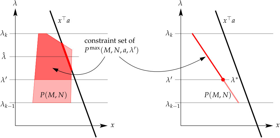 Figure 1
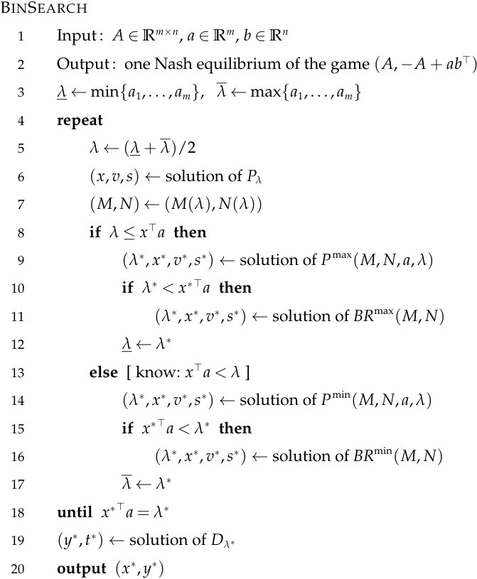 Figure 2
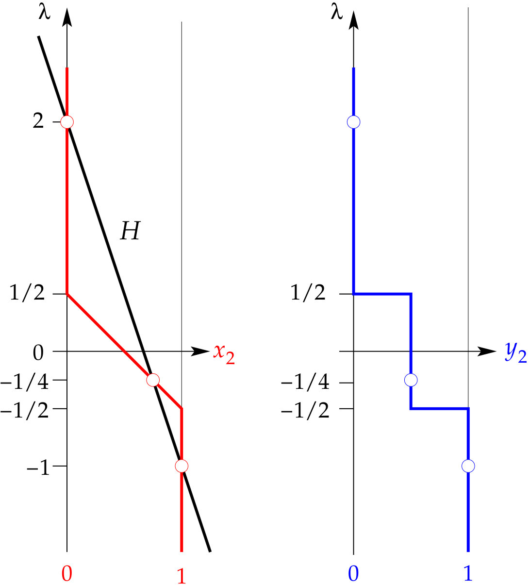 Figure 3
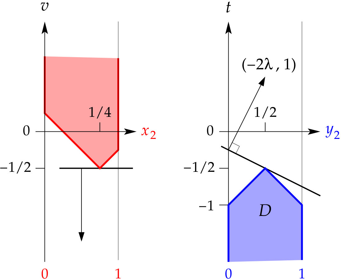 Figure 4
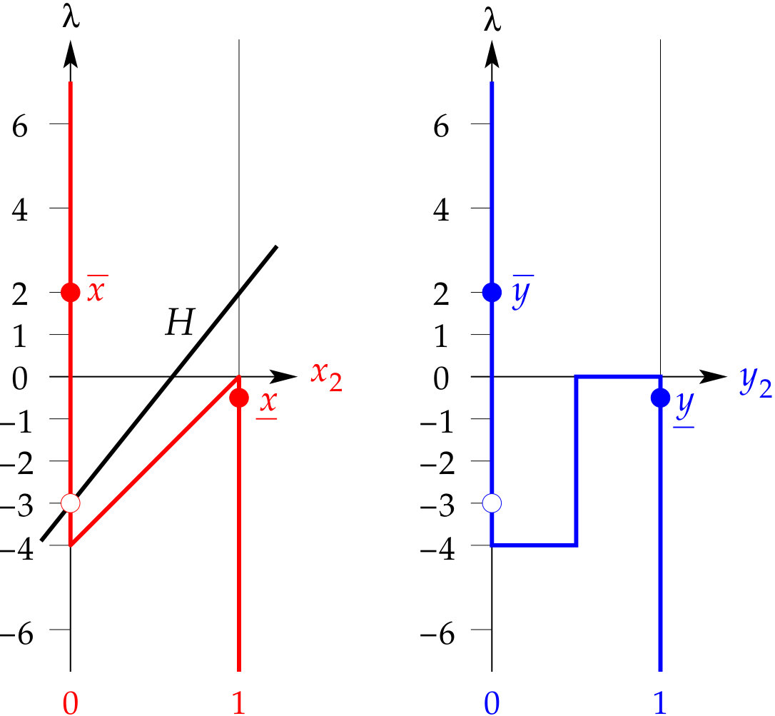 Figure 5
Peer Reviews
No public reviews on file for this paper yet. If you reviewed it on a platform where reviews are public (OpenReview, ICLR, NeurIPS, ICML), you can paste yours below so the community can read it here.
Videos
No videos yet. Explain this paper in a talk, walkthrough, or lecture? Add one.
Fast Algorithms for Rank-1 Bimatrix Games
Bharat Adsullabel=e1][email protected]=u1 [[
Jugal Garglabel=e2][email protected]=u2 [[
url]www.jugal.ise.illinois.edu
Ruta Mehtalabel=e3][email protected]=u3 [[
url]www.rutamehta.cs.illinois.edu
Milind Sohonilabel=e4][email protected]=u4 [[
Bernhard von Stengel label=e5][email protected] label=u5 [[
url]www.maths.lse.ac.uk/Personal/stengel
Department of Computer Science and Engineering, Indian Institute of Technology Bombay, Powai, Mumbai 400 076, India,
University of Illinois at Urbana-Champaign, Urbana, IL 61801, USA,
Department of Mathematics, London School of Economics, London WC2A 2AE, United Kingdom, ;
Abstract
The rank of a bimatrix game is the matrix rank of the sum of the two payoff matrices. This paper comprehensively analyzes games of rank one, and shows the following: (1) For a game of rank , the set of its Nash equilibria is the intersection of a generically one-dimensional set of equilibria of parameterized games of rank with a hyperplane. (2) One equilibrium of a rank-1 game can be found in polynomial time. (3) All equilibria of a rank-1 game can be found by following a piecewise linear path. In contrast, such a path-following method finds only one equilibrium of a bimatrix game. (4) The number of equilibria of a rank-1 game may be exponential. (5) There is a homeomorphism between the space of bimatrix games and their equilibrium correspondence that preserves rank. It is a variation of the homeomorphism used for the concept of strategic stability of an equilibrium component.
bimatrix game,
Nash equilibrium,
rank-1 game,
polynomial-time algorithm,
homeomorphism,
keywords:
\startlocaldefs\endlocaldefs
1 Introduction
Non-cooperative games are basic economic models. The main concept to analyze them is Nash equilibrium, which recommends to each player a (typically randomized) strategy that is optimal for that player if the other players follow their recommendations. In order to give such a recommendation, a Nash equilibrium must be found by some method (including any adjustment process). For larger games this requires computer algorithms. We consider bimatrix games, which are two-player games in strategic form. The algorithm by Lemke and Howson (1964) finds one equilibrium of a bimatrix game. Finding all equilibria is feasible only for small games because of the exponential number of mixed strategies that typically need to be checked for the equilibrium property (Avis, Rosenberg, Savani, and von Stengel, 2010).
Kannan and Theobald (2010) introduced a hierarchy of bimatrix games based on the matrix rank of the sum of the two payoff matrices. Games of rank 0 are zero-sum games, which can be solved by linear programming. This paper comprehensively studies games of rank 1. Rank-1 games are economically more interesting than zero-sum games, by allowing a “multiplicative” interaction in addition to an arbitrary zero-sum component (discussed further in Section 10). We will show that, like general bimatrix games, they can have exponentially many disjoint equilibria. On the other hand, as our main results show, they are computationally tractable: One equilibrium of a rank-1 game can be found fast (in polynomial time), and finding all equilibria takes comparable time to finding a single equilibrium of a general bimatrix game. Large rank-1 games are therefore attractive as detailed models of interaction, on a similar scale to, but more general than, zero-sum games. Rank-1 bimatrix games and their computational analysis should therefore become a new tool in economic modeling.
The computational complexity (required running time) of computing a Nash equilibrium of a game has received substantial interest in the last two decades. A computational problem is considered tractable if it can be solved in polynomial time. Savani and von Stengel (2006) showed that the algorithm by Lemke and Howson (1964) may have exponential running time. (Their examples require carefully constructed matrices, comparable to linear programs where the simplex algorithm, which otherwise works well in practice, has exponential running time, see Klee and Minty, 1972.) The path-following Lemke–Howson algorithm implies that finding an equilibrium of a bimatrix game belongs to the complexity class PPAD defined by Papadimitriou (1994). PPAD describes certain computational problems where the existence of a solution is known, and the problem is to find one explicit solution. (In contrast, the better known complexity class NP applies to decision problems, which are problems that have a “yes” or “no” answer.) Other problems in PPAD include the computation of an approximate Brouwer fixed point, related problems in economics such as market equilibria (Vazirani and Yannakakis, 2011), and the computation of an approximate Nash equilibrium of a game with many players. (In games with three or more players, unlike in two-player games, the mixed strategy probabilities in a Nash equilibrium may be irrational numbers. A suitable concept for such games is approximate Nash equilibrium, and finding an exact Nash equilibrium is an even harder computational problem, see Etessami and Yannakakis, 2010.) A celebrated result is that all problems in PPAD can be reduced to finding a Nash equilibrium in a bimatrix game, which makes this problem “PPAD-complete” (Chen and Deng, 2006; Chen, Deng, and Teng, 2009; Daskalakis, Goldberg, and Papadimitriou, 2009). No polynomial-time algorithm for finding a Nash equilibrium of a general bimatrix game is known.
Kannan and Theobald (2010) describe an algorithm to find -approximate Nash equilibria in games of fixed rank, with running time that is polynomial in and the input length, but exponential in the rank. In the present paper, we prove that an exact Nash equilibrium of a rank-1 game can be found in polynomial time. However, we also show that a rank-1 game may have exponentially many equilibria. Moreover, games of higher fixed rank are PPAD-hard and thus as computationally difficult as general bimatrix games; this has been shown by Mehta (2018) for and is claimed to hold for (Chen and Paparas, 2019). In the context of the “rank” hierarchy, rank-1 games are therefore the most complex type of games that are expected to be computationally tractable.
Section 2 states the notation and preliminary results used in this paper, and compares our approach with the work of Theobald (2009). In Section 3, we show that the set of equilibria of a game of rank is the intersection of a hyperplane with a set of equilibria of parameterized games of rank . When , these are parameterized zero-sum games whose equilibria are the solutions to a parameterized linear program (LP). In order to deal with possibly degenerate games which are awkward to handle with pivoting methods, we recall relevant results from Adler and Monteiro (1992) in Section 4. The intersection with the hyperplane gives rise to a polynomial-time binary search for one equilibrium of a rank-1 game, explained in Section 5. In Section 6, we describe completely the set of all Nash equilibria of a rank-1 game, and outline a corresponding equilibrium enumeration method.
Section 7 describes an example (which may be useful to consult in between) that illustrates our main results, and a second example that shows that binary search fails in general for games of rank 2 or higher. A construction of rank-1 games with exponentially many equilibria is shown in Section 8. In Section 9, we describe a variant of the structure theorem of Kohlberg and Mertens (1986), which is important for the concept of strategic stability of an equilibrium component. We introduce a new homeomorphism between the space of bimatrix games and its equilibrium correspondence. This homeomorphism preserves the sum of the payoff matrices, and hence the rank of the games. In the concluding Section 10, we present a tentative example of an economic model based on rank-1 games, and note some open questions.
A preliminary version of our work was published in STOC 2011 (Adsul, Garg, Mehta, and Sohoni, 2011), and the result of Section 8 in von Stengel (2012). The mathematical development in the present paper is almost entirely new in all parts.
2 Bimatrix games and best responses
In this section we state our notation for bimatrix games and recall the “complementarity” characterization of Nash equilibria in terms of suitable polyhedra. We also briefly compare our approach with Theobald (2009).
We use the following notation. The transpose of a matrix is written . All vectors are column vectors, so if then is an matrix and is the corresponding row vector in . In matrix products, scalars are treated like matrices. Let and be vectors with all components equal to 0 and 1, respectively, their dimension depending on the context. Inequalities like hold for all components. The components of a vector are .
For and , a hyperplane is of the form , and a halfspace of the form . A polyhedron is an intersection of finitely many halfspaces, and called a polytope if it is bounded. A face of a polyhedron is of the form where . It can be shown that any face of can be obtained by turning some of the inequalities that define into equalities (Schrijver, 1986, Section 8.3). If a face of consists of a single point, it is called a vertex of . If for sets , then for some is called the projection of on , also written as .
A bimatrix game is a pair of matrices with rows as pure strategies of player 1 and columns as pure strategies of player 2. The players simultaneously choose their pure strategies, with the corresponding entry of as payoff to player 1 and of to player 2. The sets and of mixed (that is, randomized) strategies of player 1 and player 2 are given by
[TABLE]
For the mixed strategy pair , the expected payoffs to the two players are and , respectively. A best response of player 1 against maximizes his expected payoff , and a best response of player 2 against maximizes her expected payoff . A Nash equilibrium (NE) is a pair of mutual best responses.
Consider mixed strategies and . If is a best response to , then its expected payoff is clearly at least the payoff for any pure strategy of player 1. Moreover, is a best response to if and only if any pure strategy in the support of (that is, where ) is a pure best response to (Nash, 1951). The following lemma, due to Mangasarian (1964), states this “best-response condition” in terms of suitable polyhedra.
Lemma 1**.**
Let be an bimatrix game. Consider the polyhedra
[TABLE]
Let . Then is a best response to if and only if and for all rows
[TABLE]
and is a best response to if and only if and for all columns
[TABLE]
If both conditions hold, then and are the unique payoffs to player 1 and 2 in the Nash equilibrium .
A bimatrix game is degenerate if there is a mixed strategy that has more pure best responses than the size of its support (von Stengel, 2002). A degenerate game may have infinite sets of equilibria. They can be described by suitable faces of of and , as explained further in Section 6. Our analysis applies to general games that may be degenerate.
The object of study of our paper are bimatrix games of fixed rank, introduced by Kannan and Theobald (2010). They generalize zero-sum games, which are games of rank zero.
Definition 2**.**
The rank of a bimatrix game is the matrix rank of .
For comparison of our approach with Theobald (2009), we consider a quadratic program, due to Mangasarian and Stone (1964), that captures the NE of .
Lemma 3**.**
The strategy pair is a Nash equilibrium of if and only if it is a solution to
[TABLE]
The optimum value of is zero, with and .
Proof.
Consider any solution to (5). Then is at least the best-response payoff of player 2 against because , and is at least the best-response payoff of player 1 against because . Hence, . Furthermore, (3) and (4) imply that is zero if and only if is a NE, in which case and .
∎
The quadratic program (5) shows the importance of the rank of the matrix . For zero-sum games, the rank of is zero and (5) is a linear program, a well-known fact (Dantzig, 1963). For a rank-1 game with , the bilinear term in the objective function becomes the product of two linear terms. The resulting optimization problem is called a linear multiplicative program. Solving a general linear multiplicative program is NP-hard (Matsui, 1996).
Consider a rank-1 game where . Similar to parametric simplex methods for solving linear multiplicative programs (Konno, Yajima, and Matsui, 1991), Theobald (2009) describes an algorithm to enumerate all equilibria of . For a real parameter , he considers the parameterized LP
[TABLE]
In any solution to (6), . Hence, by Lemma 3, any optimal solution to (6) is an equilibrium of if and only its optimum is zero. Moreover, implies that is a convex combination of the components of , so that one can restrict to the interval . By partitioning this interval into segments where (6) uses the same basic variables, Theobald (2009) obtains an enumeration of all NE of .
Our approach is somewhat similar, with a parameter and the equality . However, we consider a different LP which is parameterized by and involves only the payoff matrix and the vector used in . That LP, given in (19) below, has as primal and as dual variables, whereas in (6) both and are primal with less closely related constraints. We consider the hyperplane defined by separately from the parameterized LP. The intersection of the hyperplane with the solutions to the parameterized LP defines the equilibria of the rank-1 game. This structural insight can be used both for finding an exact NE in polynomial time by binary search (see Section 5) and for enumerating all equilibria (see Section 6). As a topic for further research, it may be interesting if this approach can be extended to more general linear multiplicative programs.
3 Rank reduction
The central result of this short section is Theorem 7. It states that the set of Nash equilibria of a game of rank is the intersection of a set of equilibria of parameterized games of rank with a suitable hyperplane. In subsequent sections, we show how to exploit this property algorithmically when .
The following lemma states the well-known fact that the equilibria of a bimatrix game are unchanged when subtracting a separate constant from each column of the row player’s payoff matrix. Call two games strategically equivalent if they have the same Nash equilibria.
Lemma 4**.**
If , then the game is strategically equivalent to the game .
Proof.
This holds by Lemma 1, because the equilibrium payoff to player 1 in the game changes to in : Clearly, is equivalent to , and is equivalent to .
∎
Lemma 5**.**
An bimatrix game of positive rank can be written as for suitable , , and a game of rank .
Proof.
An matrix is of rank at most if and only if it can be written as the sum of rank-1 matrices, that is, as for suitable and for . This is easily seen by writing the th column of the matrix as and letting (see also Wardlaw (2005)). Suppose is of rank , with and therefore . Let and , , so that ; obviously, is of rank .
∎
The following is a simple but central lemma.
Lemma 6**.**
Let , , , , , . The following are equivalent:
(a) is an equilibrium of ,
(b) is an equilibrium of and ,
(c) is an equilibrium of and .
Proof.
The equivalence of (a) and (b) holds because the players get in both games the same expected payoffs for their pure strategies: this is immediate for player 1, and if , then the column payoffs are given by
[TABLE]
The games in (b) and (c) are strategically equivalent by Lemma 4.
∎
Consider a game of positive rank where so that is a game of rank according to Lemma 5. Then the game in Lemma 6(c) has the same sum of its payoff matrices and hence also rank , for any choice of the parameter . Let be the set of Nash equilibria together with of these parameterized games,
[TABLE]
where by Lemma 6(b)
[TABLE]
These considerations imply the following main result of this section.
Theorem 7**.**
Given a bimatrix game , its set of Nash equilibria is exactly the projection on of the intersection of and the hyperplane defined by
[TABLE]
Theorem 7 asserts that for any rank- game of the form , every Nash equilibrium of the game is captured by the set in (8) of games of rank which are parameterized by , intersected with the hyperplane in (10). Can this rank reduction be leveraged to get an efficient algorithm to find a Nash equilibrium for a game of arbitrary constant rank? As will be discussed in Section 7, this does not work in general. However, it does work for rank-1 games.
4 Parameterized linear programs
Our aim is to describe the equilibria of rank-1 games using the rank reduction of the previous section. For this, we consider the set in (9) for ,
[TABLE]
where by (8)
[TABLE]
which is the set of equilibria of zero-sum games parameterized by . These correspond to the solutions of a parameterized linear program (LP). In this section, we review the structure of such parameterized LPs with a particular view towards nongeneric cases and polynomial-time algorithms as studied by Adler and Monteiro (1992). In essence, such parameterized LPs have finitely many special values of the parameter called breakpoints. These separate the set into a connected sequence of polyhedral segments (which generically are line segments). They are described in Theorem 16 in the next section, where we will present a polynomial-time algorithm for finding one equilibrium of a rank-1 game. In the subsequent section we present another algorithm for finding all equilibria.
We assume familiarity with notions of linear programming such as LP duality and complementary slackness; see, for example, Schrijver (1986). The following well-known lemma (Dantzig, 1963, p. 286) states that the equilibria of a zero-sum game are the primal and dual solutions to an LP.
Lemma 8**.**
Consider an zero-sum game . In any equilibrium of this game, is a minmax strategy of player 2, which is a solution to the LP with variables in and in :
[TABLE]
and is a maxmin strategy of player 1, which is a solution to the dual LP to . For the optimal value of in , the maxmin payoff to player 1 and minmax cost to player 2 and hence value of the game is .
Proof.
The dual LP to (13) has variables and and states
[TABLE]
Both LPs are feasible (with sufficiently small and large ). Let be an optimal solution to (13) and to (14). Then by LP duality, and (13) and (14) state , that is, player 2 pays no more than for any row, and , that is, player 1 gets at least in every column, where which is therefore the value of the game.
With the dual constraints written as , the complementary slackness conditions between the primal and the dual are exactly the Nash equilibrium conditions (3) and (4) of Lemma 1 (except for the changed sign of so that we do not have to write in (14) as and ). Hence, is a Nash equilibrium.
∎
Applied to in (12), the LP (13) in Lemma 8 says:
[TABLE]
In (15), the matrix is parameterized. The substitution gives the equivalent LP where only the objective function is parameterized:
[TABLE]
This is a standard parameterized linear programming problem. We stay close to the notation of Adler and Monteiro (1992) who consider a primal LP with minimization subject to equality constraints, variables , and a parameterized right hand side, of which (16) is the dual, a maximization problem subject to inequalities, with variables , and a parameterized objective function. We write (16) as
[TABLE]
with the fixed polyhedron
[TABLE]
The LP is the dual of the following LP with a parameterized right hand side, where we use slack variables to express the inequality as an equality, in line with Adler and Monteiro (1992):
[TABLE]
For optimal solutions to and to we have . The next lemma (essentially a corollary to Lemma 6 and Lemma 8) states that and can be interpreted as the player’s payoffs for the games in Lemma 6(a) and (b), and asserts that are uniquely determined by (that is, a point on ).
Lemma 9**.**
Let . Then is an equilibrium of the game if and only if is an optimal solution to in for some which is uniquely determined by , and is an optimal solution to in for some and which are uniquely determined by and . The equilibrium payoffs are to player 1 and to player 2. If , these are also the payoffs in the game , and is an equilibrium of that game.
Proof.
By Lemma 6 with , the game has the same equilibria and, by (7), payoffs as the game if . Consider any optimal solutions to and to . Then states for each row of the inequality . Complementary slackness, equivalent to LP optimality, states that whenever . This is the equilibrium condition in (3) that states that is a best response to . Because it holds for at least one , it uniquely determines , which is the equilibrium payoff to player 1 in the above games.
Similarly, the constraint in (19) means that is determined by , and states for all , or equivalently . Complementary slackness, equivalent to LP optimality, states that this inequality is tight whenever . This is the condition (4) that states that is a best response to in the game , and it uniquely determines as the equilibrium payoff to player 2.
∎
Primal-dual pairs of LPs with a parameter have been studied since Gass and Saaty (1955). The next result is well known, which we show following Jansen, De Jong, Roos, and Terlaky (1997).
Lemma 10**.**
For , let be the optimum value of and hence of . Then is the pointwise maximum of a finite number of affine functions on and therefore piecewise linear and convex.
Proof.
The optimum of exists for any and is taken at a vertex of the polyhedron in (18). Let be the set of vertices of , which is finite. Hence,
[TABLE]
where for each of the finitely many in the function is affine. Hence, is the pointwise maximum of a finite number of affine functions as claimed. The epigraph of given by is the intersection of the convex epigraphs of these affine functions, so is convex and is a convex function.
∎
By (20), the function is the “upper envelope” of the affine functions defined by the vertices of . A breakpoint is any so that has different left and right derivatives when approaches from below or above, denoted by and , respectively.
For any LP , say, let be the face of the domain of where its optimum is attained. For any we denote by , that is,
[TABLE]
Then the left and right derivatives of at are characterized as follows (obvious from (20), also Prop. 2.4 of Adler and Monteiro (1992)):
[TABLE]
which are the optima of the two LPs
[TABLE]
That is, is a breakpoint if and only if . Clearly, in that case there are at least two vertices and of that define two different affine functions and that meet at to define the maximum in (20). These are also vertices of , which is then a higher-dimensional face (such as an edge) of . The following central observation shows that the breakpoints give all the information about the optimal faces of for any between these breakpoints.
Theorem 11**.**
(Adler and Monteiro, 1992, Theorem 4.1) ** Let be the breakpoints, in increasing order, for the parameterized LPs and , and let and . For , consider any . Then for , and for .
For finding the solutions to as a function of , the nondegenerate case is straightforward, where is a vertex of unless is a breakpoint, in which case is an edge of . Then these vertices uniquely describe the pieces of the piecewise linear function , and can be traversed by a parameterized simplex algorithm Gass and Saaty (1955). An example is shown in the right diagram of Figure 4 below with the constraints (44) for in , with the additional constraints to represent , and objective function given by . The three linear parts of are
[TABLE]
which correspond to the optimal vertices of given by , , and . The two breakpoints are and which correspond to the two edges of .
In the degenerate case, one typically does not get polynomial-time algorithms by considering vertices and corresponding basic solutions to the LP as in a parameterized simplex algorithm. Instead of partitioning the variables of into basic and nonbasic variables, Adler and Monteiro (1992) consider “optimal partitions”; we use here only the partition part that replaces the nonbasic variables, which we denote by in (26) below (called in Adler and Monteiro (1992)). This is the set of variables of the dual LP that may be strictly positive in an optimal solution, which represent the “true inequalities” of .
Definition 12**.**
For some suppose that the constraints in
[TABLE]
are feasible. Then any row of so that for some feasible is called a true inequality of .
If there are solutions and to (25) so that and then both inequalities are true for , so there is a unique largest set of true inequalities with some feasible solution where all these strict inequalities hold simultaneously. These define the relative interior of the polyhedron defined by (25).
Let and . Let be the set of true inequalities of the optimal face of in , that is,
[TABLE]
Any non-true inequality of is always tight, that is, if and if . It can be shown that for such and there are optimal solutions to where and , so these are the true inequalities of . This is also known as “strict complementary slackness” (Schrijver, 1986, Section 7.9). Consider the polyhedron of the constraints for in (19) where is allowed to vary,
[TABLE]
The following lemma considers the face of defined by the equations for and for , which are necessary and sufficient for a feasible solution to to be optimal. This is immediate from the standard complementary slackness condition.
Lemma 13**.**
Let and . For and , with and , define
[TABLE]
Then any feasible solution to is optimal if and only if .
Crucially, according to Theorem 11, for any in an open interval (for ) the optimal face is constant in . Hence, for all the true inequalities of are equal to some fixed , and for the points in the value of can be any real in the closed interval . Namely, with the LPs
[TABLE]
the following holds.
Lemma 14**.**
Consider and for as in Theorem 11. Let and (which do not depend on the choice of ). Then for ,
*(a) *the breakpoint is the optimum of the LP and of the LP ;
*(b) *if then .
Proof.
See Adler and Monteiro (1992), p. 171 for (a), and Theorem 3.1(a) and Lemma 3.1(b) for (b).
∎
Lemma 14(a) implies that for any in the open interval , for , the endpoints of the closed interval are given by the minimum and maximum of for where and . Lemma 14(b) and Lemma 13 imply that if is itself a breakpoint, then .
As we will describe in detail in the next section, Theorem 11 and Lemma 14 lead to a description of the set of optimal solutions to and for all with the help of the breakpoints in the form of polyhedral segments (which are lines in the nondegenerate case). Any solution to is optimal if and only if belongs to , which is a face of , and any solution to is optimal if and only if it belongs to , which is a face of . For between two breakpoints, these faces do not change (but typically varies with ), and their Cartesian product defines of the segments. If is equal to a breakpoint, the set is a subset of the two adjoining faces for near , whereas is a superset of the adjoining faces , as described in Theorem 11. This defines the other segments. Using this we will give a precise description of the set in Theorem 16 below.
Adler and Monteiro (1992) describe how to generate the breakpoints of in polynomial time per breakpoint, with a polynomial-time algorithm applied to the LPs (17), (23), (29), which we will adapt to our purpose. (However, the number of breakpoints may be exponential, see Murty (1980).) The true inequalities in Definition 12 can also be found with an LP, according to the following lemma (Prop. 4.1 of Adler and Monteiro (1992)), due to Freund, Roundy, and Todd (1985); for an alternative polynomial-time algorithm see Mehrotra and Ye (1993).
Lemma 15**.**
For and the constraints consider the LP
[TABLE]
Then is feasible if and only if is feasible and bounded, and any optimal solution to satisfies (and otherwise) if and only if is a true inequality of . For such an optimal solution to , is a solution to where for all true inequalities .
Proof.
If the LP is feasible then it is also bounded because . Let be the set of true inequalities of (25), that is, for for some with . Choose so that for all . Then for . Hence, and defined by if , and otherwise, give a feasible solution to the LP (30). This solution is also optimal because any solution to (30) where would give a solution to (25) with and thus , so for any feasible solution to (30) we have whenever . This proves the claim.
∎
5 Finding one equilibrium of a rank-1 game by binary search
We use the results of the previous section to present a polynomial-time algorithm for finding one equilibrium of a rank-1 game , using binary search for a suitable value of the parameter in Theorem 7. The search maintains a pair of successively closer parameter values and corresponding equilibria of the game that are on opposite sides of the hyperplane in (10). Generically, the set in (11) is a piecewise linear path which has to intersect between these two parameter values. In general, the segments of that “path” are products of certain faces of the polyhedra in (17) and in (27) described in Theorem 11 and Lemma 14 using the breakpoints of the LPs and .
We give a complete description of in terms of these faces of and , which we project to (for the possible values of ) and . Namely, consider and for as in Theorem 11. For , define
[TABLE]
Note that for any (for any ) the components and are uniquely determined by by Lemma 9. Similarly, let
[TABLE]
where again in is uniquely determined by . Recall that the choice of does not matter for the definitions of and . The polyhedra for (which for and are infinite, otherwise bounded) represent of the segments that constitute between any two breakpoints and . They are successively connected by further segments, which are polytopes that correspond to the breakpoints themselves. These are for defined by
[TABLE]
and
[TABLE]
Theorem 16**.**
The set in is given by
[TABLE]
where for we have
[TABLE]
and
[TABLE]
Proof.
This follows from Lemma 9, Lemma 13, and Theorem 11. By Theorem 11, is the optimal face of which is a subset of . Hence, , and similarly , which implies (36). In addition, we have and and thus because of the additional tight constraints in . Similarly, . This shows (37).
∎
The preceding characterization of is used in the following lemma.
Lemma 17**.**
Let and and so that for in
[TABLE]
Then for some with .
Proof.
Consider the largest so that and there are with and , which exists since fulfills this property and is closed by Theorem 16.
If then both and belong to the same set or which is convex, where since and we have for a suitable convex combination of and , and , as claimed.
Hence, we can assume . Suppose is a breakpoint , so that . Consider and where by maximality of . By (37), we have and hence . Because and , a suitable convex combination of and belongs to and fulfills as claimed (in fact, does by maximality of ). If is not a breakpoint, we directly have for some and can choose with and apply the same argument.
∎
The binary search algorithm will maintain (38) as an invariant while halving the length of the interval in each iteration.
Lemma 17 ensures that the interval contains some with and (which is not true when applied to games of higher rank, as shown in the example in Figure 5 below). Let and let be the strategy of player 1 in an equilibrium of the game , which is found as a solution to . If , it is natural to proceed with set to (written as ), otherwise with . The binary search should terminate once and are in the same interval between two breakpoints, with the desired equilibrium found in .
However, this straightforward approach has the following problems:
(i) the search may converge to an equilibrium with where is a breakpoint , so that and are always in different intervals and and the described termination condition fails;
(ii) the number of digits to describe and may pile up, which slows down solving .
We address these problems as follows. First, we identify with , the face of that contains . We then check if that face contains some with . Depending on whether or , this is achieved by one of the following variations of the LPs in (29) (these variations will also be used for the enumeration of all equilibria in Section 6):
[TABLE]
Figure 1 illustrates where , and is between two breakpoints and (but could also be a breakpoint itself), so that is projected to . Here the optimal solution to is not unique, but always fulfills . Moreover, and intersect. In the left diagram in Figure 1, is not just a line segment but a higher-dimensional polytope. It contains some and with , for example for , but not for nor . In the right diagram of Figure 1, we always have , and attains its optimum at because for the corresponding , shown as a dot, is least negative. Here, the solution would be more useful for proceeding because it is the next breakpoint. We will introduce an extra computation step to achieve this, as we discuss further below.
The next lemma states that the appropriate LP in (39) identifies if there is an equilibrium of the game with for some between and the next breakpoint .
Lemma 18**.**
Let be a breakpoint of and as in Theorem 11, . Let , let be an optimal solution to , and let as in .
*(a) *Suppose and . Let be an optimal solution to . Then , and the game has an equilibrium with for some if and only if this holds for and .
*(b) *Suppose and . Let be an optimal solution to . Then , and the game has an equilibrium with for some if and only if this holds for and .
Proof.
We prove (a), where (b) is entirely analogous. By Lemma 13, is feasible for . Clearly , and Lemma 14 implies . Because for any feasible solution , the objective function is nonpositive, and zero and hence optimal if and only if , in which case is part of the described equilibrium .
∎
We now describe the BinSearch algorithm in Figure 2, where we will return to the LPs in (39). The conditions and mean that is a convex combination of the components of , so that we can initialize and as their minimum and maximum in line 3 of the algorithm. The main loop of the algorithm is between lines 4 and 18. The candidate value for (called in the above explanations) is the midpoint between and in line 5. Line 6 computes some optimal solution of the LP in (19), where the dual LP in (17) is typically solved alongside . The optimum of and determines the optimal face of in (21). The true inequalities of in line 7 are determined according to (26), for example with the help of the LP in Lemma 15.
Lines 8 to 12, and symmetrically 13 to 17, use the LPs in (39). In order to match the notation in the discussion before Lemma 18, let . Consider the case , handled in lines 8 to 12. Line 9 invokes the LP . By Lemma 18, the optimum to this LP will find the desired equilibrium with if there is one for some up to the next breakpoint , that is, for . Suppose this is not the case, that is, and the optimum of is negative. By Lemma 18, in this case the next breakpoint does not define an equilibrium, so that problem (i) above does not occur. However, as shown in the right diagram in Figure 1, this may result in . We could simply continue with as in line 12, but if this increases the description size of which we would like to keep bounded to avoid problem (ii) (the description size of probably increases only by one bit per main iteration, but it is useful to keep it independent of the number of iterations both for the computation and for the analysis). In line 10, the condition recognizes that the current segment of contains no equilibrium, and then in line 11 computes as the next breakpoint according to Lemma 14(a); the LP in line 11 can be solved by starting from the current solution to . The left diagram in Figure 1 shows that we cannot simply replace the objective function of by : While this would compute the next breakpoint , it may overlook that the current segment of defined by intersects the hyperplane ; this could possibly miss the equilibrium altogether, for example if as shown in the diagram (in particular if still has its initial value, which is not checked in the algorithm as to whether it produces an equilibrium).
In summary: lines 8 to 11 find and so that either (a) , or (b) and is a breakpoint and , which implies . The next value of is set to in line 12. In case (a), the loop terminates in line 18. In case (b), the loop continues, and in the next iteration the difference has shrunk by at least one half. The analogous statements hold for lines 13–17. The following theorem states the correctness and polynomial running time of the algorithm.
Theorem 19**.**
Algorithm BinSearch finds one equilibrium of the rank-1 game . Assume that the entries of are rational numbers with combined bit length , and that LPs are solved with polynomial-time solvers that return extreme LP solutions obtained from linear equations derived from . Then BinSearch runs in polynomial time in .
Proof.
During the main loop, the invariant (38) is preserved, and the length of the interval shrinks by at least a factor of two per iteration. By Lemma 17, a solution with and is guaranteed to exist. The termination condition in line 18 holds once reaches a segment of that intersects , which is identified with one of the LPs in line 9 or 14 by Lemma 18. Because the length of the search interval shrinks by at least half in each iteration, the search interval eventually contains at most one breakpoint . If there is no breakpoint in , then for . Hence, a solution to or to determines an equilibrium to by Lemma 18 and Lemma 6. This holds also if there is a single breakpoint in . Hence, as claimed, the algorithm computes an equilibrium of .
The number of overall iterations is polynomial for the following reason. Any breakpoint is part of a vertex of by Lemma 14(a). This vertex is a solution to a linear system of equations where each component (such as ) is a fraction with an integer determinant obtained from in the denominator (which has a polynomial of bits), and distinct fractions for different breakpoints . Hence, any two breakpoints have minimum distance for some polynomial (see also (Schrijver, 1986, Section 10.2)). Therefore, there will be at most binary search iterations until the search interval contains at most one breakpoint and the search terminates.
Each iteration of the algorithm solves three or four LPs. The first is in line 6. Using the optimum of that LP, in line 7 the true inequalities in (26) of in (21) are found with another LP as in Lemma 15. The third LP is either in line 9 or in line 14. The fourth LP is either or in line 11 or 16, respectively (which just relaxes the extra constraints of the previous LP in (39) and has a different objective function). In all cases, the output is described in terms of and found in polynomial time in the bit size , and itself has polynomial bit size (Schrijver, 1986, Corollary 10.2a(iii)). In the next iteration, determines with the constant arithmetic expression in line 5 the next parameter for in line 6 and for in line 7 so that the bit size of remains polynomial in . Hence, each main iteration takes polynomial time, and the overall running time is polynomial.
∎
In practice, as observed in (Adler and Monteiro, 1992, Section 5), in the nondegenerate case the segments of are line segments. Then the LP in line 9 or 14 is solved starting from the current solution to in line 6 with a single pivot, and similarly the next LP in line 11 or 16.
6 Enumerating all equilibria of a rank-1 game
In this section, we show how to obtain a complete description of all Nash equilibria of a rank-1 game with the help of Theorem 7 and Theorem 16.
A degenerate bimatrix game may have infinite sets of Nash equilibria. They can be described via maximal Nash subsets (Jansen, 1981), called “sub-solutions” by Nash (1951). A Nash subset for is a nonempty product set where and so that every in is an equilibrium of ; in other words, any two equilibrium strategies and are “exchangeable”. Using the “best response polyhedra” and in (2), it can be shown that any maximal Nash subset is a polytope, with as a suitable face of projected to , and as a suitable face of projected to (Avis, Rosenberg, Savani, and von Stengel, 2010). These faces are defined by converting some inequalities in (2) to equations, which have to fulfill the equilibrium conditions (3) and (4). The usual output for “enumerating” all equilibria consists of listing all maximal Nash subsets via the vertices of and . These are vertices of and , respectively (projected to and ) that define the “extreme” Nash equilibria of , with maximal Nash subsets obtained as maximally exchangeable sets of such vertices (Avis, Rosenberg, Savani, and von Stengel, 2010, Prop. 4). Maximal Nash subsets may intersect, in which case their vertex sets intersect. In a nondegenerate game, all maximal Nash subsets are singletons.
For a rank-1 game , its set of Nash equilibria is projected to by Theorem 7, with in (11) and in (10). By (35), is the union of polyhedra, whose nonempty intersections with give almost directly the maximal Nash subsets.
Theorem 20**.**
Let be a rank-1 bimatrix game, and let and for as in Theorem 11. With , , , , let
[TABLE]
Then the maximal Nash subsets of are the sets if , and if and is not equal to or .
Proof.
Each set is the projection of on , and is the projection of on , with and containing the corresponding set of ’s. Hence, by Theorem 16, if then is a Nash subset, and if then is a Nash subset, and the union of these is the set of all equilibria which is the projection of on by Theorem 7. The only question is which of these Nash subsets are inclusion-maximal. By Corollary 3.2 of Adler and Monteiro (1992), where and contain properly, whenever , and whenever , and Lemma 14 implies . So the only possible inclusions are that is a subset of or of . Suppose , that is, and . If this implies then . By Lemma 13, this means is part of an optimal solution to and hence , which shows the proper inclusion because . Similarly, implies . These are the only possible inclusions because if with so that we clearly cannot have , say, where .
This proves the theorem. We also note that the described sets and are defined in terms of the game independently of the parameter . Namely, the condition implies that the polyhedron in (2) for is given by
[TABLE]
so and are projections of certain faces of .
∎
A suitable algorithm that enumerates all Nash equilibria can be adapted from the algorithm by Adler and Monteiro (1992, p. 173) that proceeds from breakpoint to breakpoint using Theorem 11. The corresponding segments of can then be checked for nonempty intersections with , which are then output as maximal Nash subsets if they meet the conditions of Theorem 20.
We give an outline of this algorithm. Suppose is equal to a breakpoint . Then in (34) is the projection of , and in (33) is the projection of by Lemma 14(b) and Lemma 13. If is not empty, its projection to is a maximal Nash subset . Start from some . If then , which is a suitable starting point for the vertex enumeration of the polytope , for example with the program lrs (Avis, 2000). If or then the condition is checked with one of the LPs in (39) by Lemma 18 which then have optimal value zero, with optimum ; then , and is a new starting point to enumerate the vertices of .
The next segment to be tested for its intersection with is in (31) and (32). For that purpose it is not necessary to find some , because by Theorem 11, and the true inequalities of that face are found by Lemma 15, so that one obtains as the projection of . Moreover, we have . If then is also a starting point for the enumeration of the vertices of , which gives the Nash subset (which is, however, not maximal if , see Theorem 20). If then we solve in (39) to find out if intersects the current segment , and similarly if . Finally, the next breakpoint is found as the solution to in (29) by Lemma 14(a).
For initialization and termination of this algorithm, we use that the possible values of can be restricted to with and as minimum and maximum of . The initialization is , which is decided to be a breakpoint or not as described after (23). The constraint is added to the step of finding the next breakpoint, which terminates the algorithm when it is found to hold as equality.
This algorithm, based on Theorem 20, for enumerating all Nash equilibria of a rank-1 game has the following noteworthy features. First, it works for all games (degenerate or not), and its characterization of maximal Nash subsets is simpler than for general bimatrix games (Avis, Rosenberg, Savani, and von Stengel, 2010), and could even be adapted to easily represent these Nash subsets in terms of their inequalities rather than their vertices (which would be of interest if they are high-dimensional). Secondly, the algorithm in effect traverses which is generically a path. Rather than by solving a succession of LPs, it can also be implemented by a variant of the algorithm by Lemke (1965) with the additional linear constraints or , depending on the current sign of . Here, traversing this path gives all Nash equilibria, whereas for general bimatrix games Lemke’s algorithm (as in von Stengel, van den Elzen, and Talman, 2002 or Govindan and Wilson, 2003) only finds one Nash equilibrium.
7 Two examples
In this section, we illustrate the results of the previous sections with an example of a rank-1 game. After that we will give an example that shows that binary search will in general not work for a game of rank 2 or higher, even though Lemma 6 suggests the possibility of finding a Nash equilibrium of such a game via a recursive rank reduction.
Consider the following rank-1 game ,
[TABLE]
where and . This game has the two pure equilibria and , and the mixed equilibrium . By Theorem 7(b), these are the equilibria of the game so that . For , this means .
Figure 3 shows the set in (11) where is an equilibrium of the parameterized game , where
[TABLE]
These equilibria are pure except when , when the unique mixed strategy of player 1 is given by equalizing the column payoffs, , that is, . The white dots indicate the intersection of with the hyperplane in (10), which is defined by the equation , and no constraints on .
Figure 4 shows the domains of the LPs in (19) and in (17) for . Again we show in as and in as . The constraints of are then and , which for are and . The constraints of are
[TABLE]
and the objective function is , with gradient for . For , the optimum of is attained at the vertex of , for at the vertex , and for at the vertex . For and , the optimal face of is an edge of . These are the two breakpoints and in Theorem 11.
Figure 3 also demonstrates the characterization of the path in Theorem 16. The left diagram shows (from left to right) the three pieces , , , each of which happen to intersect . In the central diagram, the vertical parts of the path are , , , and the horizontal parts (for the breakpoints) are and . This corresponds to the following, more elementary game-theoretic explanation. Except when or , player 2’s equilibrium strategy in the game is constant in , which holds because player 1’s payoff matrix does not change with and is chosen so as to make player 1 indifferent between the pure strategies in the support of his equilibrium strategy. When or , the game is degenerate, and player 2’s equilibrium strategies form a line segment, which allows the change of support of her equilibrium strategy .
Our second example shows that the binary search algorithm no longer works for rank- games with . Consider the following game of rank 2:
[TABLE]
where and . Here, is of rank 2 and is of rank 1. The only equilibrium of is the pure equilibrium . The parameterized game has payoff matrices
[TABLE]
It has the following equilibria depending on , which define the set in (9), shown in Figure 5: The pure equilibrium for ; the pure equilibrium for ; the mixed equilibrium for , and two further components with when and with when where the game in (46) is degenerate. These are multiple disjoint equilibrium components for , which cannot happen for a parameterized zero-sum game. As a result, may change non-monotonically along the path , which in general causes a binary search to fail, as we show next.
We describe a suitably adapted binary search method for this example, where instead of solving parameterized LPs we find equilibria of the parameterized game (46) of lower rank. The smallest and largest components of as in line 3 of the BinSearch algorithm are and . For , the only equilibrium of the game in (46) is , but for there are multiple equilibria, where we choose . Then and , so we next consider the midpoint as in line 5 of BinSearch, and compute a new equilibrium of this parameterized game. Suppose this is again , so that because the assignment takes place for the binary search to continue. This is the situation shown in Figure 5. At this point, the method will no longer succeed in finding a suitable value of because the search interval no longer contains the only possible value for , namely . The problem is that in that interval, the set consists of two disconnected parts where and on opposite sides of the hyperplane , so that no longer intersects with . Hence, even though the values of converge, the corresponding equilibria on the two sides of will not converge.
This example shows that because of the non-monotonicity of along the path , there is no equivalent statement to Lemma 17 that would guarantee that a binary search will succeed.
8 Rank-1 games with exponentially many equilibria
Kannan and Theobald (2010, Open Problem 9) asked if the number of Nash equilibria of a nondegenerate rank-1 game is polynomially bounded. This is not the case, because our next result shows that this number may be exponential.
Theorem 21**.**
Let and let be the bimatrix game with entries of
[TABLE]
for , and . Then is of rank , and is a nondegenerate bimatrix game with many Nash equilibria.
Proof.
By (47), with the components of and defined by and for , so is of rank 1.
Let with support . Consider a row and let . Because is upper triangular, the expected payoff against in row is
[TABLE]
Suppose . If is empty, then , otherwise let and note that for we have , so . Hence, no row outside is a best response to . Similarly, because the game is symmetric, any column that is a best response to in belongs to the support of . This shows that the game is nondegenerate. Moreover, if is an equilibrium of , then and have equal supports.
For any nonempty subset of , we construct a mixed strategy with support so that is an equilibrium of . This implies that the game has many equilibria, one for each support set . The equilibrium condition holds if for with equilibrium payoff , because then for as shown above. We start with , where , by fixing as some positive constant (e.g., ), which determines . Once is known for all (and for ), we scale and by multiplication with so that becomes a mixed strategy. Assume that and and assume that has been found for all in so that for all in , which is true for . Then, as shown above, for , so is determined by in (48), and . By induction, this determines for all in , and after re-scaling gives the desired equilibrium strategy .
∎
By Theorem 7, the equilibria of a rank-1 game are the intersection of the path in (11) with the hyperplane in (10). The exponential number of Nash equilibria of the game in Theorem 21 shows that has exponentially many line segments. Murty (1980) describes a parameterized LP with such an exponentially long path of length . The payoffs for the game in Theorem 21 have been inspired by Murty’s example, but are not systematically constructed from it, which would be interesting. See von Stengel (2012) for further discussions and related work on the maximal number of Nash equilibria in bimatrix games, such as von Stengel (1999).
9 A rank-preserving structure theorem
Nash equilibria of games are in general not unique, which has led to a large literature on equilibrium refinements (van Damme, 1991) that impose additional conditions on equilibria, such as stability against small changes in the game parameters, as proposed in the seminal paper by Kohlberg and Mertens (1986) (KM). They showed that stability has to apply to equilibrium components, that is, maximal sets of equilibria that are topologically connected (which for bimatrix games are unions of intersecting maximal Nash subsets, see Section 6). That is, an equilibrium component is stable if every perturbed game has an equilibrium near that component (although possibly in different positions depending on the perturbation, which is why any single equilibrium may fail to be stable). KM proved the existence of stable equilibrium components with the help of a structure theorem (Kohlberg and Mertens, 1986, Theorem 1) which states that the equilibrium correspondence over the set of strategic-form games with a given number of players and numbers of strategies is homeomorphic to itself.
In this section, we present in Theorem 23 a similar structure theorem with a new homeomorphism for bimatrix games that preserves rank. In analogy to Kohlberg and Mertens (1986, Appendix B), one consequence of this new structure theorem is the existence of an equilibrium component in a game that is stable with respect to small perturbations that preserve the sum of the payoff matrices. This is not interesting for zero-sum games which always have only one component, but it is for games of higher rank and applies, for example, to perturbations of the matrix in a rank-1 game given as . Furthermore, a number of equilibrium-finding algorithms can be interpreted as following a path on the equilibrium correspondence via the KM homeomorphism and suitable projections (Wilson, 1992; Govindan and Wilson, 2003). As a topic for further research, it may be interesting to study our new homeomorphism in this context, or, similar to Jansen and Vermeulen (2001), the computation of equilibrium components that are stable with respect to small perturbations that preserve the sum of the payoff matrices.
We first recall the KM homeomorphism from Kohlberg and Mertens (1986). Let be the set of bimatrix games and be its equilibrium correspondence,
[TABLE]
To distinguish the dimensions of the all-zero and all-one vectors we write them as and . Let and be the vectors of row and column averages of and ,
[TABLE]
Then and correspond uniquely to pairs and with
[TABLE]
with and as in (50). That is, is parameterized by a “base game” where each row of player 1 and each column of player 2 gets payoff zero when the other player randomizes uniformly (as in , where the factor does not matter), and a pair of vectors in and with in that are added to the rows of and columns of , respectively, to obtain the correct payoffs.
The KM homeomorphism only changes and . It is most easily described by its inverse defined by ,
[TABLE]
That is, has the same “base game” as but different parameters and . The fact that is an equilibrium of implies that is injective (and therefore well-defined), by the following intuition. Because is a best response to , each row of the vector of expected payoffs in the support of has maximal and equal value among all components of , by (3). This condition allows us to re-construct from the sum , which is used in the definition of in (52) and which can be obtained from . Suppose the components of are heights of “poles in the water” of which a certain amount is “above the waterline” depending on the “water level” , where
[TABLE]
so and if then . For any , there is a unique choice of in (53) so that and therefore . By this construction of and , all components of the vector fulfill (a) , and (b) implies , as when and is a best response to . In a similar way, is a best response to and the sum used to define in (52) is special because it allows us first to obtain a vector from , and second to obtain the original and so that and . The following lemma states this construction, which we apply afterwards to define the KM homeomorphism, and will later use again for our new homeomorphism.
Lemma 22**.**
Given and , there are unique , , and so that
[TABLE]
Proof.
For , let , and
[TABLE]
where (and similarly ) is the unique lowest “water level” so that the “heights” of the components of that are “above the waterline” sum up to (at most) one. Then
[TABLE]
and and fulfill (54), and are uniquely determined by the conditions , , and (54).
∎
The KM homeomorphism is then defined as follows.
(a) Let , , and .
(b) Apply Lemma 22 to get so that (54) holds.
(c) Let and , and define and by (51).
Then is continuous because it is defined by continuous linear mappings and (55) and (56) for (b). We show that . We have , and similarly . Then the conditions (54) are equivalent to the best-response conditions (3) and (4), that is, is indeed an equilibrium of . Moreover, and , which shows that the (continuous) function in (52) is indeed the inverse of (so is injective), and also that is surjective, because we can start in (52) from any .
The KM homeomorphism does not operate within a subset of games of fixed rank (for example, the zero-sum games). Our new homeomorphism has this property. Consider a fixed matrix , the set bimatrix games with , and as the equilibrium correspondence in (49) restricted to these games,
[TABLE]
The following theorem states we can restrict to a homeomorphism for any (for example, the all-zero matrix ). Also, is continuous in and therefore a homeomorphism like the KM homeomorphism.
Theorem 23**.**
Let . There is a homeomorphism , , that is, for all .
Proof.
We will use a new parameterization of any matrix in , which corresponds uniquely to a quadruple with , , , and according to
[TABLE]
so that
[TABLE]
It is easy to see that , , , and are uniquely given by , (58), and
[TABLE]
The homeomorphism , uses this parameterization of and only changes the vectors and , and maintains the sum of the payoff matrices, that is, . Like for the KM homeomorphism, we first describe its inverse , which maps in to in . Let and be an equilibrium of . Let be represented as in (58) so that (59) holds, and let
[TABLE]
with and given by
[TABLE]
where and are the linear projections on the hyperplane through the origin with normal vector respectively ,
[TABLE]
which achieves and for any and , as required for a parameterization of the payoff matrix like it is done for in (59). With thus encoded, we let .
The homeomorphism itself is obtained as follows. Let . Similar to (58) we represent by (61) where as in (60)
[TABLE]
which implies
[TABLE]
Given and , we determine , , and by Lemma 22 so that (54) holds. Then, let
[TABLE]
so that and fulfill (59), define by (58), and let . Like before, is defined by linear maps and the continuous operations in (55) and (56) and is therefore continuous.
We show that . Because , we only need to show the equilibrium property. Using (58), , (66), , and the definition of in (63),
[TABLE]
for some which means that for and therefore by (54) the best-response condition (3) holds (which is unaffected by a constant shift), that is, is a best response to . Similarly, using , (66), the definition of in (63), and ,
[TABLE]
for some which means that for and therefore by (54) the best-response condition (4) holds, that is, is a best response to . Hence, is indeed an equilibrium of .
To show that has the inverse described in (61) and (62), note that and in (63) are linear and and . Therefore, for with as in (61), we have by (67) and (68) and because and ,
[TABLE]
that is, has indeed the (continuous) inverse described in (62) and is both injective and surjective. This shows that is indeed a homeomorphsim from to .
∎
10 Conclusions
We conclude with some open questions. Our analysis shows that rank-1 games are computationally easy to analyze: One Nash equilibrium can be found in polynomial time, and enumerating all equilibria can be performed by following a piecewise linear path, similar to finding a single Nash equilibrium of a bimatrix game (which is in general a PPAD-hard problem).
As described in Section 6, the path of solutions to the parameterized LP consists in general of polyhedral segments whose intersections with the hyperplane define the sets of Nash equilibria of the rank-1 game. This set-up suggests the application of smoothed analysis as pioneered by Spielman and Teng (2004) for the “shadow vertex algorithm” for parameterized LPs. This analysis has been subsequently improved and simplified; for recent developments see Dadush and Huiberts (2018). In smoothed analysis, the LP data are perturbed by some moderate Gaussian noise which cancels “pathological” cases that lead to exponential worst-case examples, like the game constructed in Section 8. Applied to our parameterized LP, it would imply that in expectation there is a polynomial number of segments in Theorem 16. If this holds, the number of Nash equilibria is similarly polynomially bounded by Theorem 20 (the Nash subsets are all single equilibria because the perturbed game is generic and therefore nondegenerate with probability one). However, the standard framework of smoothed analysis (as in e.g. Dadush and Huiberts, 2018) assumes that the LP constraints are of the form , which is not the case for the LP (16) that we consider, so combining this with our approach requires a careful study that we leave for future work. For a general bimatrix game, finding one equilibrium is PPAD-hard even under smoothed analysis (Chen, Deng, and Teng, 2009). However, it is not known if a perturbed game may have exponentially long Lemke–Howson paths; the long paths in Savani and von Stengel (2006) do not persist due to exponential size differences in the payoffs.
In Section 8 we described rank-1 games with exponentially many equilibria (also with exponential size differences in the payoffs). This raises the following question: Can all equilibria of a rank-1 game be computed in running time that is polynomial in the size of the input and output? Such an algorithm is called “output efficient”. For example, the algorithm by Adler and Monteiro (1992) that computes all segments of a parameterized LP is output efficient. We have extended this algorithm in Section 6. For general bimatrix games, an output efficient algorithm that finds all Nash equilibria would imply PNP because it is NP-hard to decide if a game has more than one Nash equilibrium (Gilboa and Zemel, 1989). Our binary search algorithm gives no information about the existence of a second equilibrium, so it is conceivable that finding a second Nash equilibrium of a rank-1 game is also NP-hard. The existence of an output efficient algorithm to find all Nash equilibria of a rank-1 game is an open question.
General bimatrix games are computationally difficult, but rank-1 games are computationally easy. One should therefore investigate economic applications of large rank-1 games, also as approximate economic models that can serve as fast-solvable benchmarks. As a possible starting point, we describe here a simple “trade game”, which suggests that rank-1 games are much more versatile and economically interesting than zero-sum games. Let player 1 be a seller of a product who can choose possible quality levels for , and let player 2 be a buyer who can decide on possible quantity levels for that she buys from the seller. A price that is paid from buyer to seller can be chosen arbitrarily for each and . Suppose there are further parameters , , , and so that the payoffs to the players are
[TABLE]
We further assume that , which reflects that high quality is costly to produce for player 1 and beneficial for player 2, with representing the benefits from trade. The additional parameter (increasing with ) is an additional benefit to player 1 for higher amounts of sold quantities, and similarly to player 2 for higher quality. Neither nor affect the players’ best responses and can therefore assumed to be zero. This gives a strategically equivalent game whose sums of payoffs are and therefore of rank one. Because rank-1 games can be analyzed very fast, this “trade game” can be studied for large values of and , and in particular for its possibly many price levels. The concrete economic interpretation of such games and their equilibria remains to be investigated. Bulow and Levin (2006) consider a “multiplication game” which is a matching game between workers and firms where the suitability of a worker for a firm is described by a matrix of rank one. However, it is a game with players, not two players.
Acknowledgments
This material is based upon work supported by the National Science Foundation under Grant No. CRII 1755619 (Jugal Garg) and CAREER award CCF 1750436 (Ruta Mehta).
We thank two anonymous referees of Operations Research for their detailed comments which helped improve the manuscript. Heinrich Nax suggested the “trade game” (70) in Section 10.
The reference list from the paper itself. Each links out to its DOI / PubMed record.
- 1(1)
- 2Adler and Monteiro (1992) Adler, I., and R. D. C. Monteiro (1992), A geometric view of parametric linear programming. Algorithmica , 8(1–6), 161–176.
- 3Adsul, Garg, Mehta, and Sohoni (2011) Adsul, B., J. Garg, R. Mehta, and M. Sohoni (2011), Rank-1 bimatrix games: a homeomorphism and a polynomial time algorithm. In: Proc. 43rd Annual ACM Symposium on Theory of Computing (STOC) , pp. 195–204.
- 4Avis (2000) Avis, D. (2000), lrs: a revised implementation of the reverse search vertex enumeration algorithm. In: Polytopes – Combinatorics and Computation , ed. by G. Kalai and G. Ziegler, pp. 177–198. Birkhäuser Verlag, Basel.
- 5Avis, Rosenberg, Savani, and von Stengel (2010) Avis, D., G. D. Rosenberg, R. Savani, and B. von Stengel (2010), Enumeration of Nash equilibria for two-player games. Economic Theory , 42(1), 9–37.
- 6Bulow and Levin (2006) Bulow, J., and J. Levin (2006), Matching and price competition. American Economic Review , 96(3), 652–668.
- 7Chen and Deng (2006) Chen, X., and X. Deng (2006), Settling the complexity of two-player Nash equilibrium. In: 47th Annual IEEE Symposium on Foundations of Computer Science (FOCS) , pp. 261–272.
- 8Chen, Deng, and Teng (2009) Chen, X., X. Deng, and S.-H. Teng (2009), Settling the complexity of computing two-player Nash equilibria. Journal of the ACM , 56(3), Article 14.