An Anomaly-free Atlas: charting the space of flavour-dependent gauged $U(1)$ extensions of the Standard Model
B. C. Allanach, Joe Davighi, Scott Melville

TL;DR
This paper systematically maps the space of anomaly-free, flavour-dependent gauged U(1) extensions of the Standard Model, providing a comprehensive set of solutions for model building and phenomenology.
Contribution
It introduces a Diophantine analysis method and a computational tool to enumerate all anomaly-free U(1) charge assignments for the Standard Model with right-handed neutrinos.
Findings
Complete solution space for anomaly-free U(1) charges identified
A computational program generating charge assignments up to a maximum absolute charge
Publicly available lists of anomaly-free charge configurations
Abstract
Spontaneously broken, flavour-dependent, gauged extensions of the Standard Model (SM) have many phenomenological uses. We chart the space of solutions to the gauge anomaly cancellation equations in such extensions, for both the SM chiral fermion content and the SM plus (up to) three right-handed neutrinos (SM). Methods from Diophantine analysis allow us to efficiently index the solutions arithmetically, and produce the complete solution space in particular cases. In order to solve the general case, we build a computer program which cycles through possible charge assignments, providing all solutions for charges up to some pre-defined maximum absolute charge. Lists of anomaly-free charge assignments result, which corroborate the results of our Diophantine analysis. We make these lists, which may be queried for further desirable properties, publicly available.…
Click any figure to enlarge with its caption.
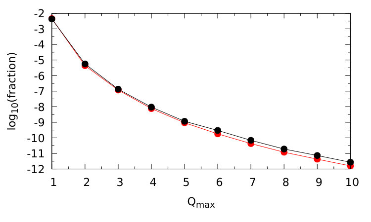 Figure 1
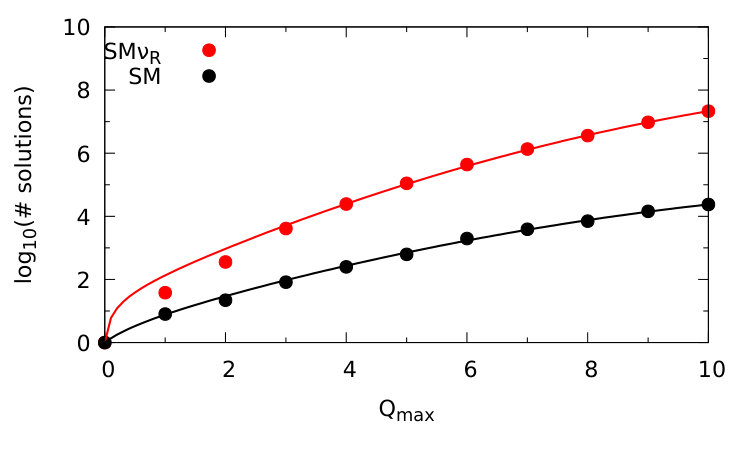 Figure 2
| 1 | 0 | 0 | 0 | 0 | 0 | 0 | 0 | 0 | 0 | 0 | 0 | 0 | 0 | 0 | 0 | 0 | 0 | 0 |
|---|---|---|---|---|---|---|---|---|---|---|---|---|---|---|---|---|---|---|
| 2 | 0 | 0 | 0 | 0 | 0 | 0 | 0 | 0 | 0 | 0 | 0 | 0 | -1 | 0 | 1 | -1 | 0 | 1 |
| 3 | 0 | 0 | 0 | 0 | 0 | 0 | -1 | 0 | 1 | 0 | 0 | 0 | -1 | 0 | 1 | 0 | 0 | 0 |
| 4 | 0 | 0 | 0 | 0 | 0 | 0 | -1 | 0 | 1 | -1 | 0 | 1 | 0 | 0 | 0 | -1 | 0 | 1 |
| 5 | -1 | 0 | 1 | 0 | 0 | 0 | 0 | 0 | 0 | 0 | 0 | 0 | -1 | 0 | 1 | 0 | 0 | 0 |
| 6 | -1 | 0 | 1 | 0 | 0 | 0 | 0 | 0 | 0 | -1 | 0 | 1 | 0 | 0 | 0 | -1 | 0 | 1 |
| 7 | -1 | 0 | 1 | 0 | 0 | 0 | -1 | 0 | 1 | -1 | 0 | 1 | 0 | 0 | 0 | 0 | 0 | 0 |
| 8 | -1 | 0 | 1 | 0 | 0 | 0 | -1 | 0 | 1 | -1 | 0 | 1 | -1 | 0 | 1 | -1 | 0 | 1 |
| Solutions | Symmetry | Quadratics | Cubics | Time/sec | |
|---|---|---|---|---|---|
| 1 | 8 | 8 | 32 | 8 | 0.0 |
| 2 | 22 | 14 | 1861 | 161 | 0.0 |
| 3 | 82 | 32 | 23288 | 1061 | 0.0 |
| 4 | 251 | 56 | 303949 | 7757 | 0.0 |
| 5 | 626 | 114 | 1966248 | 35430 | 0.0 |
| 6 | 1983 | 144 | 11470333 | 143171 | 0.2 |
| 7 | 3902 | 252 | 46471312 | 454767 | 0.6 |
| 8 | 7068 | 336 | 176496916 | 1311965 | 2.2 |
| 9 | 14354 | 492 | 539687692 | 3310802 | 6.7 |
| 10 | 23800 | 582 | 1580566538 | 7795283 | 20 |
| Solutions | Symmetry | Quadratics | Cubics | Time/sec | |
|---|---|---|---|---|---|
| 1 | 38 | 16 | 144 | 38 | 0.0 |
| 2 | 358 | 48 | 31439 | 2829 | 0.0 |
| 3 | 4116 | 154 | 1571716 | 69421 | 0.1 |
| 4 | 24552 | 338 | 34761022 | 932736 | 0.6 |
| 5 | 111152 | 796 | 442549238 | 7993169 | 6.8 |
| 6 | 435305 | 1218 | 3813718154 | 49541883 | 56 |
| 7 | 1358388 | 2332 | 24616693253 | 241368652 | 312 |
| 8 | 3612734 | 3514 | 127878976089 | 978792750 | 1559 |
| 9 | 9587085 | 5648 | 558403872034 | 3432486128 | 6584 |
| 10 | 21546920 | 7540 | 2117256832910 | 10687426240 | 24748 |
| Model | ||||||||||||||||||
|---|---|---|---|---|---|---|---|---|---|---|---|---|---|---|---|---|---|---|
| 0 | 0 | 0 | -1 | 0 | 1 | -1 | 0 | 1 | 0 | 0 | 0 | -1 | 0 | 1 | 0 | 0 | 0 | |
| TFHM | -1 | 0 | 0 | 0 | 0 | 0 | 0 | 0 | 6 | -4 | 0 | 0 | 0 | 0 | 3 | 0 | 0 | 2 |
| -1 | 0 | 0 | 0 | 0 | 3 | 0 | 0 | 3 | -1 | 0 | 0 | 0 | 0 | 3 | -1 | 0 | 0 |
| 1 | -1 | 0 | 0 | 0 | 0 | 2 | 0 | 0 | 4 | -2 | 0 | 0 | 0 | 0 | 3 | 0 | 0 | 0 |
| 2 | -1 | 0 | 0 | -1 | 1 | 2 | 0 | 0 | 4 | -2 | 0 | 0 | 0 | 0 | 3 | 0 | 0 | 0 |
| 3 | -1 | 0 | 0 | -2 | 2 | 2 | 0 | 0 | 4 | -2 | 0 | 0 | 0 | 0 | 3 | 0 | 0 | 0 |
| 4 | -1 | 0 | 0 | -3 | 2 | 3 | 0 | 0 | 4 | -2 | 0 | 0 | 0 | 0 | 3 | 0 | 0 | 0 |
| 5 | -1 | 0 | 0 | -4 | 2 | 4 | 0 | 0 | 4 | -2 | 0 | 0 | 0 | 0 | 3 | 0 | 0 | 0 |
| 6 | -1 | 0 | 0 | -5 | 2 | 5 | 0 | 0 | 4 | -2 | 0 | 0 | 0 | 0 | 3 | 0 | 0 | 0 |
| 7 | -1 | 0 | 0 | -6 | 2 | 6 | 0 | 0 | 4 | -2 | 0 | 0 | 0 | 0 | 3 | 0 | 0 | 0 |
| 8 | -1 | 0 | 0 | -6 | 3 | 5 | -2 | 0 | 6 | -2 | -2 | 2 | -1 | 0 | 4 | 0 | 0 | 0 |
| 9 | -1 | -1 | 1 | 0 | 1 | 1 | -1 | 0 | 5 | -3 | 0 | 1 | 0 | 0 | 3 | 0 | 0 | 0 |
| 10 | -1 | -1 | 1 | -2 | 1 | 3 | -1 | 0 | 5 | -2 | -1 | 1 | -1 | 0 | 4 | 0 | 0 | 0 |
| 11 | -1 | -1 | 2 | -2 | -1 | 3 | -2 | 0 | 2 | -1 | -1 | 2 | -1 | 0 | 1 | 0 | 0 | 0 |
| 12 | -1 | -1 | 2 | -3 | 1 | 2 | -6 | 0 | 6 | -2 | -1 | 3 | -5 | 0 | 5 | 0 | 0 | 0 |
| 13 | -1 | -1 | 2 | -3 | -1 | 4 | 0 | 0 | 0 | -1 | 0 | 1 | -1 | 0 | 1 | 0 | 0 | 0 |
| 14 | -1 | -1 | 2 | -3 | -1 | 4 | -1 | 0 | 1 | 0 | 0 | 0 | -2 | 0 | 2 | 0 | 0 | 0 |
| 15 | -1 | -1 | 2 | -3 | -1 | 4 | -3 | 0 | 3 | -2 | 0 | 2 | -2 | 0 | 2 | 0 | 0 | 0 |
| 16 | -1 | -1 | 2 | -3 | -1 | 4 | -4 | 0 | 4 | -3 | 0 | 3 | -1 | 0 | 1 | 0 | 0 | 0 |
| 17 | -1 | -1 | 2 | -3 | -2 | 5 | -6 | 0 | 6 | -3 | 1 | 2 | -5 | 0 | 5 | 0 | 0 | 0 |
| 18 | -1 | -1 | 2 | -5 | -1 | 6 | -6 | 0 | 6 | -3 | 1 | 2 | -5 | 0 | 5 | 0 | 0 | 0 |
| 19 | -2 | -2 | 3 | -4 | 0 | 6 | -2 | 0 | 6 | -3 | -1 | 2 | -2 | 0 | 5 | 0 | 0 | 0 |
| 20 | -2 | -2 | 3 | -4 | 0 | 6 | -2 | 0 | 6 | -4 | 0 | 2 | -1 | 0 | 4 | 0 | 0 | 0 |
| 1 | 0 | 0 | 0 | 0 | 0 | 0 | 0 | 0 | 0 | 0 | 0 | 0 | 0 | 0 | 0 | 0 | 0 | 0 | |
| 2 | 0 | 0 | 0 | -1 | 0 | 1 | 0 | 0 | 0 | 0 | 0 | 0 | 0 | 0 | 0 | 0 | 0 | 0 | |
| 3 | -1 | -1 | -1 | 3 | 3 | 3 | 3 | 3 | 3 | -1 | -1 | -1 | 3 | 3 | 3 | -1 | -1 | -1 | |
| 4 | -1 | -1 | -1 | 0 | 0 | 0 | 6 | 6 | 6 | -4 | -4 | -4 | 3 | 3 | 3 | 2 | 2 | 2 | |
| 5 | -1 | -1 | -1 | -1 | 0 | 1 | 6 | 6 | 6 | -4 | -4 | -4 | 3 | 3 | 3 | 2 | 2 | 2 | |
| 6 | -1 | -1 | -1 | -2 | 0 | 2 | 6 | 6 | 6 | -4 | -4 | -4 | 3 | 3 | 3 | 2 | 2 | 2 | |
| 7 | -1 | -1 | -1 | -3 | 0 | 3 | 6 | 6 | 6 | -4 | -4 | -4 | 3 | 3 | 3 | 2 | 2 | 2 | |
| 8 | -1 | -1 | -1 | -4 | 0 | 4 | 6 | 6 | 6 | -4 | -4 | -4 | 3 | 3 | 3 | 2 | 2 | 2 | |
| 9 | -1 | -1 | -1 | -5 | 0 | 5 | 6 | 6 | 6 | -4 | -4 | -4 | 3 | 3 | 3 | 2 | 2 | 2 | |
| 10 | -1 | -1 | -1 | -6 | 0 | 6 | 6 | 6 | 6 | -4 | -4 | -4 | 3 | 3 | 3 | 2 | 2 | 2 | |
| 11 | 0 | 0 | 0 | -1 | -1 | -1 | 1 | 1 | 1 | -1 | -1 | -1 | 0 | 0 | 0 | 1 | 1 | 1 | |
| 12 | 0 | 0 | 0 | -4 | -4 | 5 | 1 | 1 | 1 | -1 | -1 | -1 | 0 | 0 | 0 | 1 | 1 | 1 | |
| 13 | -1 | -1 | -1 | 1 | 1 | 1 | 5 | 5 | 5 | -3 | -3 | -3 | 3 | 3 | 3 | 1 | 1 | 1 | |
| 14 | -1 | -1 | -1 | 2 | 2 | 2 | 4 | 4 | 4 | -2 | -2 | -2 | 3 | 3 | 3 | 0 | 0 | 0 | |
| 15 | -1 | -1 | -1 | 4 | 4 | 4 | 2 | 2 | 2 | 0 | 0 | 0 | 3 | 3 | 3 | -2 | -2 | -2 | |
| 16 | -1 | -1 | -1 | -5 | 4 | 4 | 5 | 5 | 5 | -3 | -3 | -3 | 3 | 3 | 3 | 1 | 1 | 1 | |
| 17 | -1 | -1 | -1 | 5 | 5 | 5 | 1 | 1 | 1 | 1 | 1 | 1 | 3 | 3 | 3 | -3 | -3 | -3 | |
| 18 | -1 | -1 | -1 | 6 | 6 | 6 | 0 | 0 | 0 | 2 | 2 | 2 | 3 | 3 | 3 | -4 | -4 | -4 |
Peer Reviews
No public reviews on file for this paper yet. If you reviewed it on a platform where reviews are public (OpenReview, ICLR, NeurIPS, ICML), you can paste yours below so the community can read it here.
Videos
No videos yet. Explain this paper in a talk, walkthrough, or lecture? Add one.
aainstitutetext: DAMTP, University of Cambridge, Wilberforce Road, Cambridge, CB3 0WA, United Kingdombbinstitutetext: Emmanuel College, University of Cambridge, St Andrew’s Street, Cambridge, CB2 3AP, United Kingdom
An Anomaly-free Atlas: charting the space of flavour-dependent
gauged extensions of the Standard Model
B C Allanach a
Joe Davighi,111Corresponding author. a,b
and Scott Melville
Abstract
Spontaneously broken, flavour-dependent, gauged extensions of the Standard Model (SM) have many phenomenological uses. We chart the space of solutions to the gauge anomaly cancellation equations in such extensions, for both the SM chiral fermion content and the SM plus (up to) three right-handed neutrinos (SM). Methods from Diophantine analysis allow us to efficiently index the solutions arithmetically, and produce the complete solution space in particular cases. In order to solve the general case, we build a computer program which cycles through possible charge assignments, providing all solutions for charges up to some pre-defined maximum absolute charge. Lists of anomaly-free charge assignments result, which corroborate the results of our Diophantine analysis. We make these lists, which may be queried for further desirable properties, publicly available. This previously uncharted space of anomaly-free charge assignments has been little explored until now, paving the way for future model building and phenomenological studies.
††preprint: DAMTP-2018-41
1 Introduction
Spontaneously broken, gauged extensions of the Standard Model (SM) are currently enjoying a high level of interest in particle physics, thanks to their ability to answer various phenomenological questions. For example, they have been successfully employed to model dark matter Okada:2010wd ; Allanach:2015gkd ; Okada:2016tci ; Okada:2016gsh ; Okada:2017dqs ; Agrawal:2018vin ; Okada:2018tgy , to explain measurements of the anomalous magnetic moment of the muon Heeck:2011wj , to provide axions Berenstein:2010ta or leptogenesis Chen:2011sb , to explain the stability of the proton in supersymmetric models Carone:1996nd , to break supersymmetry Kaplan:1999iq , and to provide fermion masses through the Froggatt-Nielsen mechanism Froggatt:1978nt , to name but a few.
Flavour non-universality:
In many of these examples, fermions are given family-dependent charges. A notable recent impetus comes from LHCb measurements of lepton flavour non-universality in certain rare neutral current -meson decays Aaij:2014ora ; Aaij:2017vbb ; Hiller:2003js . Prima facie, there are two classes of new particle which might be responsible for such an effect at tree-level: a leptoquark, or a new charge-neutral heavy vector boson (called a ). In models for the -meson decays Gauld:2013qba ; Buras:2013dea ; Buras:2013qja ; Altmannshofer:2014cfa ; Buras:2014yna ; Crivellin:2015mga ; Crivellin:2015lwa ; Sierra:2015fma ; Crivellin:2015era ; Celis:2015ara ; Greljo:2015mma ; Altmannshofer:2015mqa ; Allanach:2015gkd ; Falkowski:2015zwa ; Chiang:2016qov ; Becirevic:2016zri ; Boucenna:2016wpr ; Boucenna:2016qad ; Ko:2017lzd ; Alonso:2017bff ; Alonso:2017uky ; 1674-1137-42-3-033104 ; CHEN2018420 ; Faisel:2017glo ; PhysRevD.97.115003 ; Bian:2017xzg ; PhysRevD.97.075035 ; Bhatia:2017tgo ; Allanach:2017bta ; Allanach:2018odd ; Duan:2018akc , the arises as the new heavy gauge boson from a spontaneously broken extension to the SM gauge symmetry, under which the charges of chiral fermions are family-dependent.
Rather than focus on a particular Beyond the Standard Model scenario, or a particular realisation of breaking an additional group, we shall consider the SM as a low-energy Effective Field Theory (EFT) in which the fermions may have (in addition to their usual quantum numbers) a family-dependent charge under this gauge group. This approach allows us to remain agnostic about the heavy gauge boson which mediates the interaction and therefore captures the relevant low-energy phenomenology of a wide class of different models.
Anomaly cancellation:
If such EFTs are to be embedded into a renormalisable, ultra-violet (UV) completion, then the additional gauge symmetry (which we shall call from now on) should be non-anomalous. This means that the charges of the chiral fermions in the theory must be chosen such that all of the anomaly coefficients cancel, including for the mixed anomalies involving , and the gauge-gravity anomaly. The solutions to these highly non-trivial constraints on the possible charges of the SM fermions are the subject of this paper. Our central aim is to categorise and list the sets of fermionic charges that solve the anomaly constraints. By doing so, we hope to provide inspiration for model building and aid future phenomenological studies. In addition to the SM fermions, we shall also include the possibility of three heavy right-handed (RH) neutrinos, since it is a popular minimal extension that can explain the size of neutrino masses inferred from neutrino oscillation data. The “anomaly-free atlas” of charges is stored on Zenodo at http://doi.org/10.5281/zenodo.3345889 zenodo .
Wess-Zumino terms:
Before we elaborate on the form these constraints take, and sketch how we solve them, we would like to comment on the role of anomaly cancellation in realistic model building, in which low-energy theories are necessarily regarded as “only” EFTs, and are not intended as fundamental theories. In this case, it is of course feasible that anomalies do not cancel in the low-energy EFT, but are cancelled at high energies by new UV physics. For example, heavy chiral fermions may have been integrated out of the fundamental theory at higher energies222 The Standard Model with the heavy top quark integrated out provides a phenomenologically important realisation of this scenario. , whose presence would cancel the apparent low-energy anomaly. Another example is the Green-Schwarz mechanism in string theory Coriano:2007fw ; Coriano:2007xg .
Indeed, the presence of an anomaly in the low-energy description can always be cancelled by a Wess-Zumino term PRESKILL1991323 , which is a higher-dimension operator in the Lagrangian density of topological origin. Given that this is the case, one might think that we should not impose anomaly cancellation as a condition, since we are likely building an EFT only valid at low energies. However, if one were to disregard the constraint of anomaly cancellation, one should explicitly construct the appropriate gauged Wess-Zumino terms to cancel all anomalies in the EFT, and derive the phenomenological consequences of these terms (for example, they will generically entail new interactions of the SM gauge bosons333A textbook example of this occurs in the chiral Lagrangian describing pions, the physical degrees of freedom of QCD at low energies. There is a topological term in the action for this theory, which is the original Wess-Zumino-Witten (WZW) term Wess:1971yu ; Witten:1983tw . Upon gauging electromagnetism, the WZW term contributes a dimension-5 operator in the Lagrangian proportional to , which facilitates the decay of the neutral pion to a pair of photons, thus playing a crucial rôle in the low-energy phenomenology of the theory. Generically, the addition of Wess-Zumino terms will involve similar operators coupling new scalar fields to the gauge bosons corresponding to the anomalous symmetries which are being matched by the Wess-Zumino terms, invariably changing the phenomenology of the gauge sector in such an EFT.).
Also, if anomaly cancellation in low-energy EFTs may be ignored, it is at best curious that the SM cancels the anomalies of its gauge groups. We strongly suspect that the SM is at most an EFT description of fundamental physics, since it does not include dark matter, have sufficient baryogenesis, or include gravity, for example. And yet, the SM conspires to be an anomaly-free, perfectly consistent renormalisable gauge field theory in and of itself. Such a conspiracy might suggest that we should take anomaly cancellation seriously when we try to go beyond the SM.
Furthermore, given an anomalous assignment of charges at low energies, it is usually difficult to know for certain that an appropriate set of beyond the SM chiral fermions can indeed be written down and given suitably large masses in a consistent framework444Even though a suite of Wess-Zumino terms can indeed always be written down in the low-energy EFT to cancel all anomalies, this does not guarantee that such operators can in fact arise (with the precise coefficients to cancel anomalies) in the low energy limit of a renormalisable quantum field theory defined in the UV. For instance, the fact that only certain Wess-Zumino terms are allowed is what gives rise to monotonicity theorems along RG flows Zamolodchikov:1986gt ; Komargodski:2011vj .. For many charge assignments, this will prove impossible. It is pragmatic, therefore, to ensure anomaly cancellation without the need for Wess-Zumino terms555Thanks to the topological nature of the Wess-Zumino terms, their coefficients are typically not renormalised. In this case, their coefficients can be tuned to zero in the EFT in a radiatively stable way., as this removes a potential obstacle to finding an UV complete description of the EFT.
RH neutrinos:
Supposing sufficient knowledge of the heavy fermions at high energies, then specific violations of EFT anomaly cancellation are possible. The example of the SM shall prove to be pertinent and pedagogical here: in the low-energy effective theory below some high scale associated with the masses of RH neutrinos666The RH neutrino masses are often set to be around GeV in order to explain the smallness of the neutrino masses (after the see-saw mechanism has made the left-handed neutrinos very light)., two of the “SM anomaly cancellation equations” (i.e. the equations not including the RH neutrinos’ charges) will seem violated, but in a correlated manner. RH neutrinos are a special case because, being chiral fermions but SM singlets, their mass terms are invariant under the SM symmetries. It is hard to imagine how to give non-SM singlet chiral representations a large mass in an UV anomaly-free theory without breaking electroweak symmetry prematurely (i.e. at a scale much above the empirically determined electroweak scale around 100 GeV), since the Dirac mass term will necessarily require left-handed particles and a vacuum expectation value of an electroweak non-singlet.
In the following, we shall take anomaly cancellation as a useful guide for beyond the SM model building. This surely motivates an exploration of the space of solutions to the anomaly cancellation equations. We chart the space of family-dependent anomaly-free charge assignments in the two cases: the SM and the SM.
In the following § 2, we define conventions and write down the anomaly cancellation conditions, noting pertinent properties of them that help organise our solutions. Then, in § 3, a Diophantine analysis shows how the solutions to the anomaly cancellation equations may be efficiently indexed and written in a closed form for either one or two families of non-zero charges. For the case of three families, certain existence arguments are formulated using modular arithmetic. Next, in § 4, a computer program is described that efficiently solves the anomaly cancellation conditions for all three families, including the more general case of the SM. Various checks upon its output are performed. Interesting properties of the solutions are listed along with some examples. A particularly pertinent example case is then treated in detail in § 5, namely the case in which the sets of charges permit all Yukawa couplings at the renormalisable level. We conclude in § 6.
2 Anomaly Cancellation Conditions
In this section we reproduce the system of anomaly cancellation conditions (ACCs) which we shall solve. We consider the SM, of which the SM is a special case (all RH neutrino charges set to zero). We shall also point out some basic features of these equations which both our solution methods shall exploit. We begin by setting out our conventions.
We write the SM fermionic fields as the following representations of :
[TABLE]
In the SM, we include RH neutrino fields . When discussing Yukawa couplings later, we will consider the Higgs doublet . Each fermionic field comes in three copies (families). We shall discriminate between the different families’ charges by a family index where relevant. It will sometimes be convenient to refer to a generic fermionic irreducible representation of the SM gauge group (e.g. the left-handed quark doublet ); these we shall refer to as different “species”. Here, we consider extending the SM gauge symmetry to . Then the charge of field under the new gauge symmetry is labelled by , for and . While the SM gauge symmetries are flavour universal, this symmetry will be allowed to have family-dependent couplings.
There are six ACCs, arising from the six (potentially non-vanishing) triangle diagrams involving at least one gauge boson. The ACC is
[TABLE]
the ACC is
[TABLE]
the ACC is
[TABLE]
whereas the gauge-gravity ACC is
[TABLE]
In addition to these four linear equations, there are two ACCs which are non-linear in the charges, which correspond to triangle diagrams involving more than one gauge boson. The ACC is the quadratic
[TABLE]
and finally the ACC is the cubic
[TABLE]
where we have included the RH neutrinos. These six conditions constrain eighteen charges in the SM: , for each , with . The SM chiral fermion content is obtained by restricting to the special case (thus there are fifteen charges in the SM case). However, note that the SM ACCs are obtained by the less restrictive pair of conditions , which can indeed be satisfied for non-zero RH neutrino charges.
We note that the RH neutrinos do not enter into the ACCS except for the gauge-gravity and the ACCs (Eqs. 4,6) because they are Standard Model singlets. Thus, if one did not know of the existence of the -charged RH neutrinos and one used the SM version of the equations, one might be misled by these two ACCs. This should not be an excuse for neglecting the ACCs while setting up one’s theory however, since we notice from Eqs. 4,6 that the violations of their SM limit are specific and correlated. Furthermore, the four other ACCs must still be satisfied for anomaly freedom in the UV.
Some important features of the ACCs and their solutions are:
Rational solutions: we shall assume that the solutions to the ACCs are valued in the rationals, . In a holographic setting, if the boundary conformal field theory is finitely generated (notationally, has a finite number of fields in the path integral), then the bulk gauge group must be compact777More precisely, any potentially non-compact groups must be contained within a larger unified gauge group that is compact; much as how the electromagnetic gauge group is not necessarily quantised, but is embedded into the compact SM group, . (Harlow:2018tng, , Theorem 6.1). As finite dimensional representations of a compact Lie group have charges on a discrete weight lattice, we are then guaranteed to have rational charge ratios. Put another way, if the ratio of two charges is irrational, they will not fit into a unified, compact, semi-simple, non-abelian group. For instance, we may imagine that the part of the symmetry (which would otherwise suffer from Landau poles in the gauge coupling at some high energy scale) is in fact embedded in a unified gauge-symmetry, corresponding to a semi-simple gauge group . 2. 2.
Rescaling invariance: since the ACCs, Eqs. 1-6, are homogeneous polynomials in the eighteen variables, one may rescale all charges that specify a solution by any rational number
[TABLE]
and arrive at another solution. These rescaled solutions are not independent, because rescaling all charges is equivalent just to an overall rescaling of the gauge coupling. Hence, solutions related by such a rescaling are in an equivalence class. Moreover, this freedom to rescale means that rational solutions may be taken to be in the integers without loss of generality888We note that irreducible representations of are labelled by integers anyway because the group transformations are defined to be periodic with period woit .. However, one may not be free to rescale charges by changing the gauge coupling to any degree: there is growing evidence that gravity must be the weakest force in a consistent theory of quantum gravity ArkaniHamed:2006dz . In practice, this puts a bound on how low one can make any gauge coupling in units of the charge. The Weak Gravity Conjecture is the claim that the low-energy EFT will always have a cutoff of at least , and there must be at least one charged particle with a mass below this. Applied to our gauge coupling , if the field with the largest mass-to-charge ratio has mass and charge ,
[TABLE]
for example if the particle with largest mass-to-charge ratio is a top quark with mass on the order of GeV, . If the bound in Eq. 8 is not satisfied, then one must introduce additional heavy degrees of freedom charged under the group, or else risk the EFT breaking down prematurely from quantum gravity corrections. We also note that there is an upper bound on if we require perturbativity. Assuming that there are no fields charged under other than SM fermions999Vector fields charged under would weaken the bound, whereas -charged scalar fields would strengthen it., the beta function may be phrased as
[TABLE]
where are SM Weyl fermions, are their charges and is the renormalisation scale in the minimal subtraction scheme. For perturbativity we should have that101010A significantly stronger bound may be obtained under the assumption that our model remains a good effective field theory all the way up until the Planck scale. In that case, demanding no Landau pole between the scale and the Planck scale results in a bound that is a factor stronger. . 3. 3.
Permutation invariance: the ACCs are all invariant under permutations of family indices within an individual species. Hence, we shall identify anomaly-free solutions up to permutations of families within each individual species (thus quotienting by the discrete group for the SM case, which is of order ). In practice this is implemented by choosing an ordering within each species. In what follows we choose:
[TABLE]
We note that this ordering choice means that , and do not necessarily correspond to the usual families defined by increasing mass of the corresponding fermion within the species . The usual ordering is then defined by a permutation of , which will in general be a different permutation for each .
The ACCs and their solutions are left unchanged by the addition of fermions which are vector-like under the full SM gauge group, since the left-handed and right-handed fermionic components cancel. Although this plays no rôle in our analysis, we note here that arbitrary numbers of such vector-like fermion representations may be added to our solutions and the resulting model will still be anomaly-free.
We note in passing that if one wants to solve simple systems of ACCs with identical fermions, where one allows the number of fermions to vary, the non-linear ACCs can be reduced to linear equations, quickly yielding solutions Batra:2005rh ; davidTong . Here though, since we have fixed the number of fermions (albeit with different numbers for two different cases: the SM and SM), and since these fermions transform in fixed (and different) representations of the other factors of the gauge group, we must utilise different methods. In the following section, we demonstrate the use of methods often employed to analyse such systems of Diophantine equations.
3 Diophantine Analysis
In this section we shall show that integer solutions to the system of ACCs (1-6) can be efficiently indexed by specifying,
[TABLE]
where and for families.
We begin by rewriting the linear ACCs Eqs. 1-4 in terms of the sum of charges within a species:
[TABLE]
For one family, we have and there is a unique solution for each and . For two families, the sums of each species are uniquely fixed as in Eq. 11, and there are infinitely many solutions for each difference : but as these are in one-to-one correspondence with the set of four positive integers, they are easily enumerated to any desired , as shown in Eqs. 19 and 20.
For three families, the sums are fixed as in Eq. 11, and the nonlinear constraints reduce to a pair of quadratic Diophantine equations for , which are known to have finitely many solutions in the range of interest, .
3.1 One family (or several families with family-universal charges)
If there is only one non-zero charge per species, or several families where the charges are all the same within a species111111Or, indeed, only two families with non-zero (but identical within a species) charges., then we have six integers and four linear constraints. Once these linear constraints are imposed, the quadratic and cubic constraints are automatically satisfied. This can be understood physically from the anomalies—if there is only one family, then and are not independent of the other anomalies.
All solutions can be specified by two integers, say and , in terms of which the other charges are
[TABLE]
Using to index the solutions has the advantage that any admits a solution. Had we instead specified, say, , and solved the linear equations, we would have found that only yields integer solutions.
Examples:
Note that if we set and decouple the RH neutrinos, the solution in Eq. 12 reduces to gauging an additional hypercharge in a direct product such as in the Third Family Hypercharge model Allanach:2018lvl . Alternatively, if we set , the solution in Eq. 12 reduces to gauging , baryon number minus lepton number within that family, as has appeared in Refs. Alonso:2017uky ; Bonilla:2017lsq .
3.2 Two families
Moving on to the case of two non-trivial charges per species, we now have twelve integers , where . As before, we can immediately apply the four linear constraints to remove four variables, although now the quadratic and cubic constraints are not automatically satisfied. However, there is still a simplification: the cubic equation reduces to a quadratic constraint—i.e. we find that the anomaly is only independent if there are RH neutrinos in addition to the SM particles.
Decoupling variables:
By going to variables
[TABLE]
we find that the linear conditions depend only on , and the nonlinear conditions depend only on . We can therefore fix all in terms of and as before, and then solve the remaining conditions:
[TABLE]
which are now both quadratic.
Solving Diophantine equations:
A quadratic Diophantine equation of the form
[TABLE]
has an infinite number of solutions, which can be parameterised by
[TABLE]
To see that this parameterisation provides a complete list of all solutions (up to rescalings), consider any particular solution . This solution will be generated by
[TABLE]
up to a rescaling by , and so scanning over all will generate all possible solutions.
In the present case, this allows us to parameterise the when in terms of four positive integers :
[TABLE]
and when in terms of four positive integers , where the parameterisation is now given by
[TABLE]
Scanning over these positive integers will generate a complete list of the .
Example:
One may obtain the well-known anomaly-free assignment of charges Heeck:2011wj ; Altmannshofer:2014cfa ; Altmannshofer:2015mqa as a particular solution within this general class of two-family solutions (where we identify the first family fermions with the -uncharged family). If one sets all of the quark charges to zero, then Eq. 12 implies that the remaining sums of charges all vanish, i.e. , and Eqs. 14, 15 reduce to a single non-trivial equation, , with being unconstrained. Thus, if we insist that the only non-zero charges are for two families of leptons, we obtain solutions of the form for any two integers and , from which we recover the assignment either with () or without () the inclusion of RH neutrinos.
3.3 Three families
Finally we consider the case of three non-trivial charges per species, giving eighteen integers , where . As before, we can apply the four linear constraints to remove four variables, and now the quadratic and cubic constraints Eq. 5 and Eq. 6 are fully independent.
Decoupling variables:
With an analogous change of variables
[TABLE]
we find that the linear conditions depend only on , and the nonlinear conditions depend only on and . We can therefore fix all in terms of and as before, and then solve the remaining conditions:
[TABLE]
and
[TABLE]
Relabelling:
Note that in the original variables, we had the freedom to relabel families. In these new variables, this is realised as the freedom to replace
[TABLE]
or to replace
[TABLE]
The former of these (together with the removal of cross terms from the quadratic constraint) is the real motivation for our choice of new variables. Crucially, this parity of means that the cubic equation can only depend on and not . We need therefore only specify the six , and then we are left with a pair of quadratic Diophantine equations for the . These are more difficult to solve than the previous two family case, because in general the combination of in the quadratic constraint and in the cubic constraint need not sum into an integer squared, so there need not be a neat parameterisation.
In the new variables, our ordering condition Eq. 10 corresponds to
[TABLE]
for each species. In a finite range, a system of quadratic Diophantine equations has finitely many solutions, so at least each choice of the labels a finite family of solutions, which can be found numerically.
We can in fact say a little more than this. By applying basic modular arithmetic arguments to this pair of quadratics, we shall show that the sets of charges which admit solutions for the can in fact be classified in the case where , and fall into two distinct classes. In the case of the SM with three families and no other constraints on the charges, we find that the full solution space evades even a classification such as this, at least using our methods.
Existence of solutions:
Consider parameterising the charges mod . One may deduce that
[TABLE]
which follows the definitions of and .121212We thank Joseph Tooby-Smith for sharing with us this observation, and the resulting classification of Eq. 32. We now split our analysis into two cases, considering firstly the SM and then the SM.
3.3.1 SM
In the case where , Eqs. 11 and 27 imply that
[TABLE]
If we parametrise the remaining variables modulo 3 by defining
[TABLE]
then the quadratic ACC implies that
[TABLE]
and the cubic constraint turns out to be automatically satisified modulo (as can be seen by substituting in ). Eq. 30 then has the following solutions: either , which implies (mod ), or else each of , , and are equal to .
In fact, we can go further still and rule out some of these classes by now considering the cubic ACC modulo . This implies the constraint
[TABLE]
This, together with Eq. 30, admits only the solutions , , and . We can identify the latter two as corresponding to the same equivalence class of solutions, since it is always possible to perform a rescaling to set (say) .
Thus, solutions for only exist when131313In fact, this proof holds not just in the SM case, but in the slightly more general case that we include three RH neutrinos with charges such that and . Hence, we have included in Eq. 32.
[TABLE]
In terms of efficiency, if we scan the six from 1 to , this has reduced the number of computations from to only , assuming and .
Over-restrictions:
Under certain conditions, there are no solutions to the anomaly equations with only SM fermions. For instance, in Ref. Ellis:2017nrp , Ellis, Fairbairn, and Tunney show that there are no SM solutions if:
- •
All RH quarks are uncharged,
- •
At least one left-handed and one right-handed lepton is uncharged,
- •
Two left-handed quark doublets have the same non-zero charge.
This is straightforward to see in our basis, as setting the RH quark charges to zero amounts to setting , which then implies (by the linear constraints, Eq. 11) that all are zero. Then, if we choose (without loss of generality) the zero lepton charges to be , we have that and so these vanish as well. This leaves as the only non-zero , and consequently the cubic equation simplifies dramatically, to
[TABLE]
If two of the left-handed doublets, , then have the same charge, we can set , and find that the only solution is —so there can be no non-zero charge assignment as described in the third bullet point above. This is not the only set of conditions which leads to no possible SM solution, but it is a helpful example of how effectively the anomaly cancellation conditions can completely exclude all charge assignments under certain conditions.
3.3.2 SM
Including the RH neutrinos, there are now more cases which admit solutions. We no longer have the simplification afforded by Eq. 28, with the quadratic ACC now being
[TABLE]
Together with the cubic ACC (considered both modulo 3 and modulo 9), we obtain the set of constraints:
[TABLE]
In principle, one can proceed as above, and enumerate all solutions to Eqs. 36, 35 and 37. However, for general , we have not found efficiency savings such as those found in § 3.3.1. The case where is an exception (in which the right-hand-sides of Eqs. 36, 35 and 37 all vanish); one can thence show that solutions can only exist in one of the following five classes,
[TABLE]
Outside of the special case in which the space of solutions to the full three-family SM becomes harder to characterise.
In this generic three-family scenario including RH neutrinos, the problem ultimately reduces to a scan over integer solutions, albeit a scan only up to some maximum charges if we fix the values of the ’s. It is difficult to make any further progress solving the Diophantine equations. Thus, in the generic situation, the development of an efficient computational search program is well-motivated. We describe such a program in the next section.
4 Computational Search
In this section, we present a computational search over integers whose magnitudes are bounded by some user-defined .
4.1 Efficient computation
Blindly searching over all sets of integers within this range and checking Eqs. 1-6 would be extremely inefficient: in the SM, we would need to check six equations for sets of charges. If we take as an example, we can rescale the gauge coupling such that the smallest hypercharge is one, in which case the maximum absolute value of hypercharge is 6. Setting to be the same value (6) would then require checking the Eqs. 1-6 times in order to find solutions to the ACCs. In order to make things more efficient, our computer program searches over automatically ordered charges and explicitly uses the four linear ACCs Eqs. 1-4, to reduce the number of sets to be searched over by a factor of for the SM, with an extra reduction by a factor of 6 for the SM. Further reductions result from scanning over only one representative from each equivalence class of solution, and from choosing the order of cycling through species in order to reduce the number of operations.
Sometimes in the cycling, the charge assignment of a species exhibits “charge inversion symmetry” (CIS) where taking into account the fact that the ordering does not matter. CIS charge assignments are of the form . If, in the cycling, all species’ charges set so far are CIS (or indeed no charges have yet been set), the next species’ charges are chosen such that the number of positive charges is less than or equal to the number of negative charges. This avoids cycling over both and for instance, which are in the same equivalence class. Also, if the middle ordered charge is zero, then the magnitude of the third charge should be smaller or equal to the magnitude of the first. This avoids cycling over both and , which are again in the same equivalence class. Once all the have been set, those assignments with a greatest common divisor larger than 1 are identified by checking whether all charges divide by the same prime number less than : if they do, they are removed from the list, since they are in the same equivalence class as an existing solution with smaller charge magnitudes (which we take to be the representative of the equivalence class).
Bearing these considerations in mind, is chosen first to cycle through the range . Thus, is chosen in these sets to be negative semi-definite. Solutions with positive can be obtained from these by multiplying all charges in the solution by the same -1 factor because of the rescaling invariance of the ACCs and they are thus in the same equivalence class. Next, is chosen in the interval (the upper bound is fixed by our requirement that the number of positive charges should not be greater than the number of negative ones, as explained above). Then , checking that if . Next, if the SM case is desired, all RH neutrino charges are set to zero. Otherwise, are cycled141414The way in which the cycling is performed is much more detailed than our exposition. We refer interested readers to the source code of the computer program, which is available on http://doi.org/10.5281/zenodo.3345889 zenodo .. and are cycled next, but
[TABLE]
is fixed, as implied by Eq. 11. If or if , the program reverts to the next inner-most cycling (i.e. ).
The rest of the cycling proceeds in a similar manner to that of (in the species order , , ) until the program tests the quadratic ACC Eq. 5. If the quadratic ACC is not satisfied, the inner-most cycling is continued (i.e. ). When the quadratic is satisfied, only then is the cubic ACC Eq. 6 tested. The design of the program thus reduces the amount of computation by not calculating further when the charges set so far are not consistent in some way; either because the magnitude of a charge set is necessarily larger than , or because the charges set are inconsistent with the ACCs, or because they are in the same equivalence class as some other set of charges that has already been tested (or will be tested).
At the end of the process thus outlined, we are left with a list of all inequivalent solutions with charge magnitudes up to . Finally, successful sets of charges are output as well as other data such as the number of ACC quadratics and cubics evaluated.
4.2 Results
We now list some example results and their properties. The full lists are available in the form of labelled, easily read ASCII files for public use on Zenodo at http://doi.org/10.5281/zenodo.3345889 zenodo for in the SM and in the SM. The program itself is also made available there if a larger value of is desired by the user.
As an example, we display all eight solutions to the SM ACCs with in Table 1. Remembering that we have yet to identify each charge with a particular family, we note that solution 3 of the table may correspond to , which has been the subject of some phenomenological interest recently Heeck:2011wj ; Altmannshofer:2014cfa ; Altmannshofer:2015mqa ; Banerjee:2018mnw . All of the solutions in the table are totally CIS (i.e. every species is CIS). For these CIS solutions, since for each species , they automatically satisfy all four linear ACCs, Eqs. 1-4. Also, since , they automatically satisfy the cubic Eq. 6, and so the only non-trivial constraint on such a CIS charge assignment is that it solves the quadratic ACC, Eq. 5. A priori, one may therefore suspect that the majority of solutions will be CIS, since five out of the six ACCs are then solved “for free”, but in fact we find that such CIS solutions become much less frequent as is increased, at least until .
Even with , we already notice a new solution of interest for explaining the neutral current in -decay data in the solution 5 of Table 1: i.e. the charge assignment (now listing the indices as actual family indices in the weak eigenbasis) , with all other charges vanishing. Once the symmetry is spontaneously broken, provided there is some quark mixing between and , this will result in a boson coupling to , and to . These couplings are of the correct type DAmico:2017mtc to explain the neutral current -meson decay data, which disagrees at the level with SM predictions. It remains for future work to see whether the model has otherwise viable parameter space but if it does, this will constitute a very simple model (going only slightly beyond the simplified models introduced in Refs. Allanach:2017bta ; Allanach:2018odd ) that explains the data and is free of anomalies.
For in the SM, or even for for the SM, the solutions are too numerous to list in this paper. We do, however, list the number of solutions and some other properties in Tables 2, 3. As previously advertised, we see that CIS solutions become relatively less frequent in the list of solutions as increases. Also listed are the number of times the program checked the quadratic ACC and the number of times it checked the cubic ACC. We see that the program runs quickly for low values of on a modern laptop. The time taken to run fits a function well, with constants , , for the SM and , , for the SM. For much higher than 10 in the SM, run-time may be an issue. Higher efficiency may be attained by only scanning for solutions in the two classes identified analytically in Eq. (32). For the particular pair of non-linear Diophantine equations that need to be solved in these cases, the use of look-up tables contained within special Mathematica™ functions may expedite the calculation. If is desired in the SM, for which we have not found analytic simplifications analogous to Eq. (32), it may be advantageous to adapt the program to run in parallel on many cores.
Fig. 1 shows the number of solutions as a function of graphically, along with some approximate numerical fits, for the SM and the SM.
We note that, since the solutions for SM contain the solutions where only one or two of the charges are non-zero, these solutions also correspond to the case of the SM plus only one or two RH neutrinos (respectively).
4.3 Queries of results
4.3.1 Testing against known solutions
As a test of our program, we have checked our atlas of solutions for several anomaly-free charge assignments that have been previously identified and used in the literature: for example, Heeck:2011wj ; Altmannshofer:2014cfa ; Altmannshofer:2015mqa is present in two forms: both in the SM as in Table 1 and in the SM with non-zero charges.
Third family baryon number minus (second or third family) lepton number Alonso:2017uky ; Bonilla:2017lsq is also present in the SM, as is the Third Family Hypercharge Model Allanach:2018lvl in the SM. The charges of these example charge assignments are shown in Table 4. Several more solutions in the literature were found in the output (all of the valid solutions sought for were found), but here we omit them for brevity. On the other hand, as we discussed from an analytic perspective in § 3.3.1, and as originally shown by Ellis, Fairbairn, and Tunney in Ref. Ellis:2017nrp , there are no SM solutions when (i) two of the are non-zero and equal, (ii) there is at least one zero charge for both LH and RH leptons, and (iii) all RH quarks are uncharged under . Searching our SM lists, we confirm that such solutions are absent, providing another test of the program. We also confirm that when condition (iii) is relaxed to “all RH down quarks are chargeless”, there are still no non-trivial solutions found, agreeing with another result of Ref. Ellis:2017nrp : that there are no rational solutions.
As a further test of our program (and, indeed, as a cross-check on the results from our Diophantine analysis), we check that Eq. 32 applies for the subset of solutions with . For the SM with , out of the 435 305 solutions, 33 410 have and, indeed, we confirm that all of these solutions fall into one of the two classes identified analytically in Eq. 32 (once any solutions with have been rescaled such that is ).
While the full atlas of anomaly-free solutions which we list on Zenodo zenodo might be intimidating for some readers, we point out that imposing various phenomenology-motivated constraints on the possible charges is easy and fast. It will result in a cull of a large number of solutions (e.g. 435305 for SM with ), often down to a much smaller list. We now demonstrate this further through additional examples in § 4.3.2 and § 5.
4.3.2 A few selected new solutions
If we apply the less stringent Ellis, Fairbairn, and Tunney conditions Ellis:2017nrp where, of the RH quarks, only RH down quarks are fixed to be uncharged under to the SM (they did not consider this case), we find that there are 20 solutions for , in all of which the RH neutrinos are charged. These solutions therefore present a new example use case for our publicly available lists of solutions. They are reproduced in Table 5.
The phenomenology of the models in the table can be checked for desirable properties: with suitable weak eigenbasis family assignments and assumptions about fermion mixing (e.g. that and mix when going to the mass eigenbasis and some other assumptions involving lepton mixing), the first solution can be made to generate the necessary couplings of a to explain egregious neutral current -meson decay data, for instance. We note that only solution 14 satisfies the more stringent conditions where all RH quarks are set to be uncharged under in a non-trivial way.
Some of the other solutions correspond to models which provide candidate solutions to both the neutral current meson decay data and aspects of the fermion mass problem. For example, consider the following SM solution, that appears in our atlas with :
[TABLE]
where now the indices on the fields indicate family assignment in the weak eigenbasis. Provided and mix, this model (once is spontaneously broken and the resulting is integrated out) will generate an effective coupling of the kind indicated by fits to the neutral current meson decay data DAmico:2017mtc . If we set the Higgs charge equal to in these units, then the only renormalisable Yukawa coupling permitted by this pattern of charges is that of the top quark. Presuming that the other Yukawa couplings arise as higher dimensional operators after integrating out some UV physics (involving, say, vector-like fermions), then the banning of all other Yukawa couplings at the renormalisable level would naturally explain the fact that only the top Yukawa coupling is of order one, as we will discuss more at the end of § 5. This is yet another model of interest for further phenomenological study. In the following section, we discuss the implications of anomaly cancellation if we require that all of the electrically-charged fermion Yukawa couplings are permitted at the renormalisable level.
5 Constraints from a Renormalisable Yukawa Sector
An especially well-motivated constraint on the charges that one might like to impose, which we have until now ignored, comes from the Yukawa sector. Naturally, the vast majority of our anomaly-free solutions forbid the presence of SM-like Yukawa interactions at the renormalisable level by gauge invariance (even if we exploit the freedom to give the Higgs a non-zero charge , which does not spoil the ACCs because the Higgs is a scalar). So, a natural question to ask is the following: which solutions in our anomaly-free atlas permit all of the SM Yukawa couplings at the renormalisable level? In such models, the fermions of the SM can acquire their masses in the same way as in the SM.
In this section, we will show that the constraints from a renormalisable Yukawa sector turn out to be strong enough that we can identify the subspace of such solutions completely analytically, using similar methods to § 3, without the need to query the results of our computer program. Nonetheless, even in this case, we find that our computer program is a useful tool, because it efficiently organises the solutions by maximum absolute charge. This “simple ordering” is difficult to arrive at using the analytic parametrisation of the solution space.
5.1 SM Yukawa interactions
In the SM, one should generically allow all entries in each of the complex three-by-three Yukawa matrices, , , and , including all of their off-diagonal matrix elements (whose presence leads to the CKM and PMNS mixing matrices). Requiring gauge invariance then tells us that:
The charges for the SM fields , , , , and must all be flavour universal in order for the off-diagonal terms to be invariant. Hence, the charges for SM fields are fixed by the five variables , with each and being zero. 2. 2.
for invariance of the up-type quark Yukawa couplings, 3. 3.
for invariance of the down-type quark Yukawa couplings, 4. 4.
for invariance of the charged lepton Yukawa couplings.
In the case where , this reduces to requiring , and .
For all of the SM fermion fields, the charges are fixed by Eq. 11, which implies
[TABLE]
Hence, there are indeed anomaly-free solutions which permit all renormalisable Yukawa couplings, provided the Higgs has charge
[TABLE]
where recall in this scenario, and . Hence, such solutions exist for any pair of integers .
If we further wish that the SM Higgs doublet field be uncharged under (for example, we may wish to avoid the contribution from the Higgs vacuum expectation value to tree-level mixing that results otherwise), the sum of the RH neutrino charges is fixed to be . In other words, with , such solutions only exist (with the exception of the trivial solution) in the SM with non-zero charges for , not in the SM alone. In this simpler case, each lepton (including ) has charge , where is the charge of each quark.
Conversely, if one seeks an anomaly-free extension of the SM without RH neutrinos (or, more precisely, an extension where ), but with all renormalisable Yukawa couplings, then one is forced to give the Higgs a non-zero charge, and the charges of the SM fermions must be proportional to their hypercharges.
5.2 Non-universal RH neutrino charges
In any of these cases, the charges for don’t necessarily also have to be flavour-universal, since non-universality has no effect on the electrically-charged lepton Yukawa couplings151515We assume that neutrino mass generation requires further model building.. If we allow non-universality in the RH neutrinos, then the possible solutions allowing all SM Yukawa couplings are no longer classified solely by the integer pair , but require in addition two more variables and , whose values are constrained by the cubic ACC:
[TABLE]
Eq. 43 has rational solutions for if and only if the two brackets,
[TABLE]
have the property that is an integer. As any irrational factor of must be compensated by an identical factor in , it follows that is an integer also. Using our freedom to relabel families, we can take and to be the positive roots without loss of generality. Before giving a closed form expression for the solutions, let us comment on a few obvious branches of solutions161616 As described above, we use our freedom to relabel the families to set . ,
[TABLE]
Putting these aside, there are no further solutions in which either or or are zero. The cubic equation has one remaining branch171717 Again, the positive root can be taken without loss of generality—the negative root corresponds to sending to . ,
[TABLE]
Demanding that the right hand side is an integer requires that is divisble by three181818 This follows from solving in the manner described in § 3.2, which lets us write a complete list of solutions in the form: , and , for every pair of integers and . . Every remaining solution can then be given in terms of two integers, and ,
[TABLE]
To prove that this generates all of the solutions, it suffices to show that any desired solution, , can be written in this form. This is achieved by setting,
[TABLE]
which reproduces the desired solution up to a rescaling of all neutrino charges by . This closed form therefore does not capture solutions in which or vanishes, which is why we separated those cases out explicitly. The set of Eqs. 45-50 is the complete list of solutions to Eq. 43.
The disadvantage of this analytic solution is that it doesn’t generate charge assignments in a way which is ordered simply, in terms of maximum absolute charge value. For instance, while gives the simple assignment , , the neighbouring gives , , (up to rescaling). For this reason, it is still often more convenient to work with the results of the computer program, even when full analytic solutions are known.
Our analytic results are borne out by the lists of solutions in our atlas for solutions with charge magnitudes up to . Filtering the SM solutions in our atlas with the conditions 1-4 yields eighteen solutions, which are shown in Table 6. There are just three equivalence classes of solutions with (i.e. those avoiding tree-level mixing after spontaneous breaking). The only one of these three with non-trivial charges for the SM fermions indeed has all quark charges equal to and all lepton charges equal to .
Of the other solutions, seven have the SM fermion charges being proportional to their hypercharges, as follows from the charges being in the pattern (since then ). The remaining solutions are labelled by different values of (relative to ), with the pair determining the other charges in each case. Note that there may be multiple solutions given such a pair, corresponding to different charge assignments for the RH neutrinos which satisfy Eq. 43 (solutions 13 and 16 of Table 6 are examples).
It is worth emphasising that allowing all of the Yukawa couplings to be present at the renormalisable level, as they are in the SM, is not essential for beyond the SM model building. For example, it is reasonable (and for some purposes desirable) to suppose that there is in fact no mixing in the electrically-charged leptons, and that the PMNS mixing thus comes entirely from the neutrinos. In such a set-up, in which the individual charged lepton numbers , , and would then be individually conserved, one no longer has to require that the off-diagonal couplings in the charged lepton Yukawa matrix be invariant. This means that one could relax the flavour-universality constraint in the lepton fields (but not in the quark fields). Relaxing this assumption opens up many more anomaly-free solutions in our atlas, including the solution (in which all of the quarks are chargeless) Heeck:2011wj ; Altmannshofer:2014cfa ; Altmannshofer:2015mqa .
Another more generic possibility, which has been extensively explored, is that not all fermions acquire their masses directly from renormalisable Yukawa couplings. After all, while the top quark has an order-one Yukawa coupling, the other fermions have much smaller couplings. Indeed, it is in many ways attractive to explain the power-suppressed Yukawa couplings of all of the lighter SM fermions by suggesting they arise from higher-dimensional operators in the SM EFT, which can be achieved by banning these couplings at the renormalisable level. This idea dates back to Froggatt and Nielsen Froggatt:1978nt , and is an important part of many models that seek to explain aspects of the flavour problem.
6 Conclusions
We have analysed the six anomaly cancellation equations for the SM gauge group in a direct product with a gauged group, both with SM fermion content and with SM content plus (up to) three RH neutrinos. The fermionic charges may depend upon the family, a model building construct which is recently popular given its potential to explain some interesting data in neutral current rare meson decays that is in tension with SM predictions. Many other uses of such gauge extensions have been employed in the literature. We have used Diophantine analysis to index the solutions, and indeed these methods can produce the complete solution space in particular cases. It is clear from the analysis that there is an infinite number of inequivalent (i.e. up to rescalings and permutations) integer solutions to this set of equations. In the case of the SM content with generic non-universal charges, we find that the space of anomaly-free solutions is divided into two distinct classes which we have identified in Eq. 32.
To complement this Diophantine analysis, a computer program has been developed which scans over candidate solutions and provides lists of successful ones up to some maximum absolute charge , in order to explicitly generate the solutions for the most general case. The fact that a computer program can be written to perform such a task is, perhaps, not surprising. The surprising fact (at least to the authors) was the speed with which such a program can be made to produce exhaustive lists considering the fact that one is potentially scanning over 18 integers between and , where . All runs took less than a day on a currently modern laptop, even for the computationally most intensive run (e.g. 7 hours for SM with ).
To the best of our knowledge, an anomaly-free atlas such as we have provided has not appeared in the literature before, although some handful of the individual solutions have been found and examined. The solutions are legion (e.g. 435 305 for SM with ) and so we find it likely that the majority of solutions found have not appeared in the literature before.
In addition to its use as a look-up table which allows model builders to check that their desired charge assignments are anomaly-free, the anomaly-free atlas can also inform the development of models in which only some of the SM fermions have assigned charges, or in which only qualitative features of the list is known. This is shown in our examples: one where we require a renormalisable Yukawa sector and one where we demand the phenomenologically motivated assignments of Ref. Ellis:2017nrp . The anomaly-free atlas provides an efficient way to complete partial charge assignments in any gauged extension of the SM or SM.
There are various useful extensions to the atlas that one can envisage. One could chart the anomaly-free solution space of other popular chiral fermion field contents beyond SM. For example, in the minimal supersymmetric standard model, fermionic partners of the two Higgs doublets are included, and if these had non-zero charges this would change the anomaly cancellation equations and therefore change their solution space. Models with “sterile neutrinos” may warrant the introduction of additional fields beyond the three considered here, each with associated charges. One could also construct different anomaly-free atlases for different symmetry breaking patterns, for example , where and are (generically) different family charges for chiral fermions.
The atlas of solutions is publicly available as an aid and an inspiration to model builders and others, being particularly easy to automatically scan through, looking for desirable properties. Various solutions that have already been found in the literature are present, which provides a positive validation check on the results. Another check comes from the absence of two classes of rational charge assignments in the SM which previous work has shown to be anomalous Ellis:2017nrp . In the SM however, the analysis of Ref. Ellis:2017nrp does not apply and we find new solutions within the same class. In general, there are a huge number of new solutions, and already at first glance several of them appear to be worthy of further phenomenological study.
Acknowledgements
We thank other members of the Cambridge Pheno Working Group, in particular J. Tooby-Smith, as well as D. Gvirtz, N. Dorey, and D. Tong for their helpful advice and comments. SM is supported by an Emmanuel College Research Fellowship, and JD is supported by The Cambridge Trust. This work has been partially supported by STFC consolidated grant ST/P000681/1.
The reference list from the paper itself. Each links out to its DOI / PubMed record.
- 1(1) N. Okada and O. Seto, Higgs portal dark matter in the minimal gauged U ( 1 ) B − L 𝑈 subscript 1 𝐵 𝐿 U(1)_{B-L} model , Phys. Rev. D 82 (2010) 023507 [ 1002.2525 ].
- 2(2) B. Allanach, F. S. Queiroz, A. Strumia and S. Sun, Z ′ superscript 𝑍 ′ Z^{\prime} models for the LH Cb and g − 2 𝑔 2 g-2 muon anomalies , Phys. Rev. D 93 (2016), no. 5 055045 [ 1511.07447 ]. [Erratum: Phys. Rev.D 95,no.11,119902(2017)].
- 3(3) N. Okada and S. Okada, Z ′ superscript 𝑍 ′ Z^{\prime} -portal right-handed neutrino dark matter in the minimal U(1) X extended Standard Model , Phys. Rev. D 95 (2017), no. 3 035025 [ 1611.02672 ].
- 4(4) N. Okada and S. Okada, Z B L ′ subscript superscript 𝑍 ′ 𝐵 𝐿 Z^{\prime}_{BL} portal dark matter and LHC Run-2 results , Phys. Rev. D 93 (2016), no. 7 075003 [ 1601.07526 ].
- 5(5) N. Okada, S. Okada and D. Raut, SU(5) × \times U(1) X grand unification with minimal seesaw and Z ′ superscript 𝑍 ′ Z^{\prime} -portal dark matter , Phys. Lett. B 780 (2018) 422–426 [ 1712.05290 ].
- 6(6) P. Agrawal, N. Kitajima, M. Reece, T. Sekiguchi and F. Takahashi, Relic Abundance of Dark Photon Dark Matter , 1810.07188 .
- 7(7) N. Okada, S. Okada and D. Raut, A natural Z ′ superscript 𝑍 ′ Z^{\prime} -portal Majorana dark matter in alternative U(1) extended Standard Model , 1811.11927 .
- 8(8) J. Heeck and W. Rodejohann, Gauged L μ − L τ subscript 𝐿 𝜇 subscript 𝐿 𝜏 L_{\mu}-L_{\tau} Symmetry at the Electroweak Scale , Phys. Rev. D 84 (2011) 075007 [ 1107.5238 ].