Hybrid functional study of non-linear elasticity and internal strain in zincblende III-V materials
Daniel S. P. Tanner, Miguel A. Caro, Stefan Schulz, Eoin P. O'Reilly

TL;DR
This paper uses hybrid functional density functional theory to accurately predict the elastic constants and internal strain components of zincblende III-V semiconductors, many of which lack experimental data, and discusses the importance of higher order elasticity.
Contribution
It provides the first theoretical predictions of second and third order elastic constants and internal strain tensors for Ga, In, and Al containing III-V compounds using hybrid functional calculations.
Findings
Predicted elastic constants for materials without experimental data.
Demonstrated the importance of convergence criteria in calculating higher order elastic constants.
Identified the strain regime where higher order elasticity effects are significant.
Abstract
We investigate the elastic properties of selected zincblende III-V semiconductors. Using hybrid functional density functional theory we calculate the second and third order elastic constants, and first and second-order internal strain tensor components for Ga, In and Al containing III-V compounds. For many of these parameters, there are no available experimental measurements, and this work is the first to predict their values. The stricter convergence criteria for the calculation of higher order elastic constants are demonstrated, and arguments are made based on this for extracting these constants via the calculated stresses, rather than the energies, in the context of plane-wave-based calculations. The calculated elastic properties are used to determine the strain regime at which higher order elasticity becomes important by comparing the stresses predicted by a lower and a higher order…
Click any figure to enlarge with its caption.
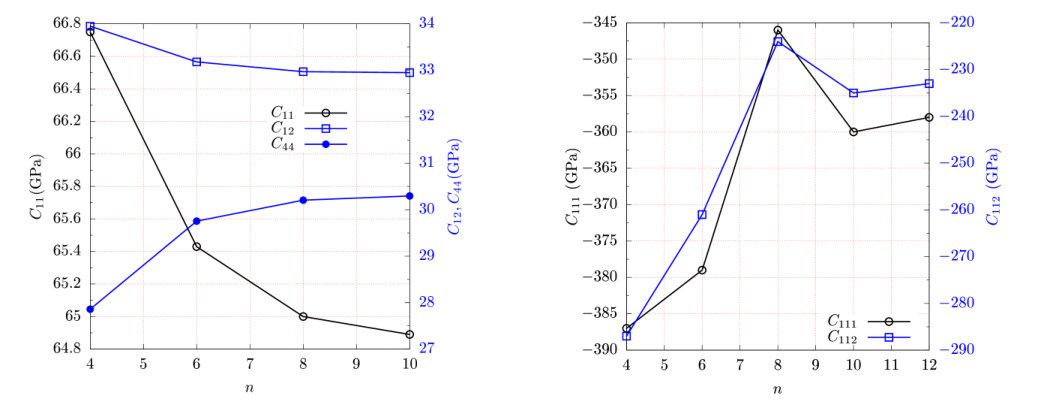 Figure 1
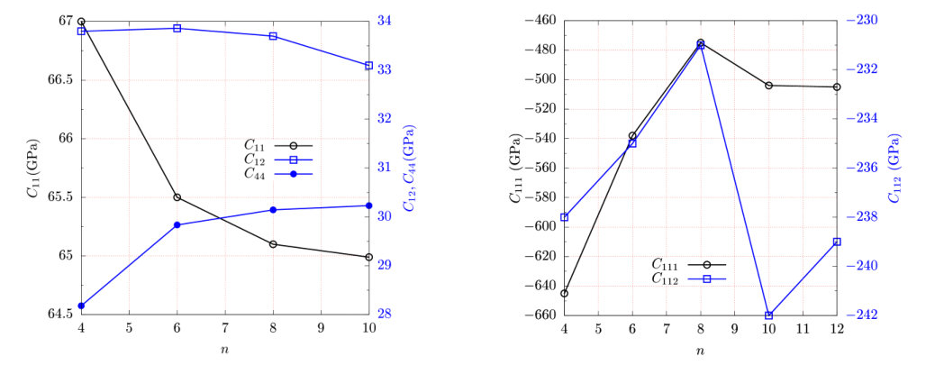 Figure 2
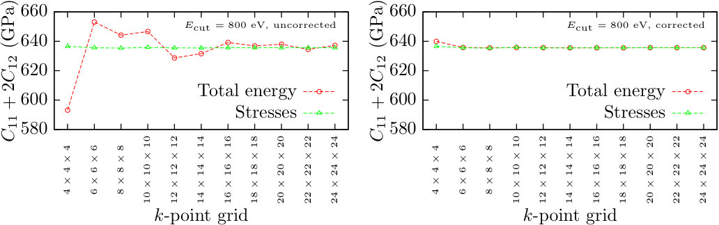 Figure 3
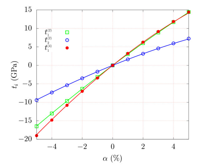 Figure 4
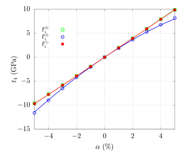 Figure 5
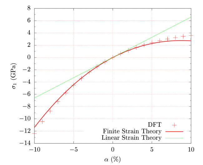 Figure 6
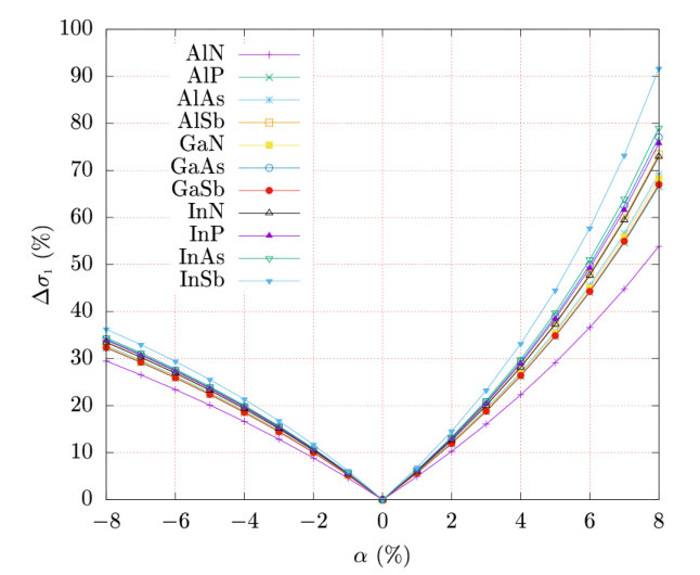 Figure 7
| 400 | 65.20.1 | 65 1 | 379 11 | 1108 15 |
|---|---|---|---|---|
| 600 | 64.890.03 | 65.0 0.2 | 360 4 | 504 34 |
| 1000 | 64.8 0.1 | 64.9 0.1 | 359 6 | 445 21 |
| (Å) | (kB) | (GPa) | (GPa) | (GPa) |
|---|---|---|---|---|
| 4.3643 | 0.5927 | 3103 | -1471169 | -11223 |
| 4.3646 | 0.1521 | 309.560.40 | -121243 | -11233 |
| 4.3647 | 0.0051 | 309.490.03 | -11253 | -11223 |
| 4.3648 | 0.1369 | 309.410.37 | -103740 | -11183 |
| 4.3651 | 0.5752 | 3092 | -778164 | -11174 |
| (1000 eV) | ||||
|---|---|---|---|---|
| 2% | 309.49 0.03 | 1125 3 | 2959 381 | 1223 22 |
| 4% | 310.0 0.1 | 1125 6 | 1627 80 | 1153 6 |
| 6% | 310.8 0.2 | 1126 8 | 1359 31 | 1137 5 |
| 8% | 311.9 0.3 | 1128 9 | 1261 17 | 1132 5 |
| (Å) | (GPa) | (GPa) | (GPa) | |||
| Prev theory | 4.342Wright and Nelson (1995) | 304Wright (1997), 282Łopuszyński and Majewski (2007) | 160Wright (1997), 149Łopuszyński and Majewski (2007) | 193Wright (1997), 179Łopuszyński and Majewski (2007) | 0.55Wright (1997) | |
| AlN | Experimental | 4.373As (2010), 4.38Petrov et al. (1992) | - | - | - | - |
| Present | 4.3647 | 309.47 | 166.06 | 196.90 | 0.5385 | |
| Prev theory | 5.417Wang and Ye (2002), 5.4735Singh (1993) | 132.5Wang and Ye | 66.7Wang and Ye | 62.7Wang and Ye | 0.604Wang and Ye | |
| AlP | Experimental | 5.46Bessolov et al. (1982), 5.4635Madelung (2003) | - | - | - | - |
| Present | 5.4713 | 138.25 | 67.73 | 66.52 | 0.5759 | |
| Prev theory | 5.614Wang and Ye (2002) | 113.1Wang and Ye | 55.5Wang and Ye | 54.7Wang and Ye | 0.592Wang and Ye | |
| AlAs | Experimental | 5.66139Madelung (2003) | 119.9Madelung (2003) | 57.5Madelung (2003) | 56.6Madelung (2003) | - |
| Present | 5.6865 | 116.64 | 55.62 | 56.96 | 0.5746 | |
| Prev theory | 6.090Wang and Ye (2002) | 85.5Wang and Ye | 41.4Wang and Ye | 39.9Wang and Ye | 0.601Wang and Ye | |
| AlSb | Experimental | 6.1355Madelung (2003) | 87.7Madelung (2003) | 43.4Madelung (2003) | 40.76Madelung (2003) | - |
| Present | 6.1877 | 86.39 | 40.65 | 40.71 | 0.5893 | |
| Prev theory | 4.460Wright and Nelson (1994) | 293Wright (1997), 252Łopuszyński and Majewski (2007) | 159Wright (1997), 129Łopuszyński and Majewski (2007) | 155Wright (1997), 147Łopuszyński and Majewski (2007) | 0.61Wright (1997) | |
| GaN | Experimental | 4.50597Frentrup et al. (2017), 4.510Novikov et al. (2010) | - | - | - | - |
| Present | 4.4925 | 288.35 | 152.98 | 166.68 | 0.5678 | |
| Prev theory | 5.463Råsander and Moram (2015), 5.322Wang and Ye (2002) | 142Råsander and Moram (2015), 150.7Wang and Ye | 61Råsander and Moram (2015), 62.8Wang and Ye | 72Råsander and Moram (2015), 76.3Wang and Ye | 0.516Wang and Ye | |
| GaP | Experimental | 5.439Madelung et al. (1998) | 140Madelung et al. (1998) | 62Madelung et al. (1998) | 70Madelung et al. (1998) | - |
| Present | 5.4600 | 142.16 | 60.47 | 72.58 | 0.5333 | |
| Prev theory | 5.619Sörgel and Scherz (1998), 5.75Łopuszyński and Majewski (2007) | 125.6Sörgel and Scherz (1998), 99Łopuszyński and Majewski (2007) | 55.06Sörgel and Scherz (1998), 41Łopuszyński and Majewski (2007) | 60.56Sörgel and Scherz (1998), 51Łopuszyński and Majewski (2007) | 0.514Sörgel and Scherz (1998) | |
| GaAs | Experimental | 5.65325Blakemore (1982) | 113Blakemore (1982), 120Madelung et al. (1998) | 57Blakemore (1982), 53Madelung et al. (1998) | 60Blakemore (1982), 60Madelung et al. (1998) | 0.55Cousins et al. (1989a) |
| Present | 5.6859 | 116.81 | 49.64 | 59.76 | 0.5288 | |
| Prev theory | 5.981Wang and Ye (2002) | 92.7Wang and Ye | 38.7Wang and Ye | 46.2Wang and Ye | 0.530Wang and Ye | |
| GaSb | Experimental | 6.0959Madelung (2003) | 88.34Madelung (2003) | 40.23Madelung (2003) | 43.22Madelung (2003) | - |
| Present | 6.1524 | 86.37 | 36.55 | 43.44 | 0.5517 | |
| Prev theory | 4.932Wright and Nelson (1995) | 187Wright (1997), 159Łopuszyński and Majewski (2007) | 125Wright (1997), 102Łopuszyński and Majewski (2007) | 86Wright (1997), 78Łopuszyński and Majewski (2007) | 0.80Wright (1997) | |
| InN | Experimental | 4.98Strite et al. (1993), 5.01Schörmann et al. (2006) | - | - | - | - |
| Present | 4.9908 | 185.20 | 121.72 | 91.49 | 0.7474 | |
| Prev theory | 5.899Råsander and Moram (2015), 5.729Wang and Ye (2002) | 101Råsander and Moram (2015), 109.5Wang and Ye | 54Råsander and Moram (2015), 55.7Wang and Ye | 48Råsander and Moram (2015), 52.6Wang and Ye | 0.615Wang and Ye | |
| InP | Experimental | 5.8687Madelung (2003) | 101.1Madelung (2003) | 56.1Madelung (2003) | 45.6Madelung (2003) | - |
| Present | 5.9035 | 100.42 | 53.72 | 47.39 | 0.6520 | |
| Prev theory | 6.103Råsander and Moram (2015), 5.921Wang and Ye (2002) | 86Råsander and Moram (2015), 92.2Wang and Ye , 72Łepkowski (2008) | 45Råsander and Moram (2015), 46.5Wang and Ye , 43Łepkowski (2008) | 40Råsander and Moram (2015), 44.4Wang and Ye , 33Łepkowski (2008) | 0.598Wang and Ye | |
| InAs | Experimental | 6.0583Madelung (2003) | 83.29Madelung (2003) | 45.26Madelung (2003) | 39.59Madelung (2003) | - |
| Present | 6.1160 | 84.28 | 44.72 | 39.66 | 0.6378 | |
| Prev theory | 6.542Råsander and Moram (2015), 6.346Wang and Ye (2002) | 67Råsander and Moram (2015), 72.0Wang and Ye | 34Råsander and Moram (2015), 35.4Wang and Ye | 30Råsander and Moram (2015), 34.1Wang and Ye | 0.603Wang and Ye | |
| InSb | Experimental | 6.4794Madelung (2003) | 69.18Madelung (2003) | 37.88Madelung (2003) | 31.32Madelung (2003) | 0.68Cousins et al. (1991) |
| Present | 6.5625 | 64.97 | 33.00 | 30.42 | 0.6366 |
| (GPa) | (GPa) | (GPa) | (GPa) | (GPa) | (GPa) | |
|---|---|---|---|---|---|---|
| AlN | -11253 | -10368 | -4412 | 513 | -7893 | -11.60.7 |
| AlP | -5954 | -4284 | -1036 | 14.90.9 | -2431 | -331 |
| AlAs | -5264 | -3643 | -864 | 7.10.7 | -2201 | -271 |
| AlSb | -4163 | -2682 | -773 | 6.40.5 | -156.90.6 | -21.40.7 |
| GaN | -12778 | -9764 | -2529 | -461 | -6472 | -491 |
| GaP | -7538 | -4417 | -737 | -101 | -2951 | -471 |
| GaAs | -6125 | -3514 | -865 | -15.20.9 | -2641 | -331 |
| GaSb | -4716 | -2605 | -634 | 51 | -1921 | -19.30.3 |
| InN | -7868 | -7018 | -32712 | 282 | -2901 | 221 |
| InP | -4912.5 | -3362 | -1313.5 | -5.170.59 | -168.60.6 | -13.60.6 |
| InAs | -40616 | -26215 | -13213 | -8.80.6 | -1561 | -7.90.7 |
| InSb | -3604 | -2353 | -943 | -142 | -1221 | -6.80.8 |
| (GPa) | (GPa) | (GPa) | (GPa) | (GPa) | (GPa) | |
|---|---|---|---|---|---|---|
| AlN | 1070a | 965a | 61a | 57a | 757a | 9a |
| GaN | 1213a | 867a | 253a | 46a | 606a | 49a |
| GaP | -67652b,c | -49925b,c | -8256b,c | 7547b,c | -33223b,c | 19966b,c |
| GaAs | 561a,-6189b,d,e | 318a,-3894b,d,e | 70a,-4811b,d,e | 16a,5025b,d,e | 242a,-2683b,d,e | 22a,-3710b,d,e |
| GaSb | -4756f | -3082f | -4429f | 51f | -21613f | -2515f |
| InN | 756a | 636a | 310a | 13a | 271a | 15a |
| InAs | 404g | 268g | 121a | 5g | 138g | 6g |
| InSb | -33830b,h | -24217b,h | -7914b,h | 137b,h | -1317b,h | 03b,h |
| (Å) | (Å) | (Å) | (Å) | |
|---|---|---|---|---|
| AlN | -0.58880.0002 | 4.3390.008 | 4.4780.009 | 2.330.03 |
| AlP | -0.79360.0003 | 4.010.01 | 5.320.01 | 1.810.06 |
| AlAs | -0.81870.0003 | 3.9590.009 | 5.3850.007 | 1.950.06 |
| AlSb | -0.91290.0003 | 3.950.01 | 5.530.01 | 1.720.06 |
| GaN | -0.63940.0002 | 4.040.02 | 6.110.02 | 1.970.02 |
| GaP | -0.72950.0002 | 3.4170.008 | 5.650.01 | 1.980.04 |
| GaAs | -0.75330.0005 | 3.5840.009 | 5.550.01 | 2.380.08 |
| InN | -0.93570.0002 | 5.120.05 | 6.610.04 | 1.230.03 |
| InP | -0.96450.0004 | 3.860.03 | 6.720.03 | 1.440.07 |
| InAs | -0.97770.0004 | 3.910.05 | 6.580.07 | 1.700.06 |
| InSb | -1.04270.0009 | 3.190.25 | 6.610.07 | 1.80.1 |
| GaSb | -0.84990.0002 | 3.480.02 | 5.380.01 | 2.200.03 |
Peer Reviews
No public reviews on file for this paper yet. If you reviewed it on a platform where reviews are public (OpenReview, ICLR, NeurIPS, ICML), you can paste yours below so the community can read it here.
Videos
No videos yet. Explain this paper in a talk, walkthrough, or lecture? Add one.
Hybrid functional study of non-linear elasticity and internal strain in zincblende III-V materials
Daniel S. P. Tanner
Tyndall National Institute, Lee Maltings, Dyke Parade, Cork T12 R5CP, Ireland
Miguel A. Caro
Department of Electrical Engineering and Automation, Aalto University, Espoo 02150, Finland
Department of Applied Physics, Aalto University, Espoo 02150, Finland
Stefan Schulz
Tyndall National Institute, Lee Maltings, Dyke Parade, Cork T12 R5CP, Ireland
Eoin P. O’Reilly
Tyndall National Institute, Lee Maltings, Dyke Parade, Cork T12 R5CP, Ireland
Department of Physics, University College Cork, Cork T12 YN60, Ireland
Abstract
We investigate the elastic properties of selected zincblende III-V semiconductors. Using hybrid functional density functional theory we calculate the second and third order elastic constants, and first and second-order internal strain tensor components for Ga, In and Al containing III-V compounds. For many of these parameters, there are no available experimental measurements, and this work is the first to predict their values. The stricter convergence criteria for the calculation of higher order elastic constants are demonstrated, and arguments are made based on this for extracting these constants via the calculated stresses, rather than the energies, in the context of plane-wave-based calculations. The calculated elastic properties are used to determine the strain regime at which higher order elasticity becomes important by comparing the stresses predicted by a lower and a higher order elasticity theory. Finally, the results are compared with available experimental literature data and previous theory.
pacs:
78.67.De, 73.22.Dj, 73.21.Fg, 77.65.Ly, 73.20.Fz, 71.35.-y
I Introduction
Elastic constants are fundamental material parameters, a knowledge of which is essential for the design and understanding of semiconductor materials and devices. For example, the electronic and optical properties of semiconductor heterostructures are strongly influenced by the strain state of their active regions.O’Reilly (1989) This strain state depends on the lattice mismatch between the constituent compounds, and on the relative magnitude of their elastic constants.Nye (1985) Elastic constants are also necessary for: the determination of the material composition of heterostructures by X-ray diffraction;Moram and Vickers (2009) assessing the critical thickness and strain relaxation in devices;Holec et al. (2007) modeling the behaviour of dislocations;Kittel (2004) the characterisation of piezoelectric resonators;Brand et al. (2015) and the parameterisation of interatomic potentialsKeating (1966a) used for the calculation of strain fields in supercells containing millions of atoms.
For crystals which lack inversion symmetry, standard macroscopic elasticity theory does not fully describe the position of their atoms under strain, and internal strainBorn and Huang (1954); Kleinman (1962); Cousins (1978a) occurs. Internal strain is a displacement between sublattices in a crystal. It is described, for a particular material, by the components of the internal strain tensor. Knowledge of these material parameters is essential for any semi-emprical atomistic modelling which requires the equilibrium atomic positions of strained structures, and has, for instance, particular importance for the piezoelectricity of a crystal.Birman (1958); Martin (1972)
For many device and material applications, infinitesimal strain theory,Landau and Lifshitz (1986) in which there appear only second-order elastic constants (SOEC) and first-order internal strains, is sufficient to describe the elastic properties. This means that the crystal energy can be accurately expressed to second-order in the strain, with the SOECs as coefficients, and that the internal strain can be described accurately to first-order in the strain, with the first-order internal strain tensor components (ISTCs) as coefficients. However, as the strain in the system increases, its energy (internal strain) can no longer be accurately described using only a second (first) order expansion in the strain, and higher order terms need to be accounted for. The lowest order of such corrections are third-order elastic constants (TOEC) for the macroscopic strain energy, and second-order ISTCs for the internal strain. The strain magnitudes at which these corrections to the energy and internal relaxation become important will depend on the relative magnitudes of the higher and lower order coefficients of the strains.
Recent studies have shown that third-order contributions to the elastic energy are necessary to correctly model the relaxation, strain state, and thus optical propeties, of several technologically important heterostructures such as InGaAs/GaAs,Pryor et al. (1998); Frogley et al. (2000); Ellaway and Faux (2002); Ma et al. (2004); Łepkowski (2008) InGaN/GaN, and GaN/AlGaN.Łopuszyński and Majewski (2007); Łepkowski and Majewski (2004); Łepkowski et al. (2005); Łepkowski (2008); Shan et al. (1998) Similar effects can be expected in other highly lattice-mismatched nanostructured systems, such as the InSb/GaSb quantum dot (QD) system.Deguffroy et al. (2007) Furthermore, second-order ISTCs have been shown to play an important role in the piezoelectric response in many materials.Caro et al. (2015); Migliorato et al. (2006) Other phenomena related to lattice anharmonicity, such as: phonon-phonon or electron-phonon interactions;Hiki (1981) thermal expansion;Hiki (1981) stress or temperature dependent elastic response;Hiki (1981) and pressure dependence of optic mode frequencies,Cousins (2001) also require the use of TOECs and second-order ISTCs.
Because of this wide application, there has long been interest in the measurement or theoretical determination of TOECs.Brugger (1964); Keating (1966b); Birch (1947); Wallace (1970) Typically, TOECs are measured using the velocity of sound waves through a crystal under uniaxial or hydrostatic stress,Thurston and Brugger (1964) analysed via the finite strain theory of Murnaghan.Murnaghan (1951, 1937) However, there are often very large uncertainties in such measurements,Johal and Dunstan (2006) and these difficulties are compounded for brittle or metastable semiconductor materials,Cousins (2001); Cousins et al. (1991); Lang and Gupta (2011) which are often of interest for device applications. Similarly, for the internal strain, of the materials addressed in this paper, only GaAs and InSb have available experimental values of their single first order ISTC (Kleinman parameter), due to the high precision of experimental observations requiredCousins (2001); Chandrasekaran et al. for the extraction of ISTCs; there are no experimental evaluations of any second-order ISTCs. Thus, given the experimental difficulty in the measurement of ISTCs in general, and the importance of non-linear elasticity for the accurate description of the electronic and optical properties of technologically relevant semiconductors and their connected heterostructures, there is strong motivation for the theoretical determination of TOECs and first and second-order ISTCs.
Early calculations of TOECs involved the use of pseudopotentialSuzuki et al. (1968) and interatomic force potential methods;Keating (1966b) however, since the work of Nielsen and Martin,Nielsen and Martin (1985) first principles calculations have become an increasingly popular route towards the calculation of TOECs. In recent years, ab-initio methods have been used to determine the TOECs for ultrahard materials such as diamond;Hmiel et al. (2016); Nielsen (1986) materials of which it is difficult to obtain high quality single crystals, like the metastable cubic-phase nitride materials;Łopuszyński and Majewski (2007) and technologically important materials for which experimental TOEC measurements are sparse, such as InAs and GaAs.Sörgel and Scherz (1998); Nielsen and Martin (1985); Łopuszyński and Majewski (2007); Łepkowski (2008)
In this work, we present first-principles calculations of SOECs, TOECs, as well as first and second-order ISTCs, of a range of III-V zincblende (ZB) semiconductor compounds. The calculations are carried out using density functional theory (DFT) within the Heyd-Scuseria-Ernzerhof (HSE) hybrid-functional approach.Heyd et al. (2003) We demonstrate that higher order elastic properties require a higher resolution of calculation parameters for their accurate evaluation, and extend arguments present in the literature for the use of the stress method for the extraction of elastic constants to the case of TOECs. Moreover, we show the importance of third-order effects in the strain regimes relevant to a sample InSb/GaSb heterostructure system, and demonstrate for other materials the errors incurred by the use of a linear theory. Finally, our results are compared, where possible, with previous experimental and theoretical results. Overall, we find very good agreement with previously reported experimental and theoretical literature data.
The paper is organised as follows: in Section II we present the finite strain theory in which the TOEC and second-order ISTCs are defined; in Section III we discuss our computational framework, giving the specifics of the DFT implementation and discuss the different nature of convergence of TOECs compared with SOECs, including a comparison of constants extracted from the stress-strain approach with those extracted via the total energy; in Section IV we present the calculated SOECs, TOECs and first and second-order ISTCs, make comparisons with recent experiment and theory, and apply the extracted TOECs to address the question as to the strain regime in which non-linear elasticity need be used; finally, in Section V, we summarise and conclude.
II Overview of finite strain theory
In this section we review the aspects of finite strain theory necessary for the calculation and discussion of TOECs and second-order ISTCs. In Sec. II.1, we apply finite strain to the discussion of the macroscopic elasticity of crystals, and in Sec. II.2, we outline the theory describing the internal strain resulting from a given applied finite strain.
II.1 Elasticity
In solid state physics, the description of third-order elasticity is conventionally achieved via the Lagrangian strain formalism.Brugger (1964); Nielsen and Martin (1985); Łopuszyński and Majewski (2007); Hmiel et al. (2016) The application of Lagrangian stresses and strains to the theory of elasticity with finite deformations has been developed by Murnaghan,Murnaghan (1937, 1951) and applied to cubic crystals by Birch.Birch (1947)
The deformation gradient tensor, , marks the starting point of all strain formalisms. It describes the deformation of a material, including rotations, when the coordinates of that system are transformed. If the position of a point in a material is given by , and after strain is at the position , then the deformation tensor may be defined as:Nye (1985)
[TABLE]
This relates simply to the linear strain tensor as:
[TABLE]
where is the Kronecker delta, and is the small, or infinitesimal, strain tensor. While this simple relation between the infinitesimal strain and the deformation is very useful and attractive, the conceptual underpinning of the infinitesimal strain (that it measures the relative changes of lengths in the material) becomes increasingly invalid with increasing strain. Thus, in the regime of larger strains, where third-order elasticity becomes relevant, Lagrangian strains are employed. The Lagrangian strain tensor, , is related to the deformation by:Birch (1947)
[TABLE]
where Einstein summation notation is used. In cases where the infinitesimal strain tensor is known, the following useful matrix relation may be used to determine the Lagrangian strain tensor:Birch (1947)
[TABLE]
The TOECs are conventionally defined in terms of the expansion of the free energy density in these Lagrangian strains. For a cubic crystal, this energy density is given by:Brugger (1964); Birch (1947); Łopuszyński and Majewski (2007)
[TABLE]
Here is the mass density of the unstrained material, is the Helmholtz free energy per unit mass, and the various and are the second and third-order isentropic elastic constants, respectively. We have also above employed Voigt Voigt (1928); Nye (1985) notation, which, using the symmetry of the strain tensor, makes the convenient contraction of indices: 111, 222, 333, 324, 135, 126. The derivatives of this energy density, , with respect to the provide equations relating the Lagrangian stresses, , to the Lagrangian strains, , via the elastic constants:
[TABLE]
Thus, the general expressions for the Voigt components of the Lagrangian stress in terms of an arbitrary Lagrangian strain on a cubic crystal are:
[TABLE]
with and , given by cyclic permutations of the indices of and , respectively.
However, when the stresses on a strained supercell are calculated via DFT using the Hellmann-Feynman theoremNielsen and Martin (1983) or from an interatomic potential calculation, it is the stresses on the faces of the deformed cell that are obtained; these are the Cauchy stresses, . Therefore, in order to use eqs.(7) to extract elastic constants from DFT data, the Lagrangian stress must be related to the Cauchy stress:Murnaghan (1951)
[TABLE]
Hence, by either measuring the energy or stress of a cubic crystal as a function of applied Lagrangian strain, eqs. (5) ,(7) and (8) may be used to obtain values for the elastic constants.
Having established the finite strain formalism required for the discussion of TOECs, in the next section we describe the application of this formalism to the description of non-linear inner elasticity in cubic crystals.
II.2 Internal strain
Non-linear internal strain involves a second, rather than first-order description of the internal strain in terms of the Lagrangian strain. To achieve this description of sublattice displacement to second-order in the regime of large strains for ZB semiconductors, we will use the formalism introduced by Cousins.Cousins (1978a, 2001)
Taking the ZB primitive cell, and letting the atom at the origin remain fixed, the position of the second atom, after strain, is given by:
[TABLE]
where is its equilibrium position, and represents the internal strain vector. Although this transformation completely specifies the deformed positions geometrically, the are not suitable parameters in which to expand the scalar energy. This is because they lack rotational invariance. Given that the internal strain represents the atomic configuration which minimises the energy of the ZB crystal under shear strain, a rotationally invariant description of the internal strain is needed. This is obtained through use of what Cousins Cousins (1978a) calls the inner displacement. This is given by:
[TABLE]
Because this inner displacement occurs in response to internal forces arising from the application of finite strain, each inner displacement can be expressed as a Taylor series in the components of the strain:
[TABLE]
Here, Voigt notation has been employed for the elements of the finite strain tensor, and the Einstein summation convention is again utilised. The subscripts relating to the strain are denoted by capitals, whilst those relating to the Cartesian coordinate of the inner displacement are denoted by the lower-case . The and are the first and second-order internal strain tensors, respectively. Cousins Cousins (2001, 1978b) gives the form of these tensors for a ZB crystal. The first-order internal strain tensor may be expressed conveniently in matrix notation:
[TABLE]
We note that for small strains, , the identity matrix, and , where (, , ), and thus , where is the well known Kleinman parameter.Kleinman (1962)
A matrix representation is not possible for , but there are only three independent non-zero components which are:Cousins (1978b)
[TABLE]
Substituting eqs. (12)-(15) into eq. (11) yields an expression for the value of which minimises the strain energy of a ZB crystal for a given applied finite strain:
[TABLE]
If, for a given primitive ZB unit cell, the atomic positions corresponding to the energetic minimum for a particular Lagrangian strain branch are known, eq. (16) can be used in fitting procedures to obtain the first and second-order ISTCs.
In the next section, the manner in which the presented finite strain theory is applied to deformed unit cells is described. In addition, the details of the DFT caculations performed to obtain the stresses on, and energies of, these deformed unit cells are presented, along with a discussion of the different calculational criteria needed for the accurate calculation of elastic constants and internal strain tensor components.
III Computational Method
In this section we discuss the computational method used to calculate the SOECs, TOECs and first and second-order ISTCs.
First, in Sec. III.1, the deformations applied to each ZB unit cell are presented. This is accompanied by a description of the strains and stresses associated with these deformations via the finite strain theory introduced in the previous section. In Sec. III.2, the details of the DFT calculations are given. This is followed in Sec. III.3 by an analysis of the convergence of the calculations with respect to k-point grid density, plane-wave cutoff energy, lattice constant, and applied strain range. In particular, it is demonstrated and explained that a higher resolution of calculation in terms of k-point grid density, cutoff energy, and lattice constant, is needed to achieve convergence of TOECs when compared with that needed for the calculation of SOECs. Whether to calculate the elastic constants via the calculated stresses or energies is discussed. Our results show that, using the energy method, the convergence of TOECs is much slower with respect to cutoff energy, k-points and applied strain range when compared to that exhibited by the stress strain method. Consequently, the energy method is significantly more computationally expensive. A similar behaviour has been reported in the literature for SOECs,Caro et al. (2013) where it was identified that the slower convergence of the energy method occurs due to changes in the k-point basis set used, as the cut-off energy is kept fixed in the calculations, while the unit cell size/shape is being varied. By contrast,the stresses, when calculated according to the Hellmann-Feynmann theorem, are computed implicitly for a fixed basis set (since they are computed at fixed lattice vectors). We then find, given the already high computational demands, that the effect of the changing basis set in the energy calculations is strongly enhanced when calculating TOECs, as further discussed in Section III.3.1.
III.1 Applied deformations
For the extraction of all SOECs, TOECs, and first and second-order ISTCs, data from the following applied strain branches Caro et al. (2015) were used:
[TABLE]
The corresponding deformations of the unit cell were chosen such that, according to the symmetries of eqs. (12)-(16), at least one independent determination of each of the second-order ISTCs would be obtained from the resultant inner displacements. Deformations chosen in this way also enabled several pathways to the determination of each of the SOECs and TOECs from the stresses on the unit cells.
For the calculation of all elastic constants and ISTCs, and are varied in the following manner: In the strain branch , is varied in steps of 0.01 from 0.04 to 0.04, resulting in a total of 9 strain points. For each of the remaining branches, () is varied from 0.02 (0.04) to 0.02 (0.04) in steps of 0.01 (0.02), comprising a total of 25 points. Each value of and is associated with six stress components, a total energy value, and the position vectors of the atoms in the ZB primitive cell. To ascertain the form of the relation between the deformation parameters and , and the stress, energy, and relaxed atomic positions, the Lagrangian strains corresponding to each deformation branch must be determined. Using the tensor relation, eq. (4), the Lagrangian strains, , obtained from the strain branches, , are given by:
[TABLE]
where the notation and , has been used for compactness.
With these five strain branches there are: five energy equations from eq. (5), from which all SOEC and TOECs may be obtained; fourteen unique stress component equations, from which all SOEC and TOEC may be obtained in multiple ways using eqs. (7); and five equations for inner displacements, from eq. (16). We do not present these twenty four long equations here in the interest of brevity. However, to illustrate the methodology, we will present in the results section a sample subset of these equations, truncated to second order in the deformation parameters. A more detailed description of the full set of stress and inner displacement fitting equations is given in Ref. [tanner, 2017].
The first three of the Lagrangian strain branches of eq.( 18) allow, via the relaxed atomic positions, determination of (the Kleinman parameter within the finite strain formalism, ), and all three of the second-order ISTCs. Furthermore, because and are varied independently, these first three branches also furnish, via the different components of the stress tensor, multiple independent determinations of each of the SOECs, and all but one of the TOECs. The remaining TOEC, , can then be determined from the stress in the direction associated with . The stresses and relaxed atomic positions of the more complicated strain branch, , are not used to obtain any new values for the elastic constants, but to check the overall accuracy and consistency of the full set of elastic constants or ISTCs by substituting in particular values derived from the other branches, and performing fits for the remaining constants. Since the fitting will be dependent on the accuracy of the substituted constants, the agreement of the result with previous fittings indicates accurate determination of all those substituted constants, as well as those newly obtained.
III.2 DFT framework for the calculation of energy, stress, and relaxed atomic positions
To obtain the energies, stresses, and relaxed atomic positions associated with each of the above strain branches, DFT calculations were performed on the (deformed) ZB unit cells using the Heyd-Scuseria-Ernzerhof (HSE) hybrid-functional approach.Heyd et al. (2003) The calculations were carried out using the software package .Kresse and Furthmüller (1996) A screening parameter, , of 0.2 Å*-1*, and an exact exchange mixing parameter, , of 0.25, were utilised; these correspond to ’s HSE06 version of the HSE functional. More details are given in Ref.[Caro et al., 2015].
For the calculation of material parameters, DFT within the HSE scheme offers improved accuracy over standard Kohn-Sham approaches to the exchange energy.Henderson et al. (2011) For instance, it circumvents the well known band gap problem of LDA and generalised gradient approximation (GGA) implementations. Moreover, HSE-DFT has been shown to give improved predictions of elastic and lattice properties of solids over LDA and GGA implementations.Paier et al. (2006); Råsander and Moram (2015) Fitting to the DFT data using eqs. (5), (7) and (16), yields values for the SOECs and TOECs as well as first and second-order ISTCs as described above.
For the determination of elastic constants, we choose to fit to the stress-strain equations (eq. (7)) rather than the energy-strain equations (eq. (5)) for reasons of greater accuracy and efficiency,Caro et al. (2013); Nielsen and Martin (1983, 1985); Hmiel et al. (2016) which we will demonstrate below. In general, the stress method is suited to efficient calculation of the elastic constant tensor because a single DFT calculation yields the full stress tensor, with its six unique components, and six equations to fit to. However, a single DFT calculation produces only one scalar energy, with one equation available to fit to. Thus the elastic constants can be obtained via the stress method efficiently from one calculation, whereas from the energy method, several separate calculations are needed for the same number of constants. Furthermore, in terms of accuracy, the equations relating these elastic constants to the strains will be a lower order polynomial in the strain, and therefore easier to fit when dealing with very small strains. Finally, as will be corroborated in the next section: in a plane wave-based DFT implementation using a fixed cutoff energy in its plane-wave expansion at different k-points and different lattice vectors, the number of k-points and cutoff energy needed in a given calculation to obtain converged values of the elastic constants is lower for those calulated via the stress method than for those calculated via the total energy method.Caro et al. (2013) Consequently, elastic constants can be determined to a desired accuracy at less computational expense using the stress method. Moreover, these issues of convergence are even more pronounced for TOECs and second-order ISTCs than SOECs and first-order ISTCs, as will be demonstrated below.
III.3 Convergence of Results
In this section, we analyse the convergence of our results, and show that the aforementioned advantages in convergence which the stress method exhibits over the energy method, demonstrated in the literature in the context of SOECs,Caro et al. (2013); Nielsen and Martin (1983, 1985) are even more dramatic for the TOECs. First, in Sec III.3.1, we show that TOECs require a higher resolution of calculation than SOECs: that elastic constants extracted via the stress method converge faster with respect to k-point mesh density and cutoff energy than those extracted via the energy method; and that the elastic constants presented here, calculated using the stress method, are converged (where those extracted via the energy method, from the same calculation, may not be). These convergence tests are shown using InSb as a model system, which of the studied materials is the slowest to converge with k-point density and cutoff energy. Thus, the presented results for InSb validate also the convergence of the other III-V materials studied here. Second, in Sec. III.3.2 the dependence of the extracted elastic constants on the equilibrium pressures and applied strain ranges is investigated. The increased sensitivity of TOECs to these calculation parameters when compared with SOECs is highlighted, and this increased sensitivity is shown to be worsened when elastic constants are extracted through use of the energy method. Finally, the suitability of our choice of applied strain range and allowed equilibrium pressure are confirmed.
III.3.1 Convergence with k-points and cutoff energy
Compared to the effects of linear elasticity, third-order elasticity gives rise to smaller changes in stress, energy, and atomic positions. Therefore, it can be expected that convergence of TOECs will require denser k-point grids and higher cutoff energies than is the case for SOECs. We find that this is indeed the case, as illustrated in Fig. 1, where, for InSb, the slower convergence of the stress-extracted TOECs with respect to k-point density may be immediately inferred from the different scales. Here the cutoff energy is fixed at 600 eV. On closer inspection of Fig. 1, one finds that the percentage changes in and on going from a to an k-point grid are both 1%, whilst for and the values change by 10% and 17%, respectively. Therefore, while an k-point grid may be sufficient to obtain converged SOECs, the calculation of TOECs requires a higher k-point density. Examining the percentage change in the calculated constants when going from an to a k-point mesh, convergence of both SOECs and TOECs is apparent. For the SOECs a negligible difference of 0.5% exists, whilst for the TOECs, and , the values differ by only 4% and 5%, respectively. To further corroborate convergence of the TOECs, we note the negligible change on increasing the k-point density from to ; the differences being 1% for both TOECs. With these small changes between subsequent grid sizes, we conclude that a grid of is sufficient to converge the stress extracted elastic constants, at a cutoff energy of 600 eV.
While Fig. 1 establishes convergence of the elastic constants extracted through the stress method, Fig. 2 justifies the choice of extracting the elastic constants using the stress rather than energy by showing the poorer convergence of the energy method. Figure 2 shows that, using the energy method, the TOECs also converge much slower when compared with the SOECs. Also similarly to the convergence of the stress-extracted constants, the energy-extracted TOECs are also clearly converged with respect to k point density by a k-point grid density. However, in this case, the TOECs exhibit much larger fluctuations at lower grid densities. For example, at a grid of , the energy extracted is 28% lower than the converged value, whilst the stress-extracted is only 8% lower than its converged value. In addition to the fact that the energy values are converging slowly, we note, more importantly, that they are also unconverged at this cutoff energy, with final and values of -504 and -242 GPa, respectively, compared to the converged stress-extracted values of -360 and -235 GPa.
Therefore, in a second step, we analyse the impact of the cutoff energy on the elastic constants. Table 1 shows the effect of increasing the cutoff energy, with a fixed k-point grid of , on the calculated and values. The superscripts, , and , refer to constants extracted via the stress and energy methods, respectively. The numbers following the “” are the fitting errors. The table shows that for both the energy and stress method, a cutoff of 400 eV is more than sufficient to obtain converged SOECs. However, for the TOEC , only the stress extracted is converged. As with Figs. 1 and 2, the table shows that: TOECs generally require higher cutoff energies than SOECs; energy extracted TOECs require higher cutoff energies for a given accuracy than stress extracted TOECs; that a cutoff energy of 600 eV is sufficent to obtain converged TOECs (for InSb) using the stress method; and that even for a cutoff energy of 1000 eV, the energy method still does not yield a converged value for , as can be seen by comparison with .
The slower convergence of the energy extracted parameters with respect to those extracted via the stresses is due to the larger impact of the changing plane-wave basis set on the strain energy than on the stress.Caro et al. (2013) The total energy results can in principle be corrected by using a (in general anisotropic) strain-dependent cutoff energy. For small strains, change in lattice vectors corresponds to change in cutoff energy. This is because, for a cutoff energy , only those plane waves that obey the condition , where is a reciprocal lattice translation, are included in the basis, with:
[TABLE]
Modifying the cut-off energy to maintain a fixed basis set leads to a remarkably improved agreement between total energy and stress methods, as shown in Fig. 3, where, to illustrate this point we have performed LDA calculations of the bulk modulus of AlN using energy and stress, with and without the cutoff energy correction.
Unfortunately, this cut-off energy correction can only be easily implemented for hydrostatic strain (i.e. only allows to calculate bulk modulus) because this is the only case where the basis set changes isotropically, consistent with eq. 3. Because it avoids these issues, the stress method should therefore be used for reliable, consistent, and computationally inexpensive calculation of elastic constants.
Finally, we note that InSb, being the heaviest and softest material, will require the highest resolution of calculation in terms of cutoff energy and k-point mesh. Thus, the convergence indicated in Fig. 1 and Table 1 also serves to confirm that the chosen cutoff energy and k-point density are appropriate for the other materials.
III.3.2 Convergence with applied strain range and equilibrium pressure
In addition to their sensitivity to k-point grid density and cutoff energy, TOECs also exhibit a more pronounced dependence on the residual pressure at the assumed equilibrium lattice constant, and the range of strain applied to the system in order to calculate them. Because the demonstration of this point requires a large number of calculations, in this section we analyse the TOECs and SOECs of AlN. For this compound of lighter atoms, the stress and total energy calculations are computationally less expensive than for InSb. Unless stated otherwise, all convergence tests are performed at a cutoff energy of 600 eV and on a k-point mesh.
The issue of lattice constant relaxation is examined in Table 2, where the elastic constants and , extracted using the stress method, are shown for different equilibrium lattice constants and pressures. The and values displayed are the result of applying the strain branch with varied from to in steps of . The pressure denoted by in the table is the calculated residual pressure on the ZB primitive cell with the lattice constant given in the first column. The values preceded by the “” are least squares fitting errors.
Table 2 shows that, when optimising the lattice constant by minimising the absolute value of the pressure on the unit cell, the magnitude of the pressure below which we may accurately extract elastic constants from the stress, using standard fitting methods, is lower for TOECs than for SOECs. In columns three and four of Table 2 are presented the results of fitting the equation directly to the DFT data, which include this ’equilibrium’ pressure, , as the pressure corresponding to a strain of 0%. Here the variation of AlN’s value with residual “equilibrium” pressure may be contrasted with the constancy of the corresponding value. As the residual pressure increases, so does the value of deviate from the value obtained at lowest pressure, along with increasing fitting errors. For a lattice constant change of -0.0004 Å from the lowest pressure lattice constant, a 30% error is incurred in . This may be attributed to related factors such as: the small magnitudes of the contribution of the TOEC to the total stress (at , =2.25 kB), of which the initial pressure is a significant fraction; and the tendency of higher order polynomials to be more sensitive to noise in fitting.
The errors so-incurred can be reduced by two means. The first is to modify the fitting equation to account for the equilibrium pressure; i.e. by fitting using the equation: . The improvements induced by this adjustment are evident in the stability with intial pressure of in column five of Table 2. The second way to reduce these errors is to ensure the lattice has been relaxed to a sufficiently low pressure; while the origin adjustement shown before more than solves the problem for AlN over the given pressure range, for softer materials, this sensitivity to initial pressure will be even more pronounced, with a given pressure corresponding to a higher strain, and this adjustement is less effective. We thus impose more stringent criteria on the maximum pressures below which we consider a crystal to be relaxed, aiming for pressures below 0.1 kB, a fifth of the cutoff value of 0.5 kB typically used for SOECs.Golesorkhtabar et al. (2013)
Another important calculation parameter to which the TOECs are sensitive is the range of strain applied to the unit cell.Hmiel et al. (2016); Golesorkhtabar et al. (2013) Applying strains over a larger range will produce larger changes in stress and energy from which the contribution of the third-order terms will be more easily discerned; however, as the strain range is increased, even higher order terms may begin to have an effect. Furthermore, having a large strain range with a constant strain point density will require a larger number of calculations. Thus, the strain range applied will need to be large enough that the effect of the TOECs can be observed, but not so large that further higher order terms come into play, or the calculation is prohibitively expensive; i.e., the optimal strain range is the minimum strain range at which the effects of TOECs are appreciable.
Table 3 shows the influence of the range of applied strain on the calculated elastic constants of AlN. The superscript in this table refers to a stress extracted constant, and denotes an energy extracted constant. denotes the maximum value of in the applied strain of , with the data set comprising strains in increments of 1% between . The stability of the stress extracted and in Table 3 reveals that the range of % is large enough to yield measurable non-linearities in the stress, but not so large that higher order terms interfere with the fitting. The increasing influence of these unwanted higher order terms can be observed in the increasing errors of . The rightmost two columns of the table show again the shortcomings of the energy method when compared with the stress method for the extraction of TOECs; the energy extracted constants requiring larger strain ranges to lower the fitting error. The rightmost column shows the interrelation between the cutoff energy and the strain range. Small errors in the calculated free energy can have significant impact on the determined TOECs at small strain; increasing the cutoff energy reduces the scale of these errors, while increasing the strain range reduces their relative input in the total calculated change in energy. Overall, we see that the convergence of the TOEC values is clearly slower using the energy method.
Having justified our choice of the stress method over the energy method for the extraction of SOECs and TOECs, and shown that our stress extracted constants are indeed converged, we present in the next section the full set of SOECs and TOECs for all considered materials, and discuss the results.
IV Results
In this section the calculated SOECs, TOECs and first and second-order ISTCs are presented and discussed. First, in Section IV.1, the calculated elastic constants are presented, along with plots validating the fittings used to obtain them. The extracted values are compared with previous experimental and theoretical literature results, and an analysis of the strains at which third-order effects become important is made. In Section IV.2, the calculated first and second ISTCs are reported.
IV.1 Elastic constants
Given below in eqs. (20) and (21), are six sample stress fitting equations, truncated to second-order in the strain, each furnishing an independent determination of a subset of the nine independent elastic constants of a ZB crystal. Eqs. (20) show three axial stress equations which may be used to determine simultaneously the SOECs: and ; and the TOECs: , and .
[TABLE]
and eqs. (21) show three shear stresses which yield simultaneously values of the SOEC , and TOECs , and :
[TABLE]
Here the subscripts on the refer to the stress tensor component in Voigt notation, and the superscripts, , refer back to the strain branches, , in eq. (18). The zeros in brackets in eq. (21) indicates that is set to 0, and only is varied.
The solid lines in Figs.4 and 5 show the stresses on AlN unit cells as a function of strain, calculated using the expressions in eqs. (20) and (21). The figures also display the stresses calculated by DFT for each strain as symbols. Note that the fitting of the coefficients in eqns. (20) and (21) is not done on the data sets shown in the figure. These coefficients were obtained by two-dimensional fittings to unsimplified untruncated stress equations using only data points in the range: and . The lines shown in the figure show then predictions for higher strain values. As the figures confirm, not only is the fit very good at , but the line also matches the DFT data points very well at higher strains. The influence of non-linear effects may be inferred from the slight curvature and asymmetry of the lines.
By performing fittings to several stress relations, the full set of SOECs and TOECs for all considered materials were obtained. For and , there are two independent determinations, from and , and the values given in Tables 4 and 5 are the averages of these two. The constants and have three independent determinations, , and the values given in the table are the averages of these. is obtained from the single fitting to . For , we extracted six separate values from the different stresses on the unit cells; the value given is the average of all these very closely agreeing values. is given as an average over the values obtained from the three stresses , , and . Finally, for all materials, and were obtained from .
Table 4 presents a comprehensive comparison with experiment and previous theory of lattice constants, SOECs, and Kleinman parameters for all considered materials. The table reveals an abundance of both experimental and theoretical values of lattice and elastic constants for all materials except for the metastable III-N compounds and highly toxic AlP, for which experimental elastic constants are not available. For the Kleinman parameter, experimental values are rare, with measurements made only on GaAsCousins et al. (1989a) and InSbCousins et al. (1991). The theoretical values presented are from DFT studies utilising different approximations to the exchange correlation energy functional. Refs. Wang and Ye, 2002, ; Wright and Nelson, 1994, 1995; Wright, 1997; Sörgel and Scherz, 1998 use the local density approximation (LDA) to the exchange correlation functional. As is evident from the table, in most cases LDA DFT accounts well for the elastic properties of solids; however, LDA is known to often overestimate the binding in solids,Råsander and Moram (2015) resulting in smaller lattice and larger elastic constants. Indeed, we see from Table 4 that whenever there is a significant disagreement between LDA elastic or lattice constants and those experimentally measured or here calculated, the LDA elastic constants tend to be larger. For the Al containing compounds considered here this trend seems not to hold, with the elastic constants being often smaller than experiment, but nevertheless agreeing very closely. Refs Łopuszyński and Majewski, 2007; Łepkowski, 2008 use the generalised gradient approximation (GGA) of Purdew, Burke and Ernzerhof (PBE)Perdew et al. (1996). This functional tends to underestimate binding energiesRåsander and Moram (2015); Łopuszyński and Majewski (2007), and examining in particular InAs and GaAs, we see this trend borne out. From Ref. Råsander and Moram, 2015, we take those structural and elastic properties calculated using HSE; these show good agreement with the HSE-DFT values of the present study, and with experimental values. This good agreement with experiment demonstrates both the validity of the particular HSE-DFT determined elastic constants presented here, and of the use of this method for the calculation of structural and elastic properties in general.
The TOECs, averaged over the independent determinations given in eqs. (7) and (18), are gathered in Table 5. The errors following the constants are the fitting errors.
In Table 6 experimental and theoretical values are provided for those materials for which they are available, with theoretical values italicised. We find good agreement between the experimental measurements and our calculated values, taking into account that these measurements are performed often at room temperature ( K) where materials tend to be softerŁopuszyński and Majewski (2007) than at the K temperature at which DFT calculations are made. With regard to literature theoretical calculations, for GaAs, there were several different works calculating TOECs.Łopuszyński and Majewski (2007); Sörgel and Scherz (1998); Nielsen and Martin (1985); Łepkowski (2008) Here, we present only the most contemporary study, by Łopuszyński and Majewski.Łopuszyński and Majewski (2007) Overall, we find very good agreement between our results and those obtained via experiment or theory in the literature. This serves as a validation for the extracted constants for which previous experimental or theoretical values are not available.
With the TOECs and SOECs thus determined and validated against previous experimental and theoretical values, we may use them to address the question of when third-order effects become important in the materials under consideration. As a test case, we consider an InSb system that is strained in the plane and free to relax in the direction. In Fig. 6, the Cauchy stress, , in the direction, of this system is shown. This stress will be relevant to the pressure tuning of the Poisson ratio, and through this the pressure coefficient of the band-gap. The figure plots the Cauchy stress, determined three different ways, against the strain. The stress obtained from DFT is given by the symbols, that obtained by linear strain theory is given by the thin green line, and that obtained through third-order finite strain theory is given by the solid red line. Figure 6 shows clearly the increasing failure of the linear theory with increasing strain. By 5% strain, the linear theory suffers from errors in of for strain, and for strain. This failing of the linear theory at these strains would introduce inaccuracies in the modelling of, for example, the elasticity of InSb/GaSb quantum wellsQian and Wessels (1993) and QDsDeguffroy et al. (2007) grown by the Stransky-Krastanov method, given that the lattice mismatch between InSb and GaSb is 6.3%.
Extending this analysis to the other materials, in Fig.7, the error in the out of plane stress induced by a biaxial strain as calculated by the linear strain theory when compared with the non-linear theory is plotted as a function of applied strain. From the figure we infer that once the strain in the system is greater than 2%, the linear theory is no longer appropriate, with the errors in the stress being 10% for all materials, except for AlN, which has a 9% error in the calculated stress at 2% strain. These large non-linearities in the out of plane stress will manifest most noticeably in the pressure dependent behaviour of these materials in their respective heterostructures. Indeed, this has been already demonstrated by ŁepkowskiŁepkowski (2008). From our results we may infer that the pressure tuning of strains in InSb/GaSb structures will be even more markedly non-linear than that which has already been observed in InAs/GaAs and InN/GaN systems.
In the next section we turn to higher order effects in the internal strain.
IV.2 Internal strain tensor components
The components of the internal strain tensor are derived from eqs. (16) and (18). These are given for the strain branches, , , and , in eq. (22) below:
[TABLE]
The extracted non-zero components of the internal strain tensor are given in Table 7. For the values from strain branches , and , obtained from fitting to eq.( 22) are averaged. Since there is not the same abundance of equations from the relaxed atomic positions to describe the higher order internal strain tensor components as there are from the stresses for the elastic constants, the values for the different are set simply to those of the single independent determination of lowest error. For the only independent determination is that from ; for , it is . For there are two independent determinations, but we include in the table only the value from the uncomplicated strain branch.
In terms of comparison with previous calculation or measurement, Table 4 reveals very good agreement between our calculated first-order ISTC (the Kleinman parameter) and literature values. To the best of our knowledge, the only other first principles calculation of the components of the second-order internal strain tensor, in diamond or zincblende materials, are those obtained for C in Ref. Nielsen, 1986. Strain derivatives of the Kleinman parameter are available for Si in Ref. 40, and for GaAs in Ref. 25. While these strain derivatives for the case of GaAs could be related to our data in Table 7, we find that the obtained Kleinman parameter of Ref. 25, 0.455, disagrees significantly with our obtained value, 0.5288, with those from experiment, 0.550.02,Cousins et al. (1989b) and with those from more recent theory 0.514,Sörgel and Scherz (1998) 0.517;Raynolds et al. (1995) we do not therefore attempt explicit comparison.
V Conclusion
In summary, second- and third- order elastic and first- and second- order internal strain tensor components were extracted from accurate HSE DFT calculations. The elastic constants and internal strain tensor components were extracted via stress-strain and position-strain relations expressed within the formalism of finite strain, respectively. This is the first determination of many of these constants. In particular, the components of the second-order internal strain tensor extracted here have not before been measured or calculated. Where previously determined, good agreement was obtained with experiment and theory found in the literature. The results of convergence checks presented illustrate that far greater care must be taken in the determination of third-order elastic constants (TOECs) as compared to second-order elastic constants (SOECs), with a high resolution of calculation required. The use of the stress-strain equations for the calculation of elastic constants was justified, and arguments from the literature, formulated in the context of SOECs, were shown to have even more force in the case of third-order elastic constants. The impact of non-linear strain effects was demonstrated in particular for the elasticity of InSb, and in general for other III-V materials systems, where it was found that third-order effects become significant for as little as 2% strain. Knowledge of the elastic constants and internal strain tensor components presented here should therefore prove useful for the modelling of highly mismatched III-V heterostructures.
Acknowledgments
This work was supported by Science Foundation Ireland (project numbers 15/IA/3082 and 13/SIRG/2210) and by the European Union 7th Framework Programme DEEPEN (grant agreement no.: 604416).
The reference list from the paper itself. Each links out to its DOI / PubMed record.
- 1O’Reilly (1989) E. P. O’Reilly, Semiconductor Science and Technology 4 , 121 (1989) .
- 2Nye (1985) J. F. Nye, Physical Properties of Crystals: Their Representation by Tensors and Matrices (2 nd nd {}^{\textrm{nd}} ed.) (Oxford University Press, 1985).
- 3Moram and Vickers (2009) M. A. Moram and M. E. Vickers, Reports on Progress in Physics 72 , 036502 (2009) .
- 4Holec et al. (2007) D. Holec, P. Costa, M. Kappers, and C. Humphreys, Journal of Crystal Growth 303 , 314 (2007) , proceedings of the Fifth Workshop on Modeling in Crystal Growth. · doi ↗
- 5Kittel (2004) C. Kittel, Introduction to Solid State Physics, (8 th th {}^{\textrm{th}} ed.) (Wiley, New York, 2004).
- 6Brand et al. (2015) O. Brand, I. Dufour, S. M. Heinrich, and F. Josse, Resonant MEMS: Fundamentals, Implementation and Application (Wiley-VCH, Weinheim, 2015).
- 7Keating (1966 a) P. N. Keating, Physical Review 145 , 637 (1966 a).
- 8Born and Huang (1954) M. Born and K. Huang, Dynamical theory of crystal lattices , Oxford classic texts in the physical sciences (Clarendon Press, Oxford, 1954).