Risk of Collision and Detachment in Vehicle Platooning: Time-Delay-Induced Limitations and Trade-Offs (Extended Version)
Christoforos Somarakis, Yaser Ghaedsharaf, Nader Motee

TL;DR
This paper analyzes the impact of communication delays and stochastic noise on vehicle platoon safety, providing explicit risk measures and revealing fundamental trade-offs between connectivity, delay, and risk.
Contribution
It introduces closed-form risk expressions for vehicle platoons considering delays and noise, highlighting key limitations and trade-offs in network design.
Findings
Higher network connectivity can reduce collision risk but may increase detachment risk.
Time delay and stochastic noise jointly influence risk levels in complex ways.
Explicit risk approximations enable better design of safer vehicle platoons.
Abstract
We quantify the value-at-risk of inter-vehicle collision and detachment for a class of platoons, which are governed by second-order dynamics in presence of communication time-delay and exogenous stochastic noise. Closed-form expressions for the risk measures are obtained as functions of Laplacian eigen-spectrum as well as their fine explicit approximations using rational polynomial functions. We quantify several hard limits and fundamental tradeoffs among the risk measures, network connectivity, communication time-delay, and statistics of exogenous stochastic noise. Simultaneous presence of stochastic noise and time delay in a platoon imposes some idiosyncratic limitations on the behavior of collision and detachment risks, for instance, weakening (improving) network connectivity may result in lower (higher) levels of risk. Furthermore, a thorough risk analysis and comparison have been…
Click any figure to enlarge with its caption.
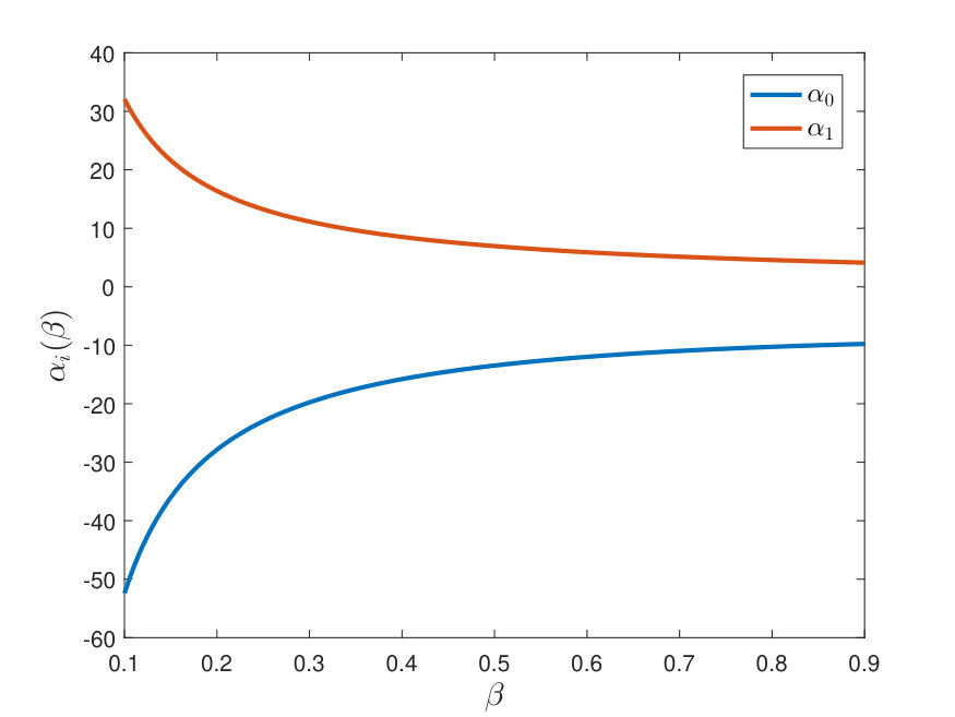 Figure 1
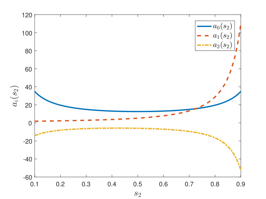 Figure 2
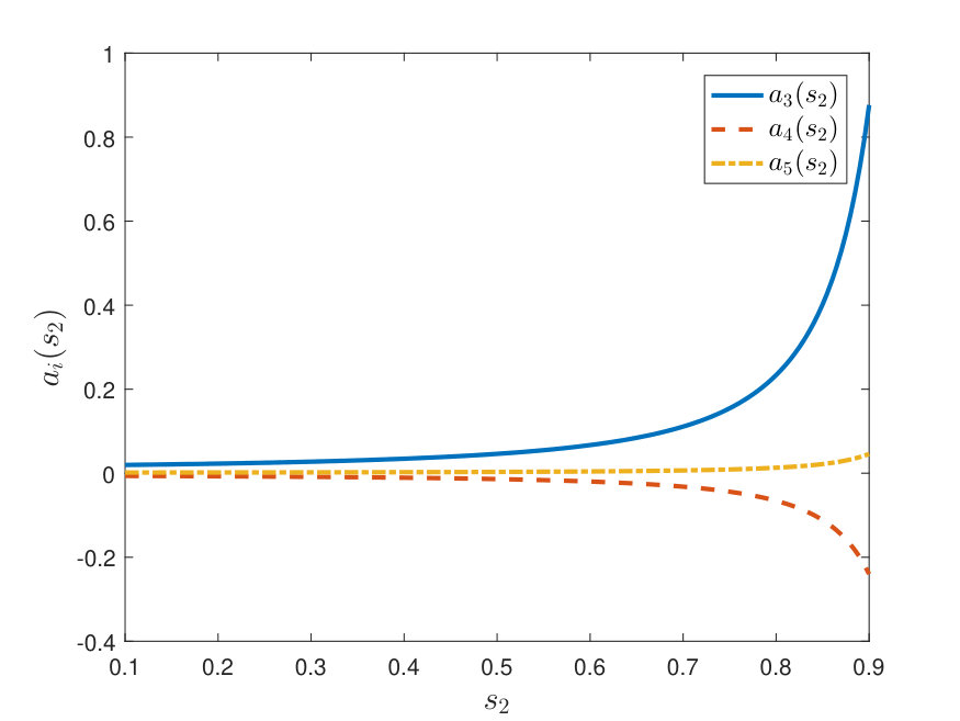 Figure 3
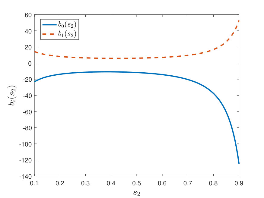 Figure 4
 Figure 5
 Figure 6
 Figure 7
 Figure 8
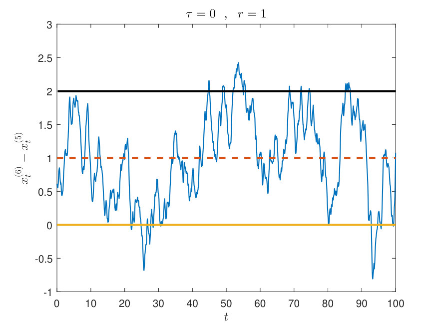 Figure 9
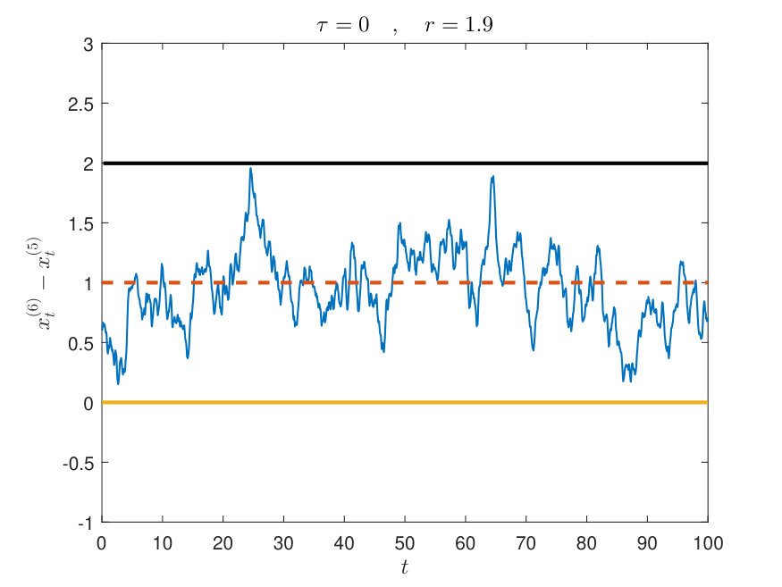 Figure 10
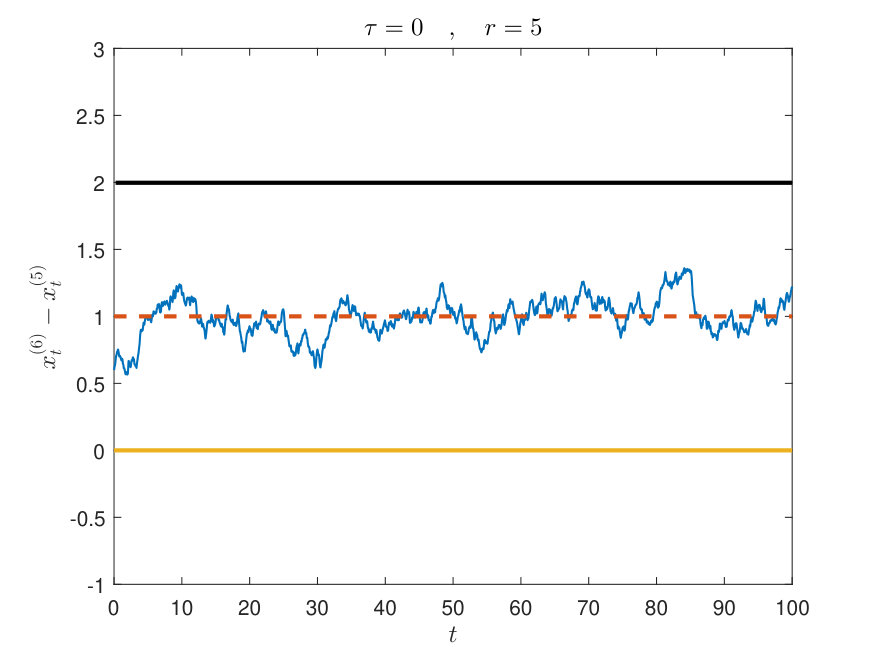 Figure 11
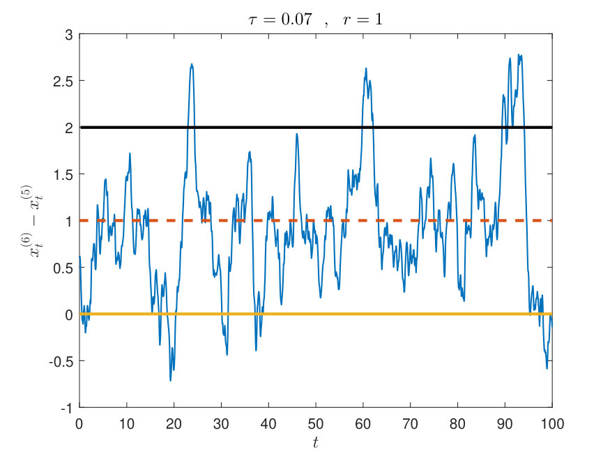 Figure 12
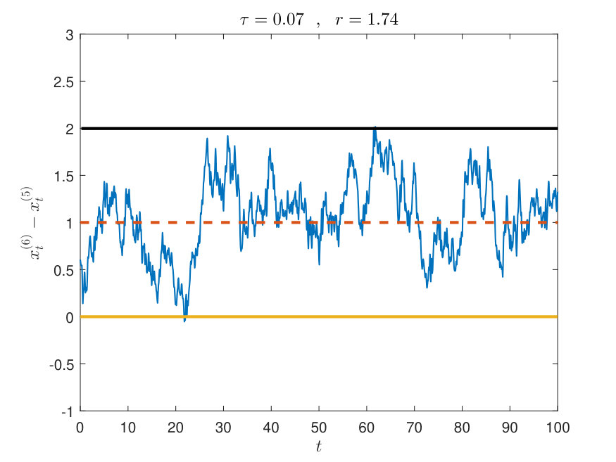 Figure 13
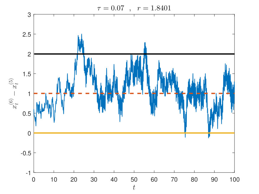 Figure 14
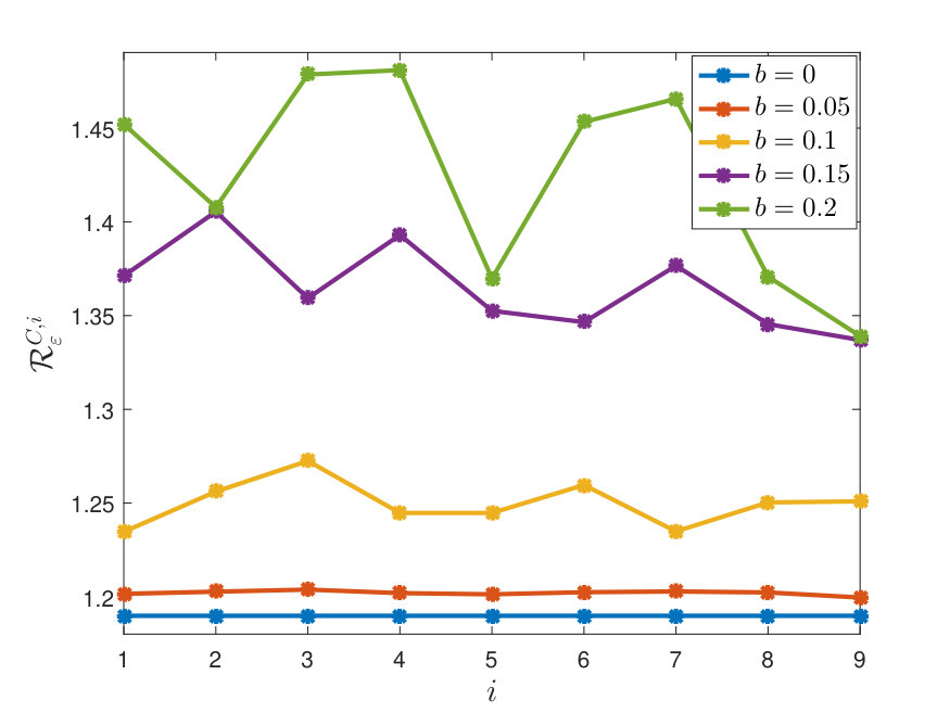 Figure 15
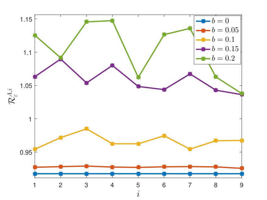 Figure 16
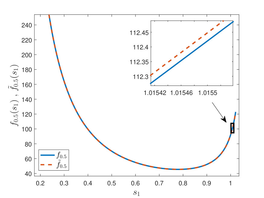 Figure 17
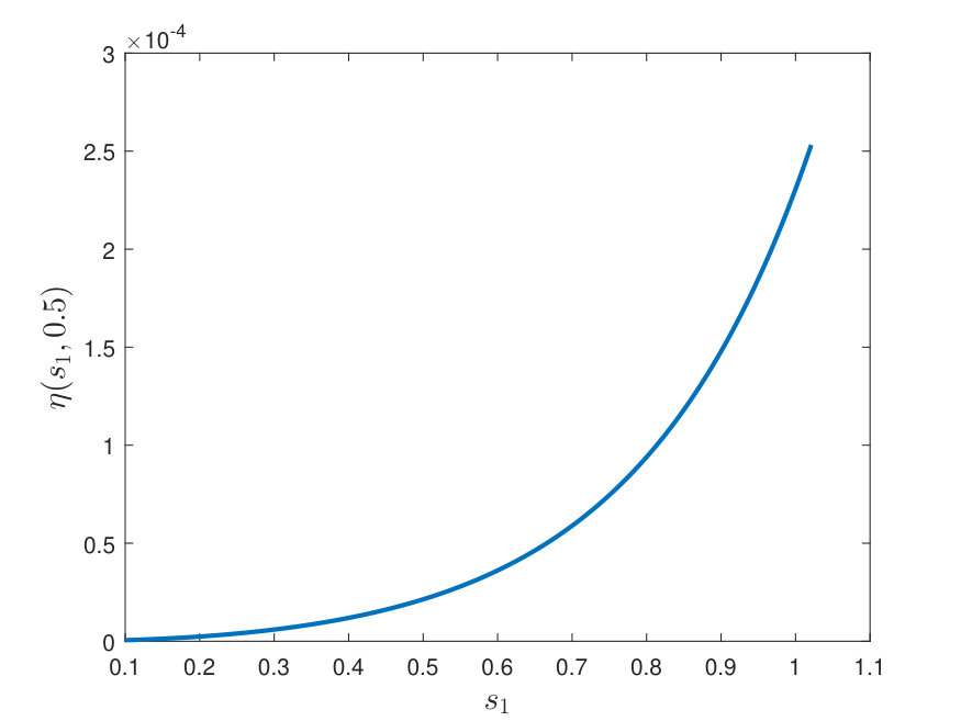 Figure 18
 Figure 19
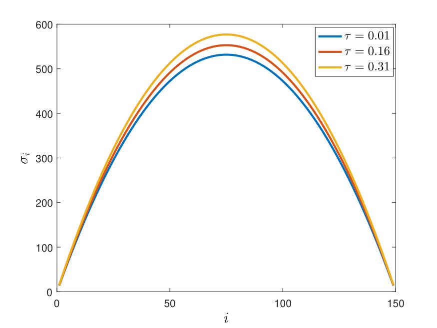 Figure 20
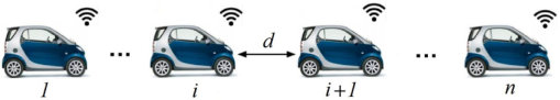 Figure 21
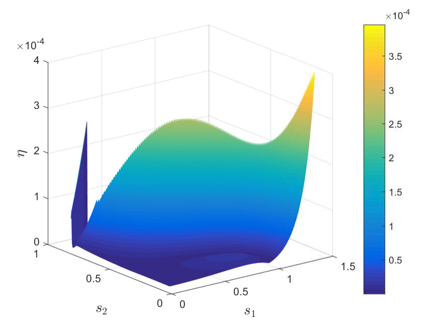 Figure 22
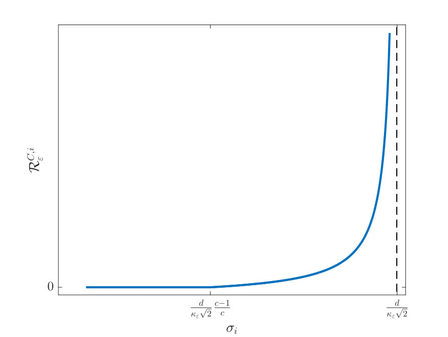 Figure 23
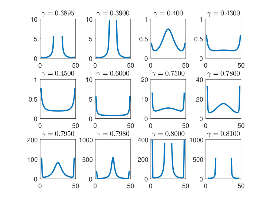 Figure 24
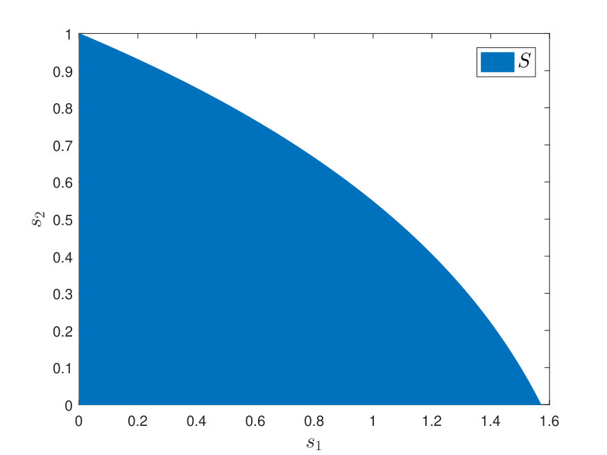 Figure 25
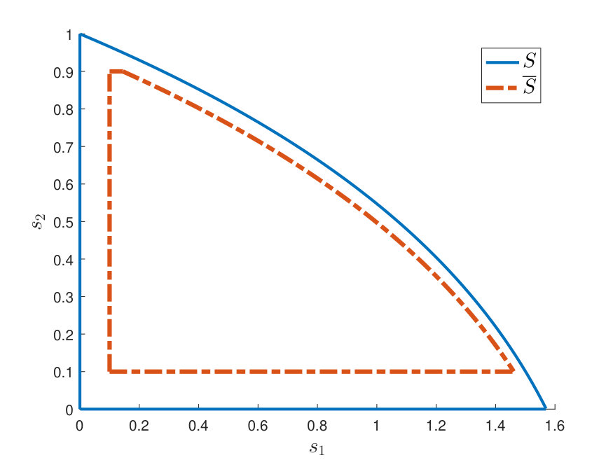 Figure 26
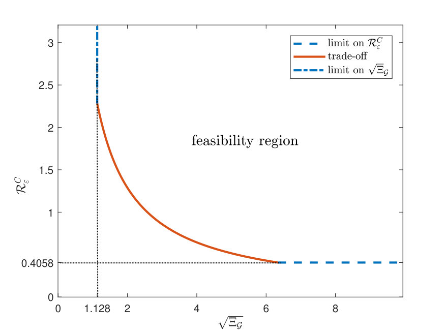 Figure 27
 Figure 28
Peer Reviews
No public reviews on file for this paper yet. If you reviewed it on a platform where reviews are public (OpenReview, ICLR, NeurIPS, ICML), you can paste yours below so the community can read it here.
Videos
No videos yet. Explain this paper in a talk, walkthrough, or lecture? Add one.
Risk of Collision and Detachment in Vehicle Platooning: Time–Delay–Induced Limitations and Trade–offs
(Extended Version)
Christoforos Somarakis, Yaser Ghaedsharaf, Nader Motee *This work is supported by NSF CAREER ECCS-1454022, AFOSR FA9550-19-1-0004 and ONR YIP N00014-16-1-2645C. Somarakis is with the System Sciences Lab, Palo Alto Research Center, Palo Alto, CA, 94304 [email protected]. Y. Ghaedsharaf and N. Motee are with the Department of Mechanical Engineering and Mechanics, Lehigh University, Bethlehem, PA, 18015, USA. {ghaedsharaf,motee}@lehigh.edu
Abstract
We quantify the value-at-risk of inter-vehicle collision and detachment for a class of platoons, which are governed by second-order dynamics in presence of communication time-delay and exogenous stochastic noise. Closed-form expressions for the risk measures are obtained as functions of Laplacian eigen-spectrum as well as their fine explicit approximations using rational polynomial functions. We quantify several hard limits and fundamental trade-offs among the risk measures, network connectivity, communication time-delay, and statistics of exogenous stochastic noise. Simultaneous presence of stochastic noise and time delay in a platoon imposes some idiosyncratic behavior risk of collision and detachment, for instance, weakening (improving) network connectivity may result in lower (higher) levels of risk. Furthermore, a thorough risk analysis is conducted for networks with specific graph topology. We support our theoretical findings via multiple simulations.
I Introduction
Networked control systems are often susceptible to external disturbances and onboard hardware limitations (e.g. communication time-delay, limited computational power and battery life). Notable examples of such networks include platoon of autonomous vehicles, synchronous power networks with integrated renewable sources, water supply networks, transportation networks, and inter-dependent financial systems [1, 2, 3, 4, 5]. Exogenous disturbances usually steer trajectory of a system away from the target equilibrium and potentially into undesirable modes of operation. The situation becomes even more challenging when the unperturbed network consists of several interconnected subsystems, where the troublesome effects of noise propagate and get amplified across the network. Moreover, inherent limitations on the communication layer (e.g., time-delay, receiver and transmitter noise) may also exacerbate the effect of noise and deteriorate the overall performance of the network. One of the main engineering challenges is to design robust dynamical networks that damp, if not reject, undesirable network-wide effects of disturbance and communication time-delay.
In this paper, we consider platoons vehicles that exchange information over a time-invariant communication network. The platooning problem is a simple, yet rich, benchmark to study autonomy in robotic networks using their second- or third-order state-space models [6, 7, 8, 9, 10]. We assume vehicle dynamics to be represented by a double control integrator. Also vehicles are capable of receiving, transmitting and processing data to update their own state, according to a second-order consensus protocol. Stemming from real-world applications, vehicles suffer from non-negligible communication time-delays due to deficiencies of existing hardware modules. It is assumed that all vehicles use identical hardware modules and, as a result, they all experience a uniform (identical) time-delay. In addition, the effects of uncertain surrounding environment on vehicles are modeled and incorporated into our network model via additive independent Gaussian force noises.
The global objective of platooning is to guarantee the following two group behaviors in steady-state: (i) pair-wise difference between position variables converges to a prescribed distance, and (ii) the platoon of agents attain the same constant velocity. This is illustrated in Figure 1. We identify two types of undesirable events, also referred to as systemic events. It is crucial to identify a systemic event where at least two consecutive vehicles collide and calculate its probability. We recall that a near-hit-region for two consecutive vehicles in platoon is an unsafe region in the state space of trajectories, as once there, vehicles may collide. This local event may interrupt the platoon and render the state of the entire network to unsafe regions in the state space. Similarly, no two consecutive vehicles may stand off too remotely, as once there, the communication graph of the platoon may be. Identifying and accounting for such events becomes substantially challenging when platoon is subject to exogenous stochastic noise and communication time-delay.
Related Literature: Norm induced performance and robustness measures have been widely studied in the context of robust control [11]. Reference [12] gives an overview and a brief history of risk-sensitive stochastic optimal control and surveys various approaches to controller design as well as their relationships among each other. The control objective, in this context, is to synthesize a controller with satisfactory levels of performance in the presence of disturbances. These methods face severe shortcomings when they are applied to stochastic dynamical networks. The resulting controllers usually require all-to-all communication and do not respect topology of the underlying communication layer [13]. Moreover, these controller design methods do not scale with network size.
The –norm has been recently utilized as a measure of performance and coherency for linear consensus networks (see [1, 14, 15, 16, 8] and references therein). One of the main advantages of using –norm is its elegant representation in terms of Laplacian spectrum that makes development of tractable and scalable network design algorithms possible [17]. An interesting interpretation of the norm, in the context of platooning, is that it quantifies the ability of the entire platoon to withstand the effect of exogenous noise and remain a rigid body [1]. The effects of time-delay in consensus networks have been investigated in various disciplines such as, to name only a few, traffic networks, flocking, distributed optimal control design [6, 1, 18, 19, 20, 21, 22, 23]. These works are mainly concerned with the problem of stability. Performance analysis and design of time-delay linear consensus networks using -norm is recently studied in [8, 15, 24, 25, 26, 27].
The –norm is an example of norms of Hardy-Schatten type. These systemic metrics quantify macroscopic features of networks. For instance, in consensus networks, –norm measures coherency [1] and –norm quantifies global connectivity [17]. However, these measures cannot scrutinize microscopic behaviors of networks. The focus of this paper is to inspect risk of inter-vehicle collision or detachment in the platoon of vehicles. We build upon existing notions of risk that are widely used in the context of financial systems [28, 29]. In its rudimentary form, risk serves as a surrogate for uncertainty in stochastic models [30]. We utilize the notion of value-at-risk to measure the extend and occurrence of a random undesirable event, with a certain confidence level, over a specified time period.
Our Contributions: Building upon our recent works on first order consensus systems [31, 32, 33], we investigate aspects of fragility in the platooning model from a systemic risk perspective. In Section V, the value-at-risk measure is quantified to determine safety margins for the following two types of undesirable events: (i) inter-vehicle collision, and (ii) inter-vehicle detachment. For a single collision or detachment event, we obtain a closed-form expression of risk in terms of Laplacian spectrum in Section VI. In Section VII, tight lower and upper bounds in terms of risk of individual events are provided for risk of multiple (joint) events. We outline the computational difficulties in deriving explicit expressions for the risk measures in Section IX and provide a tractable method for their approximation using rational functions. In Section VIII, we prove that fundamental limits and tradeoffs emerge on the best achievable levels of risk, which are solely due to the presence of exogenous noise and communication time-delay. Furthermore, we show that strengthening (weakening) network connectivity results in higher (lower) levels of risk of inter-vehicle collision and detachment. Finally, in Section X, we apply our approximate formulas to calculate risk of platoons with complete, path, and cyclic communication topologies and show how to identify high-risk vehicles in such networks. The paper concludes with Section XI of simulation examples that outline the theoretical results and Appendix sections with proofs of technical results.
Risk analysis of the platooning problem in this paper differs in almost every building block from our earlier works on first-order linear consensus networks [31, 32, 33]. First, the time-delayed second-order linear consensus networks are inherently more perplexed. Therefore, the stability conditions, that serve as cornerstone of our results, require fundamentally different analytic approach. Second, the nature of systemic events are different, which in turn, result in new risk formulas that do not lend themselves to explicit expressions in terms of Laplacian spectrum. The present paper is an outgrowth [34] in several different aspects. First, we extend our risk analysis to inter-vehicle detachment events as well as multiple systemic events. We propose a tractable rational function approximation scheme for evaluation of risk. Furthermore, we examine special communication topologies and present extra simulation examples. The manuscript also contains detailed proofs of all our technical results.
II Preliminaries
The -dimensional Euclidean space with elements is denoted by , where will denote the positive orthant of . We denote the vector of all ones by . For every , we write if and only if . The set of standard Euclidean basis for is represented by . The vector or induced matrix -norms are represented by . The vector of all ones is denoted by .
Algebraic Graph Theory: A weighted graph is defined by , where is the set of nodes, is the set of links (edges), and is the weight function that assigns a non-negative number to every link. Two nodes are directly connected if and only if . The set of nodes adjacent to constitutes the neighborhood of node that is denoted by \mathcal{N}_{i}=\big{\{}j\in\mathcal{V}~{}\big{|}~{}(i,j)\in\mathcal{E}\big{\}}.
Assumption 1**.**
Every graph in the paper is connected. In addition for every , the following properties hold:
(i) if and only if ;
(ii) , i.e., links are undirected;
(iii) , i.e., links are simple.
The Laplacian matrix of is a matrix with elements
[TABLE]
where . Laplacian matrix of a graph is symmetric and positive semi-definite. Assumption 1 implies that the smallest Laplacian eigenvalue is zero with algebraic multiplicity one. The spectrum of can be ordered as
[TABLE]
The eigenvector of corresponding to is denoted by . By letting , it follows that with . We normalize the Laplacian eigenvectors such that becomes an orthogonal matrix, i.e., with . The total effective resistance of is a popular metric of connectivity [35] that is characterized as [36]
[TABLE]
The smaller the value of , the stronger the connectivity of .
Probability Theory: Let be the set of all -valued random vectors \mathbf{z}=\big{[}z^{(1)},\dots,z^{(q)}\big{]}^{T} of a probability space with finite second moments. A normal random variable with mean value and covariance matrix is represented by . The error function is
[TABLE]
which is invertible on its range. The complementary error function is . Formulation of stochastic differential equations, we employ standard notation for stochastic differentials111This formalism will also be retained for deterministic differentials..
III Problem Formulation
Suppose that a finite number of vehicles form a platoon along the horizontal axis. Vehicles are labeled in descending order, where the ’th vehicle is assumed to be the leader. The ’th vehicle’s state is determined by , where is the position and is the velocity of vehicle . The ’th vehicle’s state evolves in time according to the following stochastic differential equation
[TABLE]
where is the control input at time . The terms represent white noise generators affecting dynamics of the vehicle and models the uncertainty diffused in the system. It is assumed that noise acts on every vehicle additively and independently from the other vehicles’ noises. The noise magnitude is represented through diffusion , assumed identical for all . The control objectives for the platoon are to guarantee the following two global behaviors: (i) pair-wise difference between position variables of every two consecutive vehicles converges to zero; and (ii) the platoon of vehicles attain the same constant velocity in steady state. It is known that the following feedback control law can achieve these objectives
[TABLE]
Let us denote the communication graph by , where , iff , and for all . The feedback gains are designed so that the resulting communication graph with Laplacian matrix (1) satisfies Assumption 1. The constant is the communication time-delay. The first term in (5) guarantees the control objective (i). The second term in (5) guarantees the control objective (ii) and stabilizes the relative position of vehicles and around the distance . The control parameter balances the effect of the relative positions and velocities. Following the scenario described in Figure 1, we select for some parameter and all . The target distance between vehicles and becomes . Let us define the vector of positions, velocities, and noise inputs as , , and , respectively222The stochastic process with \boldsymbol{\xi}_{t}=\big{[}\xi_{t}^{(1)},\dots,\xi_{t}^{(q)}\big{]}^{T}\in\mathcal{L}^{2}(\mathbb{R}^{q}) denotes an -valued Brownian motion.. By applying the feedback control law (5) to (4) and denoting , the closed-loop dynamics can be cast as the following initial value problem:
[TABLE]
for all and given deterministic initial functions over . Standard results in the theory of stochastic functional differential equations [37] guarantee that (6) generates a well-posed stochastic process .
The problem is to quantify risk of systemic events as a function of communication graph , time-delay, and statistics of noise. The systemic events are undesirable events that lead to greater (negative) impact on the global behavior of the platoon. We consider two types of systemic events: inter-vehicle collision, where two successive vehicles get too close to each other, and inter-vehicle detachment, where two successive vehicles distance themselves too far from their target distance and lose connectivity333This is practically relevant as vehicles are usually equipped with communication modules with limited range..
IV Stability and Solution Statistics
We investigate stability of the unperturbed closed-loop network, i.e., when in (6). Then, we analyze the statistical properties of the solution of (6) when .
Definition 1**.**
The solution of network (6) converges to a platoon if
[TABLE]
for all and all initial functions over .
Decomposition of offers a useful transformation
[TABLE]
In this new coordinates, (6) transforms to
[TABLE]
IV-A Exponential Stability of the Unperturbed System
Consider the set
[TABLE]
It is noted that so long as there equation is true for a unique . Figure 3 illustrates geometry of .
Theorem 1**.**
The solution of network (6) with converges to a platoon if and only if
[TABLE]
Remark 1**.**
Theorem 1 also holds for . In the absence of time-delay, the decomposed characteristic polynomial of (7) reads with roots that both lie on the left half plane. We note however that conclusion of Theorem 1 seizes to hold when . In this case, vehicles will align their velocities but not their relative distances.
Remark 2**.**
Stability properties of noise-free system (6) were previously analyzed in [22]. Theorem 1 proposes conditions that are more suitable for the analysis to follow.
IV-B Steady-State Statistics of Positions and Velocities
System (7) can be decomposed into two-dimensional subsystems with state variables \big{[}z_{t}^{(i)},\upsilon_{t}^{(i)}\big{]}^{T} for . We apply the variation of parameters formula for Itô calculus [37] to express the solution of the decoupled subsystems
[TABLE]
According to the conditions of Theorem 1, the principal solution of the unperturbed system, see (27), is exponentially decaying (stable) with respect to the consensus equilibrium. The vector depends on the initial functions and B_{i}=\big{[}\mathbf{0}_{1\times n}\hskip 1.42271pt,\hskip 1.42271pt\mathbf{q}_{i}^{T}\big{]}^{T}. For each , the process \big{\{}\big{[}z^{(i)}_{t},\upsilon^{(i)}_{t}\big{]}^{T}\big{\}}_{t\geq-\tau} is well-defined and as it converges, in distribution, to the bi-variate normal \mathcal{N}\big{(}\mathbf{0},\Sigma_{\infty}^{(i)}\big{)} with covariance
[TABLE]
The steady-state statistics, which are free from the transient effects of initial functions, carry the effects of the persistent network features, i.e., the communication topology, time-delay, and statistics of the exogenous uncertainties. Explicit calculation of is neither feasible nor useful. We are interested in studying events that are related to the relative distance between vehicles. We are thus only concerned with the marginal statistics of the above system, rather than the full state, i.e., the statistics of for all .
Lemma 1**.**
Suppose that conditions of Theorem 1 hold. Then,
[TABLE]
for all , where is defined as
[TABLE]
The result implies that \big{\{}\overline{z}^{(i)}\big{\}}_{i\in\{1,\dots,n-1\}}\in\mathcal{L}^{2}(\mathbb{R}) if and only if . The function is well-defined in the stability region , however, it cannot be calculated in an explicit form. To address this challenge, we propose in Section IX an efficient rational approximation of function .
V Value-At-Risk Measures
The standard deviation of a random variable in is one the common ways to quantify the uncertainty level encapsulated in that random variable. The notion of risk provides a more comprehensive and meticulous way to measure uncertainty in a random variable. Risk measures are defined either in terms of moments of a random variable or its distribution [30, 38]. In this work, we focus on the latter type of risk, known as value-at-risk measures444For moment-based risk analysis of a class of linear dynamical networks, we refer to [33] for more details.. These risk measures quantify the manner with which the uncertainty, nested in a random variable, steers its realization close to some undesirable range of values. Let us denote the set of undesirable values, which is also referred to as the set of systemic events, by . Then, the higher the risk on a random variable, the more likely that random variable will approach .
Definition 2**.**
Let be a probability space, and . The set of systemic events of is \big{\{}\omega\in\Omega~{}|~{}y(\omega)\in U\big{\}}\in\mathcal{F}.
We will evaluate the risk of \big{\{}\omega\in\Omega~{}|~{}y(\omega)\in U\big{\}} leveraging the distribution of . The idea is to construct a set structure to measure the distance of from . Then, the risk of systemic events for will be defined on the basis of this structure.
V-A Value-at-Risk of Scalar Events
Suppose that it is desirable for random variable to stay away from the set . Let us consider a collection of super-sets of with the following properties:
- ()
when 2. ()
for any sequence with property .
The collection can be further shaped to cover a suitable vicinity of . This vicinity plays the role of an alarm zone and yields high risk indexes as approaches . For some specific , the occurrence of \big{\{}y\in U_{\delta}\big{\}} signifies how close can get to in probability. The idea is implemented with the use of quantile functions on the systemic events of . For a given parameter , the risk measure is defined by
[TABLE]
The number is the cut-off value that characterizes the level of confidence on the systemic events. The smaller its value, the higher the confidence of the index . Let us elaborate and interpret what typical values of imply. The case signifies that the probability of observing dangerously close to is less than . We have iff for some (in fact, ) with probability greater than . The extreme case means that the event that is to be found in is assigned a probability greater than . In addition to several interesting properties (see for instance [32, 38, 30]), the risk index (11) is non-increasing with .
Proposition 1**.**
Let and consider the set of undesirable values together with the collection of supersets that satisfy properties and . Then,
[TABLE]
The motivation for risk in terms of quantile functions (11) emanates from the fact that (6) admits stochastic dynamics with random variables in with tractable distributions. It is then desirable to monitor the stochastic volatility of desired observables w.r.t. to a specific subset of .
V-B Value-at-Risk of Vector of Events
For the case of random vectors , we first extend the notion of super-sets by considering the product set , where . Similar to the scalar case, each sequence \big{\{}U_{\delta_{i}}\big{\}}_{\delta_{i}\in\operatorname{\mathbb{R}}_{+}} is assumed to satisfy properties and . The multi-dimensional extension of Definition 2 includes systemic events constructed through combination of set operations. One scenario, for example, is through the union operation
[TABLE]
In this case, the associated risk measure becomes
[TABLE]
A moment of reflection on (12) reveals that their calculation requires treating multivariable distributions. Unfortunately, these are rarely expressed in closed form. A computationally efficient surrogate is the vector of scalar risks, defined as
[TABLE]
where
[TABLE]
for . The vector is a collection of the scalar risk measures based on the individual distributions of for . In section VII, we revisit this part by formulating several vector of systemic events that are of interest to risk analysis of the platooning problem. Furthermore, we investigate their relations with the more computationally tractable vector .
VI Risk Of Single Systemic Events In The Platoon
We consider systemic events of inter-vehicle collision and detachment between two successive vehicles in the platoon. Let us represent the relative position of vehicles and in steady-state by the random variable
[TABLE]
where its statistics can be directly inferred from those of .
Theorem 2**.**
Let the conditions of Theorem 1 hold. Then, the steady-state solution of (6) satisfies
[TABLE]
with
[TABLE]
for and as in (10).
We utilize the result of this theorem to calculate risk of inter-vehicle collision and detachment for two successive vehicles.
VI-A Inter-Vehicle Collision
In absence of noise and under the conditions of Theorem 1, the steady-state distance between two successive vehicles satisfy . The differential term forces to fluctuate around . Vehicles and experience a collision if at some . If , then the collision has already occurred at some time prior to . When is positive, but close to zero, this will be an alert for a near collision. Let us define to be the zone of potential collisions, where parameter models the fluctuation magnitude and determines the upper endpoint of the collision set. For example, the collision set is , which allows no tolerance for any deviation from the target distance between the two consecutive vehicles. For , the collision set implies that there is no risk involved with the relative distance between two consecutive vehicles being in . In summary, we can use the steady-steady statistics and infer whether vehicles and have already collided or are dangerously close to each other if or , respectively. The union of the two disjoint sets define the family of parameterized events
[TABLE]
for . It is straightforward to verify that the collection satisfies properties and . Then, the associated risk measure is defined as555We read as the risk of collision between vehicles and with confidence level . Similar notation is used for detachment risk.
[TABLE]
for confidence level . In other words, is the safety margin below which the likelihood of a past collision or a new one to be developed is less than . The larger the value of risk, the higher the probability of the two vehicles being vulnerable to a collision.
Theorem 3**.**
Suppose that the conditions of Theorem 1 hold. For every , the risk of inter-vehicle collision is
[TABLE]
where is as in Theorem 2 and .
The two extreme values of are self-explanatory. In the unperturbed case, there is no risk of collision in the long run because asymptotic platooning is achieved exponentially fast. In this case, we have , which implies . When noise is present, we have . For large enough, vehicles lie far away from each other in expectation. Hence vehicle collision is unlikely to occur. Finally, when the standard deviation exceeds an -dependent cut-off, the value of risk is in the following sense: collision cannot be avoided with probability higher than for this range of ’s. The curve of is graphically illustrated in Fig. 4.
VI-B Inter-Vehicle Detachment
Cohesive motion in convoys of vehicles implies aligned traveling of agents within prescribed distance. For platooning ensembles of Fig. 1 any two successive vehicles that steered too distant from each other may trigger undesirable phenomena. A case-study that resonates with the geometry of Fig. 1 is this: In practice, vehicles are equipped with onboard finite-range communication modules. The ’th vehicle can establish reliable communication with those vehicles whose positions lie in range , where is the communication range. Thus, a condition like is necessary to guarantee existence of a reliable communication topology that guarantees reliable transmission of data in accordance to Assumption 1. Without loss of generality, let us take
[TABLE]
for some parameter . In the presence of stochastic noise, it is likely that two successive vehicles move further away from each other beyond and into dangerous communication status. Detachment between vehicles and occurs when their relative position exceeds . It is said that vehicles and are dangerously close to lose communication and experience detachment when takes values in \big{[}ad-\frac{1}{h},ad\big{]} for some design parameter . Parameter plays the same role as parameter in the inter-vehicle collision scenario: the higher the value of , the narrower the length of the alarm zone prior to experiencing detachment. Let us define the family of parameterized events
[TABLE]
for . Similar to the collision super-sets, the collection satisfies properties and . The value-at-risk of detachment between vehicles and is defined as
[TABLE]
for fixed confidence level . Following the same steps as in the proof of Theorem 3, the closed-form expressions for the risk of platoon detachment is given by
[TABLE]
where , and is as in Theorem 2. Both collision and detachment scenarios are illustrated in Fig. 5.
VII Risk Of Multiple Systemic Events In The Platoon
We generalize results of the previous section by considering multiple collision and detachment events that involve more than two vehicles and may happen simultaneously. The idea is to define proper super-sets for random vectors \mathbf{y}=\big{[}y^{(1)},\dots,y^{(q)}\big{]}^{T}, where for . In the following, several scenarios are considered.
By constructing the full conjunction of the individual events discussed in Section VI, we can formulate risk of simultaneous collision and detachment between some pairs of successive vehicles throughout the platoon via
[TABLE]
The risk of simultaneous collision and detachment across the platoon is measured by
[TABLE]
The calculation of either (18) or (19) in closed-form is mathematically intractable as it requires working with multi-variable normal random variables. Since obtaining an explicit expressions is not feasible, we rely on first-order approximations using the vector of individual surrogates as in (13). Let us define the vectors of individual risks for collision and detachment as
[TABLE]
respectively.
Theorem 4**.**
Suppose that conditions of Theorem 1 hold. The risk of simultaneous collision and detachment of all vehicles satisfies
[TABLE]
where
[TABLE]
where is replaced by either or , and the risk of simultaneous collision and detachment of some of the vehicles satisfy
[TABLE]
where
[TABLE]
with being either or .
As it is discussed in the Appendix, this result relies on the Boole-Fréchet inequalities. These inequalities are the best possible estimates on unions and intersections of events for which nothing is known other than the probabilities of the corresponding individual events [39]. We remark that, unlike the case of global union of events in Theorem 4, there is no non-trivial lower limit for the risk of global joint events. Despite their elegance, Boole-Fréchet inequalities fail to provide non-trivial lower bounds for the type of joint risk events. This point is elaborated in the Appendix.
One can define more general scenarios by grouping the elements of into classes of interest. Let be a partition of the set into mutually disjoint subsets , where denotes the cardinality of . It follows that . This labeling classifies the elements of into groups. This notation allows to formulate the following class of risk measures
[TABLE]
and
[TABLE]
in which is either or . The risk measure (19) is a special case of (21) when , where (21) quantifies risk of at least one event in every group of the partition will experience a systemic event. Similarly, (18) is a special case of (22), where (22) measures likelihood of all members of at least one of the groups in the partition experiences a systemic event. The results of Theorem 4 and Proposition 1 can be combined to obtain bounds for (21) and (22) in terms of vector (20). The results of this section allow us to design low risk platoons by formulating multi-objective optimization problems based on vectors of individual risk measures.
VIII Fundamental Limits and Trade-Offs
An engineer has almost no control over the communication time-delay and exogenous disturbances. In such situations, one can design optimal communication topologies to minimize the disruptive effect of such imperfections. Our goal is to explore inherent shortcomings in network design when the effects of neither noise nor time-delay can be neglected666Discussion in this and the following sections is focused on risk of inter-vehicle collision. Results on detachment can be derived in a similar fashion..
Lemma 2**.**
The marginal standard deviations , as in Theorem 2, satisfy the lower bound
[TABLE]
for , where .
This result reveals that the variance of attains a hard lower bound that only depends on the strength of the diffusion and the time-delay .
Theorem 5**.**
There is an inherent fundamental limit on the best achievable values of risk of inter-vehicle collision in the platoon that is given by
[TABLE]
According to this result, the systemic risk measure attains the trivial lower limit zero when is less than or equal to the critical value . If lies in a specific set of values, the risk of collision can be minimized as a function of communication topology. On the other extreme, risk of inter-vehicle collision becomes infinite (i.e., collision becomes inevidable) if exceeds a safety cut-off value. In fact, we can characterize an inevitability condition as follows: the risk of collision between two consecutive vehicles is infinite for all platoons, independent of their communication topology, if
[TABLE]
for all . The risk can be reduced by minimizing the marginal standard deviations up to a limit, which is characterized by Lemma 2, by adjusting the platoon’s control parameters (i.e., feedback gains and ). According to Theorem 3 and Lemma 2, the Laplacian spectrum of a platoon with minimal risk must satisfy
[TABLE]
where and are determined through
[TABLE]
Therefore, the optimal communication topology is a complete graph with link weights for all .
Optimal network topology as described above is far from ideal in real-world situations. Given an arbitrary (sub-optimal) network, synthesis objective regards developing formal methods to attain safe vehicle interactions. In this setting, safe is interpreted as the control topology that mitigates risk of systemic events. To this end, we recall that network synthesis is conducted via adding new feedback loops (coupling links), sparsifying, or adjusting the exiting feedback gains. Every such operation impacts the eigen-spectrum of graph laplacian , and this has immediate consequence on systemic risk measures . In the remainder of this section we report the existence of a counter-intuitive trade-off between network connectivity and risk of inter-vehicle collision. The measure of network connectivity, already introduced in §IV, is the effective graph resistance . The next result is an interesting delay-induced fundamental limitation in close spirit to Theorem 5.
Theorem 6**.**
For given control parameter and such that , the communication connectivity, which is specified using the total effective resistance (3), cannot be improved beyond some certain threshold according to inequality
[TABLE]
where \vartheta~{}:~{}(0,1)\rightarrow\big{(}0,\frac{\pi}{2}\big{)} is defined by
[TABLE]
with and .
The smallest lower bound for (23) is achieved when , which in that case (23) becomes
[TABLE]
The main advantage of , over other measures of connectivity (such as vertex/edge connectivity [40]) is that effective resistance applies equally well to weighted symmetric graphs as well as to topological (unweighted) graphs. Moreover it attains an elegant spectral representation that favors the comparison with risk expressions derived in Theorem 3. Going beyond hard limits, we show that fundamental trade-offs emerge between risk and network connectivity. These trade-offs explain that for a non-trivial range of feedback gains, , improving connectivity, which results in decreasing , leads to higher levels of systemic risk. For a rigorous exposition of our results, we need to employ some new notations. Let us define
[TABLE]
for every , where is given by (10) and by (24), as well as
[TABLE]
in which is the fundamental limit of as in Lemma 2. We also define the sequences with elements that are defined by
[TABLE]
Theorem 7**.**
Suppose that the conditions of Theorem 3 hold. For , if , then and a fundamental trade-off between the best achievable levels of collision risk and communication connectivity emerges as follows
[TABLE]
Theorem 7 asserts that, for a non-trivial range of network parameters, the only way to maintain a safer (low-risk) network is through weakening the communication connectivity, e.g., by decreasing the feedback gains or sparsifying the communication graph. Equivalently, strengthening the connectivity, e.g., by increasing the feedback gains or adding new feedback loops or links, increases the risk of collision (and detachment) between the vehicles. The intrinsic trade-off between risk and communication connectivity is due to the combined effect of time-delay and noise.
We conclude this section by highlighting that all the fundamental limits and trade-offs disappears when time-delay is absent, i.e., strengthening the connectivity among the vehicles reduces chances of witnessing collision events in the platoon.
IX Approximation Formulas For Risk
Calculating explicit closed-form solutions for delay differential equations is almost impossible. This is also true for the delay model of platoon (6) and its transition matrix . It was shown that the covariance matrix depends on as in (9). In fact, obtaining an explicit expression for the solution of the unperturbed platoon heavily depends on the form of function as in (10). Although has a closed-form, it does not admit an explicit form. Consequently, the formulas in (15) and (17) are expressed in terms of improper integrals. This induces a computational burden that quickly becomes an issue as the number of vehicles in the platoon increases. Thus, it is desirable to find efficient approximations of over its domain in order to reduce computational complexity of our proposed methodology. Our investigation reveals that the behavior of , depending on its parameters, is similar to some non-trivial rational function for which the existing conventional approximation techniques (e.g., Legendre polynomials) are proven to be inefficient. In the following, we first propose a rational approximation for along with its relative error bound. The details of our derivations can be found in Appendix A. Then, this approximation is applied to obtain an efficient approximation of the risk measures.
We recall that diverges on the boundary of for where meets its poles. On the -axis, over which and is finite, the dynamics of the unperturbed platoon seize to satisfy Definition 1. Thus, we will approximate in a compact subset of that excludes any pole or degeneracy. We adopt a compact subset of that is characterized by , where is the solution of for . This subset is depicted in Figure 7 along with . One can verify that is invertible for and it can be expressed as . For , we choose the following class of rational functions
[TABLE]
in which the enumerators
[TABLE]
are polynomials in with real-valued coefficients that exclusively depend on . Functions and can not be expressed in closed-forms. Some typical graphs of these functions are shown in Figures 8. Figure 11 depicts the exact function and the rational approximation for together with the associated relative error. The relative error function
[TABLE]
is plotted in Figure 9 for all . Our extensive numerical experiments verifies that Moreover, computational explorations suggest that contains the minimum value of . This is a significant indication in favor of utilizing as a computationally efficient surrogate in order to develop efficient algorithms for design of low-risk platoons.
In the final step, we utilize approximation (26) and arrive at a tight approximation of the risk measure , where
[TABLE]
provided for .
X Examples Of Communication Topologies
Using the results of the previous section, we obtain approximate closed-form expressions for the risk of systemic events in platoons with certain symmetric communication topologies. The marginal variance is evaluated for platoons with complete, path, and -cycle communication graphs with uniform feedback gains, i.e., . The eigenvalues and eigenvectors of these graphs can be obtained explicitly [35, 41]. We restrict our attention to calculation of the marginal standard deviation of the relative distance between two successive vehicles. Through our analysis, it is possible to calculate the value-at-risk measures of the collision and detachment events for a given confidence level and set of parameters and .
X-A The Complete Graph
The eigenvalues of a complete graph are: and for all . For , the marginal standard deviation for the complete graph topology is
[TABLE]
for all . Using this quantity, one can easily calculate the value-at-risk measures. The first plot from left in Figure 10 illustrates as a function of time-delay , number of vehicles, network parameters , , and . We conclude that for small time-delay, larger ensembles of vehicles experience lower risk. For large value of , it appears that the smaller the ensemble, the safer the platoon.
X-B The Path Graph
The path graph over nodes has edges of weight. The eigenvalue is \lambda_{j}=2k\big{(}1-\cos(\pi(j-1)/n)\big{)} with the corresponding eigenvectors and \mathbf{q}_{j}=\big{[}q_{j}^{(1)},\dots,q_{j}^{(n)}\big{]}^{T} with q_{j}^{(l)}=\sqrt{\frac{2}{n}}\cos\big{[}\frac{\pi(n-j+1)}{2n}(2l-1)\big{]} if . The marginal standard deviation is
[TABLE]
with w(j,i,n)=\sin^{2}\big{(}\frac{\pi(n-j+1)}{n}i\big{)}\sin^{2}\big{(}\frac{\pi(n-j+1)}{2n}\big{)}. Then, one can easily calculate the risk measures. The second plot in Figure 10 illustrates with respect to vehicle labels, where it is assumed that communication graph in all simulations is path with network parameters , , and . We conclude that the safest regions with lowest risk of collision or detachment are located in the two ends of the platoon. As we approach the center, the risk of collision or detachment will increase monotonically and reach its peak half way before it begins decreasing again. This implies that the vehicles in the middle of the platoon are more likely than the others to experience collision or detachment. It is observed that time-delay uniformly increases the risk across the platoon.
X-C The -Cycle Graph
A platoon with a -cycle communication graph is a network where each vehicle communicates with its -immediate neighbors. The corresponding Laplacian matrix is a special type of circulant matrices whose eigen-structure is discussed in [41] from where it can be shown that and with ([\mathbf{e}_{i+1}-\mathbf{e}_{i}]^{T}\mathbf{q}_{j})^{2}=\frac{2}{n}\big{(}1-\cos\big{(}\frac{2\pi}{n}\big{)}\big{)} for all . The marginal standard deviation of the distance between vehicles and is
[TABLE]
The third plot from left in Figure 10 is a graphic illustration of the marginal variance over a platoon with vehicles as a function of parameter . The network parameters are , , , and . For small value of , i.e., for loosely connected platoons, the marginal variance, which is identical for all vehicles, is large. As connectivity enhances by increasing , the platoon becomes less fragile to systemic events of collision and detachment. Finally, when approaches the limit value , i.e., the complete graph topology, the eigenvalues approach the boundary of and the platoon becomes unstable. The authors acknowledge that it is an unrealistic to have vehicles to communicate over a cycle graph as the first vehicle may not be able to communicate with the last. However, the -cyclic graphs serves as a nice approximation for the -path graph when is large enough. For , the -cycle graph resembles a graph where every vehicle communicates with its nearest neighbors from each side (front and behind).
XI Simulations
We discuss three case studies for platoons with dynamics governed by (6). First, we show that time-delay can steer a platoon to become more prone to risk and eventually instability. The second case study illustrates that, in the presence of time-delay, deviating from the optimal graph topology increases the risk of systemic events. Finally, the third case examines how spatial localization of communication may affect the risk measures.
XI-A Risk Behavior vs. Connectivity
We consider a platoon of vehicles. The desired distance is set to , the scale between position and velocity alignment to , and the drift coefficient of noise to . The other parameters are and for the collision events, and , for the network detachment events. The desired relative distance between two successive vehicles and is . The vehicles are in collision when and the vehicles have lost connectivity when . The objective is to guarantee that vehicles 6 and 5 will neither collide nor lose connectivity. The corresponding values of risk measures are
[TABLE]
Topology of the communication graph is generated randomly by ensuring Assumption 1 and all feedback gains are equally chosen to be . The first round of simulations assumes a platoon without time delay. For , it turns out that is greater than the critical values and that results in . By tuning up the feedback gain to , the risk measures become and , which are rather large, but finite. Increasing to yields and . This is to verify that in the absence of time-delay, the risk of systemic events becomes small as connectivity improves.
Next, we consider a platoon with time-delay and repeat our simulations for different values of the feedback gain . At , it turns out that . As we increase feedback gain up to , the risk measure decreases to and , before it starts to increase again. At , it goes back to . Examples of the relative distance between vehicles 6 and 5 are illustrated in Figure 15 over time interval seconds.
XI-B Random Perturbations in Optimal Graphs
In this case study, we investigate how deviation from an optimal graph topology affects the risk of collision and detachment by considering a platoon with vehicles. The network parameters are , , , and . For the collision events, we have set and a cut-off value . For the detachment events, we have set , , and a cut-off value . We recall from Section VIII that the optimal communication graph is the one with and for . An optimal graph for our example is the complete graph with identical link weights for all . We generate random perturbation of the optimal topology by substituting feedback gain with new feedback gain , where is a random variable that is uniformly distributed in . Figure 12 illustrates the value of the elements of vectors and for different values of parameter . We remark that the risk of collision qualitatively behaves similar to the risk of detachment, although we numerically verified that they are not proportional. In addition, the risk of detachment is significantly smaller for all values of due to the difference in the cut-off values.
XI-C Spatially Decaying Topologies
In this case, we consider geometric graphs where all-to-all communication is allowed by enforcing the range of connectivity to decrease with distance. This class of communication graphs is typical in wireless communication networks. Each vehicle broadcasts its message, where signal-to-noise ratio of the received signal by another vehicle decreases with distance between the two vehicles. We consider a platoon with vehicles with usual ascending labels from to . The receiver of the ’th vehicle collects the state information of the ’th vehicle with feedback gain for some . The exponent is the spatial decay index or localization parameter. For small values of , the network topology approximates a complete graph. As increases, the effective communication range of vehicles becomes more localized. For large enough values of that preserve connectivity, the communication topology resembles the path graph. In Figure 13, we illustrate for different exponents and observe various transition of the risk profile. For small , the graph is heavily connected, which combined with the effect of time-delay results in increased risk values. The high risk vehicles are the ones in the middle. As increases, connectivity decreases and the platoon experiences lower risk of collision. It is remarkably interesting that the vehicles in the middle become very safe. For larger values of , the communication network keeps losing connectivity and risk of systemic events becomes more evident. The more susceptible vehicles for are again the ones in the middle. As exceeds , the communication gets very localized. Since is large, poor connectivity makes the platoon susceptible to noise, leading to infinite value of risk for many pairs of vehicles.
XII Discussion
We focused on collision or detachment events between vehicles in a platoon, where each vehicle is modeled as a double integrator subject to exogenous noise. The ensemble is controlled via a distributed consensus feedback control law that suffers from communication time-delay. We developed a risk oriented framework to assess the possibility of some relevant systemic events. Our model, albeit simple, facilitates a rigorous analysis to the point of characterizing intrinsic interplay among the risk measures, network connectivity, time-delay, and statistics of the exogenous uncertainty. Our results are particularly useful to design low-risk platoons by optimizing topology of the underlying communication network. On the downside, we acknowledge a number of shortcomings that pose new challenges for future research.
We would like to point out that it is possible to study risk on more general models. Risk measures ask for distributional properties of stochastic processes (in our case, solutions of a stochastic differential equation). It is well-known that evolutionary densities of stochastic dynamical systems typically satisfy partial differential equations of Fokker-Planck type. This means that, at least in theory, it is feasible to evaluate risk of systemic events for a broad class of dynamical systems. There is, however, little hope for closed-form solutions such as the ones established in this work. Analysis may only be feasible on a case-by-case basis. Linearity helps us to leverage the Ornstein–Uhlenbeck type of processes with normal distributions. Risk analysis provides a solid framework to study the manner with which marginal variances that encapsulate features of the dynamical system (network topology, time-delay, noise) characterize systemic fragility as they project on the geometry of undesirable events.
An interesting extension is to consider network with heterogeneous delays. Uniform time-delay is from many aspects simplistic. However, heterogeneity of time-delay destroys symmetry. A dire consequence is that it becomes quite challenging to identify stability region i.e., a crucial step for risk analysis. Numerical methods can be employed to overcome this hurdle [42].
The two systemic events considered in this work are the event of vehicles collision and the event of vehicles detachment. Undesirable (unsafe) behavior is triggered when two successive vehicles are either too close or too far away. The questions that fell within our scopes were on characterizing the types of interactions that promote robustness with respect to collision or detachment when real-world deficiencies, such as disturbance and time-delay, are present. One future extension is to consider internal structure (e.g., engine dynamics) and non-trivial shapes of vehicles. It would be interesting to explore how vehicle dynamics integrate with network assimilated data and distributed control laws for motion coordination. To this end, we would like to mention one important feature of vehicle dynamics, which is omitted in this work. That is acceleration damping, i.e. a stabilizing state-feedback control term on the rate of change of velocity of vehicles that ensures finite speed of the ensemble. In addition, absolute feedback control methods are in many cases known to generally improve performance [1, 18]. It would be very interesting to test these control policies from a risk theory perspective.
A final future research direction that is worth mentioning is to develop efficient and scalable algorithms to design communication topologies for platoons by striking a balance among connectivity, performance, and risk of collision or detachment events.
Appendix A: Rational Approximation Of
The function in (10) plays an instrumental role in the actual calculation of risk. As it is not explicitly stated, we can approximate for and in a compact subset of , defined as:
[TABLE]
where and it is presented in Figure 7, together with . For , we will construct a rational approximation of . Our approach relies on ideas developed in [43].
Now, we see that for fixed the function attains a pole at of order 4 and a pole at of order 1. In fact, the collection of all poles is the curved boundary of . The zero poles lie along the vertical axis. For fixed we recall and consider the vector space spanned by the functions
[TABLE]
The inner product
[TABLE]
for any , will be used to generate an orthonormal basis of following the Gram-Schmidt process. We arrive at
[TABLE]
We introduce
[TABLE]
with the weights . From the orthonormalization process, are linear combinations of elements of . Thus we can write as
[TABLE]
for that generally depend on . The first two coefficients, and are illustrated in Figure 14. Numerical explorations show that attain constant values , , , , , .777The aforementioned coefficients appear to be approximately constant for a large range of values in . In fact they all turn to be non-constant with non-smooth behavior for values near to . We approximated with their average in . We can discard the terms , for being of negligible magnitude and this yields
[TABLE]
Elementary algebra yields
[TABLE]
where
[TABLE]
The accuracy of is validated numerically. The results are depicted in Figure 9. The maximum relative error is of order .
Appendix B: Proofs
Proof of Theorem 1.
The stability problem of (6) is directly related to the stability of (7), that for , decouples to
[TABLE]
for . We can now study the dynamics of (6), by looking at (27) for every , independently. The stability of the sub-system (27) is characterized through the location of the roots of the characteristic function
[TABLE]
For we apply Theorem 13.12 in [44], to conclude that all roots of lie in the left complex half plane iff the conditions on and hold. Standard results in the theory of delay differential equations [45] assure that as
[TABLE]
exponentially fast for all . Inverting the transformation, we observe that in the limit which in turn implies . On the other hand, x_{t}^{(i)}-x_{t}^{(j)}=d_{i}-d_{j}+\mathbf{\sum}_{l=1}^{n}(q_{il}-q_{jl}\big{)}z_{t}^{(l)}=d_{i}-d_{j}+\mathbf{\sum}_{l=2}^{n}(q_{il}-q_{jl}\big{)}z_{t}^{(l)} because . So as , for and thus . ∎
Proof of Theorem 1.
The spatial-related steady-state statistics of the sub-system , are obtained from the marginal distribution of
[TABLE]
where . Using Parseval’s identity we obtain a more convenient integral representation:
[TABLE]
where , is the input-output transfer function:
[TABLE]
and the complex conjugate of . Elementary algebra yields
[TABLE]
and so
[TABLE]
Changing variables to , we obtain
[TABLE]
∎
Proof of Proposition 1.
Assume . Then , where is the solution of the optimization problem
[TABLE]
Since , is a feasible solution of the optimization problem
[TABLE]
Therefore . Now, let and label for . By construction of , for . Now, implies . Then and thus \mathbb{P}\big{(}y\in U_{\delta_{2}}\big{)}<\mathbb{P}\big{(}y\in U_{\delta_{1}}\big{)}, concluding the proof. ∎
Proof of Theorem 2.
From Theorem 1 we have shown that the vector \boldsymbol{\psi}:=\big{[}z^{(1)}_{t},\upsilon_{t}^{(1)},\dots,z^{(n)}_{t},\upsilon_{t}^{(n)}\big{]}^{T} is normally distributed with covariance matrix
[TABLE]
by virtue of the form of matrices . We introduce the affine transformation for a matrix with the row of to be the canonical vector . The covariance matrix of is written as for the matrix
[TABLE]
From and for fixed , we can express the relative position of vehicles and as
[TABLE]
In view of Assumption 1 we have , we conclude that the latter is yet another affine tranformation of a multivariate normal distribution, from which we deduce that is normally distributed, with covariance matrix
[TABLE]
Take the limit and apply Theorem 1 to conclude. ∎
Proof of Theorem 3.
Observe that (14) is equivalent to
[TABLE]
Therefore, in addition to the case , is equivalent to
[TABLE]
The last inequality is equivalent to the mutually exclusive cases:
[TABLE]
The union of these two cases, covers the first branch of (15). On the other hand,
[TABLE]
which in turn is equivalent to \text{erf}\big{(}\frac{d}{\sigma_{i}\sqrt{2}}\big{)}\leq 1-2\varepsilon, where is the error function. For we can invert the error function and conclude
[TABLE]
For the third branch of , we observe that the infimum of in (29) is achieved at
[TABLE]
and a convenient representation of risk is
[TABLE]
∎
Proof of Theorem 4.
The proof relies on the Boole-Fréchet inequalities:888The proof of which can be found in [39].: Let the collection of -measurable events . Then,
[TABLE]
[TABLE]
These inequalities are the best possible probability estimates of the events or when nothing else is known, other than the individual probabilities . We will focus on global collision event risk as the steps on risk of global detachment are identical. Observe that (19), can be cast as the solution of the chance constraint optimization problem
[TABLE]
Consider the solutions of the scalar problems
[TABLE]
In view of the right hand-side of (30), \boldsymbol{\delta}^{+}=\big{(}\delta_{1}^{+},\dots,\delta_{n-1}^{+}\big{)} is, in fact, a feasible solution of (32)-(33) :
[TABLE]
This establishes the upper bound of . The lower bound of set is trivial. We proceed with the second pair, for which we remark that is the solution of the following constraint optimization problem
[TABLE]
On the other hand, we can consider the solutions of the scalar problems
[TABLE]
for , and such that . Using (30) we can show that is a feasible solution of (36)-(37). Indeed,
[TABLE]
. On the other hand, if is the optimal solution of (36)-(37), then
[TABLE]
by virtue of the left-hand side of (30). Consequently, solve
[TABLE]
concluding the proof of the theorem. ∎
Proof of Lemma 2.
At first, observe that for attains a minimum in the interior of . This is because attains a compact closure, and diverges on its boundary. By virtue of continuity attains a minimum in its interior, let be this minimum i.e., . This is a value that can be numerically approximated . Then for as in Theorem 2, we calculate:
[TABLE]
where \sum_{j=2}^{n}\big{(}[\mathbf{e}_{i+1}-\mathbf{e}_{i}]^{T}\mathbf{q}_{j}\big{)}^{2}=\sum_{j=1}^{n}\big{(}[\mathbf{e}_{i+1}-\mathbf{e}_{i}]^{T}\mathbf{q}_{j}\big{)}^{2}=||\mathbf{e}_{i+1}-\mathbf{e}_{i}||^{2} due to the orthogonality of the vectors . ∎
Proof of Theorem 5.
The result follows directly after combining Theorems 1, 3, and Lemma 2. ∎
Proof of Theorem 6.
The proof directly follows from the eigenvalue restrictions dictated by the region . Let . Then for to satisfy . In other words,
[TABLE]
Inverting the last equality we obtain the limit . For given such that the limits are reversed so as to . The last condition has to be satisfied for all non-zero eigenvalues of . The result then follows directly by elementary algebra. ∎
Proof of Theorem 7.
We will work the details for the systemic risk of vehicle collision only. Throughout the proof and for notation simplicity. The steps to derive of the second trade-off condition is identical. From Theorem 3 we have
[TABLE]
Both the enumerator and the denominator are positive. We will establish non-trivial lower bounds for the two expressions independently. We start with the enumerator . It is easy to see that its minimum is achieved at , and it is achievable provided that the hard limit from Theorem 5. Consequently, . We proceed with the term . Since we can express as a geometric sum
[TABLE]
Now,
[TABLE]
The first term of the sum above is bounded by . The term of the second infinite sum term is handled as follows:
[TABLE]
From the eigenvalue ordering (1) and the conditions of Theorem 1, we deduce for , . Then
[TABLE]
Summing over all the terms, we arrive at the lower bound for
[TABLE]
We take the square root on both sides to conclude. ∎
The reference list from the paper itself. Each links out to its DOI / PubMed record.
- 1[1] B. Bamieh, M. Jovanović, P. Mitra, and S. Patterson, “Coherence in large-scale networks: Dimension-dependent limitations of local feedback,” Automatic Control, IEEE Transactions on , vol. 57, no. 9, pp. 2235 –2249, Sept. 2012.
- 2[2] F. Dörfler and F. Bullo, “Synchronization and transient stability in power networks and nonuniform kuramoto oscillators,” SIAM Journal on Control and Optimization , vol. 50, no. 3, pp. 1616–1642, 2012.
- 3[3] D. Acemoglu, A. Ozdaglar, and A. Tahbaz-Salehi, “Systemic risk and stability in financial networks,” National Bureau of Economic Research, Tech. Rep. w 18727, 2013.
- 4[4] A. Kessler and U. Shamir, “Analysis of the linear programming gradient method for optimal design of water supply networks,” Water Resources Research , vol. 25, no. 7, pp. 1469–1480, 1989.
- 5[5] D. Bertsimas and S. S. Patterson, “The traffic flow management rerouting problem in air traffic control: A dynamic network flow approach,” Transportation Science , vol. 34, no. 3, pp. 239–255, 2000.
- 6[6] D. Gazis, Traffic Theory , ser. International Series in Operations Research & Management Science. Springer US, 2002.
- 7[7] P. Varaiya, “Smart cars on smart roads: problems of control,” IEEE Transactions on Automatic Control , vol. 38, no. 2, pp. 195–207, Feb 1993.
- 8[8] T. W. Grunberg and D. F. Gayme, “Determining collision potential as a measure of robustness in vehicular networks,” in 2017 American Control Conference (ACC) , May 2017, pp. 3992–3998.