Predicting the Rossby number in convective experiments
Evan H. Anders, Cathryn M. Manduca, Benjamin P. Brown, Jeffrey S., Oishi, Geoffrey M. Vasil

TL;DR
This paper introduces the Predictive Rossby number, a new parameter that correlates with the Rossby number and can be used in models to better understand rotational effects in convective systems.
Contribution
The study presents the Predictive Rossby number, a novel quantity that links model inputs to the Rossby number, enabling better separation of rotational constraint from convective driving in simulations.
Findings
Predictive Rossby number is tightly correlated with the Rossby number.
Scaling laws for convective transport are similar at low Rossby number when using the Predictive Rossby number.
Boundary layer behavior varies with turbulence at constant Rossby number.
Abstract
The Rossby number is a crucial parameter describing the degree of rotational constraint on the convective dynamics in stars and planets. However, it is not an input to computational models of convection but must be measured ex post facto. Here, we report the discovery of a new quantity, the Predictive Rossby number, which is both tightly correlated with the Rossby number and specified in terms of common inputs to numerical models. The Predictive Rossby number can be specified independent of Rayleigh number, allowing suites of numerical solutions to separate the degree of rotational constraint from the strength of the driving of convection. We examine the scaling of convective transport in terms of the Nusselt number and the degree of turbulence in terms of the Reynolds number of the flow, and we find scaling laws nearly identical to those in nonrotational convection at low Rossby number…
Click any figure to enlarge with its caption.
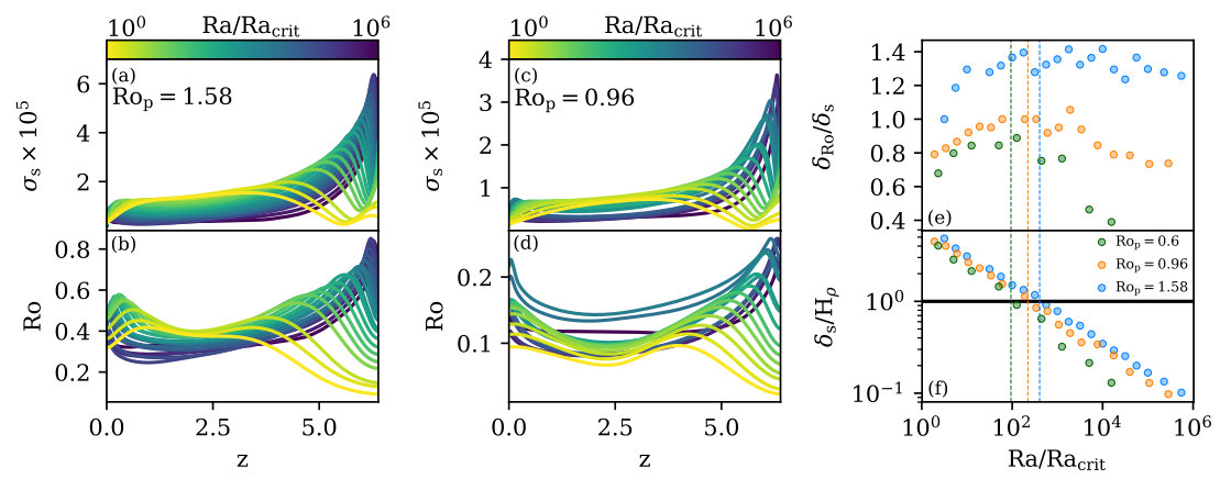 Figure 1
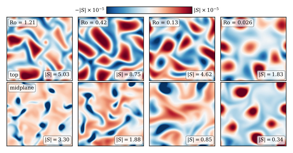 Figure 2
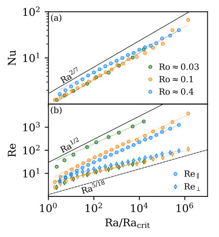 Figure 3
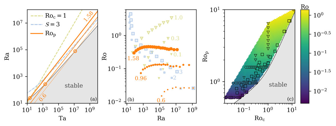 Figure 4
| (Ra, Ta) | (Ra, Ta) | |
|---|---|---|
| 0.60 | () | () |
| 0.96 | () | () |
| 1.58 | () | () |
| Ra | Ta | Ro | Ra | Ta | Ro | (nz, nx, ny) | Ro | Re∥ | Re⟂ | Nu | |||
|---|---|---|---|---|---|---|---|---|---|---|---|---|---|
| Constant , path III | |||||||||||||
| 1.8 | 4.1 | 0.60 | 1.4 | 3.0 | 1.03 | 0.067 | 1.1 | 0.51 | (256, 32, 32) | 0.015 | 19.4 | 2.5 | 1.2 |
| 1.2 | 5.2 | 0.60 | 9.2 | 3.8 | 1.03 | 0.015 | 3.0 | 0.07 | (2048, 64, 64) | 0.026 | 1771 | 32.0 | 15.4 |
| 5.2 | 4.6 | 0.96 | 3.8 | 3.4 | 1.64 | 0.333 | 1.13 | 2.28 | (64, 64, 64) | 0.074 | 4.2 | 2.5 | 1.2 |
| 3.8 | 3.1 | 0.96 | 2.8 | 2.3 | 1.64 | 0.035 | 6.0 | 0.12 | (2048, 64, 64) | 0.129 | 3906 | 113 | 66.9 |
| 7.9 | 1.0 | 1.58 | 5.8 | 7.4 | 2.70 | 0.888 | 1.56 | 4.44 | (64, 64, 64) | 0.303 | 4.4 | 4.9 | 1.7 |
| 1.4 | 9.7 | 1.58 | 1.0 | 7.2 | 2.70 | 0.119 | 10.0 | 0.30 | (512, 128, 128) | 0.376 | 1257 | 94.9 | 40.1 |
| Constant , path II | |||||||||||||
| 8.6 | 8.6 | 0.74 | 6.3 | 6.3 | 1.26 | 0.1 | 1.47 | 0.68 | (128, 128, 128) | 0.051 | 40.2 | 6.7 | 2.2 |
| 2.6 | 2.6 | 1.13 | 1.9 | 1.9 | 1.93 | 0.1 | 4.64 | 0.39 | (256, 512, 512) | 0.27 | 565 | 53.2 | 33.3 |
| 1.4 | 1.6 | 1.01 | 1.1 | 1.2 | 1.72 | 0.3 | 1.47 | 1.90 | (64, 128, 128) | 0.124 | 11.3 | 5.4 | 1.8 |
| 1.1 | 1.2 | 2.29 | 7.8 | 8.6 | 3.93 | 0.3 | 14.7 | 0.65 | (192, 384, 384) | 0.808 | 529 | 83.5 | 27.3 |
| 5.5 | 5.5 | 1.65 | 4.0 | 4.0 | 2.82 | 1.0 | 1.47 | 4.84 | (64, 128, 128) | 0.303 | 3.6 | 4.4 | 1.5 |
| 2.8 | 2.8 | 6.39 | 2.0 | 2.0 | 10.93 | 1.0 | 100 | 0.82 | (256, 512, 512) | 3.357 | 1099 | 220 | 46.6 |
| Constant , path I | |||||||||||||
| 1.9 | 1.1 | 10.00 | 1.4 | 7.9 | 17.12 | 13.2 | 2.0 | 9.91 | (64, 64, 64) | 3.668 | 3.0 | 10.2 | 1.7 |
| 3.0 | 1.1 | 0.70 | 2.2 | 8.1 | 1.20 | 0.052 | 2.0 | 0.30 | (512, 128, 128) | 0.053 | 242 | 17.9 | 6.0 |
| 3.0 | 2.0 | 10.00 | 2.2 | 1.5 | 17.12 | 12.2 | 3.0 | 9.48 | (64, 64, 64) | 4.418 | 5.0 | 15.5 | 2.1 |
| 1.3 | 5.6 | 0.80 | 9.7 | 4.2 | 1.37 | 0.048 | 3.0 | 0.23 | (512, 128, 128) | 0.08 | 592 | 33.4 | 13.6 |
Peer Reviews
No public reviews on file for this paper yet. If you reviewed it on a platform where reviews are public (OpenReview, ICLR, NeurIPS, ICML), you can paste yours below so the community can read it here.
Videos
No videos yet. Explain this paper in a talk, walkthrough, or lecture? Add one.
Predicting the Rossby number in convective experiments
Dept. Astrophysical & Planetary Sciences, University of Colorado – Boulder, Boulder, CO 80309, USA
Laboratory for Atmospheric and Space Physics, Boulder, CO 80303, USA
Cathryn M. Manduca
Laboratory for Atmospheric and Space Physics, Boulder, CO 80303, USA
Dept. Astrophysical & Planetary Sciences, University of Colorado – Boulder, Boulder, CO 80309, USA
Laboratory for Atmospheric and Space Physics, Boulder, CO 80303, USA
Department of Physics and Astronomy, Bates College, Lewiston, ME 04240, USA
Geoffrey M. Vasil
University of Sydney School of Mathematics and Statistics, Sydney, NSW 2006, Australia
(Received October 19, 2018; Revised January 14, 2019; Accepted January 15, 2019)
Abstract
The Rossby number is a crucial parameter describing the degree of rotational constraint on the convective dynamics in stars and planets. However, it is not an input to computational models of convection but must be measured ex post facto. Here, we report the discovery of a new quantity, the Predictive Rossby number, which is both tightly correlated with the Rossby number and specified in terms of common inputs to numerical models. The Predictive Rossby number can be specified independent of Rayleigh number, allowing suites of numerical solutions to separate the degree of rotational constraint from the strength of the driving of convection. We examine the scaling of convective transport in terms of the Nusselt number and the degree of turbulence in terms of the Reynolds number of the flow, and we find scaling laws nearly identical to those in nonrotational convection at low Rossby number when the Predictive Rossby number is held constant. Finally, we describe the boundary layers as a function of increasing turbulence at constant Rossby number.
convection — hydrodynamics — turbulence — dynamo — Sun: rotation
††journal: ApJ
1 Introduction
Rotation influences the dynamics of convective flows in stellar and planetary atmospheres. Many studies on the fundamental nature of rotating convection in both laboratory and numerical settings have provided great insight into the properties of convection in both the rapidly rotating regime and the transition to the rotationally unconstrained regime (King et al., 2009; Zhong et al., 2009; Schmitz & Tilgner, 2009; King et al., 2012; Julien et al., 2012; King et al., 2013; Ecke & Niemela, 2014; Stellmach et al., 2014; Cheng et al., 2015; Gastine et al., 2016) The scaling behavior of heat transport, the nature of convective flow structures, and the importance of boundary layer-bulk interactions in driving dynamics are well known. Yet, we do not know of any simple procedure for predicting the magnitude of vortical flow gradients purely from experimental control parameters, such as bulk rotation rate and thermal input.
In the astrophysical context, many studies of rotating convection have investigated questions inspired by the solar dynamo (Glatzmaier & Gilman, 1982; Busse, 2002; Brown et al., 2008, 2010, 2011; Augustson et al., 2012; Guerrero et al., 2013; Käpylä et al., 2014). Even when these simulations nominally rotate at the solar rate, they frequently produce distinctly different behaviors than the true Sun, such as anti-solar differential rotation profiles (Gastine et al., 2014; Brun et al., 2017). It seems that these differences occur because the simulations produce less rotationally constrained states than the Sun. The influence of rotation results from the local shear gradients, and these are not direct input parameters. Recent simulations predict significant rotational influence in the deep solar interior, which can drastically affect flows throughout the solar convection zone (Featherstone & Hindman, 2016; Greer et al., 2016). In the planetary context, the balance between magnetic and rotational forces likely leads to the observed differences between ice giant and gas giant dynamos in our solar system (Soderlund et al., 2015). The work of Aurnou & King (2017) demonstrates the importance of studying a dynamical regime with the proper balance between Lorentz, Coriolis, and inertial forces when modeling astrophysical objects such as planetary dynamos.
In short, simulations must achieve the proper rotational balance if they are to explain the behavior of astrophysical objects. In Boussinesq studies, rotational constraint is often measured by comparing dynamical and thermal boundary layers or deviation in heat transport from the non-rotating state (King et al., 2012; Julien et al., 2012; King et al., 2013). Such measurements are not available for astrophysical objects, where the degree of rotational influence is best assessed by the ratio between nonlinear advection magnitude and the linear Coriolis accelerations. The Rossby number is the standard measure of this ratio,
[TABLE]
where denotes the bulk rotation vector. Many proxies for the dynamical Rossby number exist that are based solely on input parameters, most notably the convective Rossby number. However, all proxies produce imperfect predictions for the true dynamically relevant quantity.
In this letter, we demonstrate an emperical method of predicting the output Rossby number of convection in a simple stratified system.
In Anders & Brown (2017) (hereafter AB17), we studied non-rotating compressible convection without magnetic fields in polytropic atmospheres. In this work, we extend AB17 to rotationally-influenced, -plane atmospheres (e.g., Brummell et al., 1996, 1998; Calkins et al., 2015). We determine how the input parameters we studied previously, which controlled the Mach and Reynolds numbers of the evolved flows, couple with the Taylor number (Ta, Julien et al., 1996), which sets the magnitude of the rotational vector.
In section 2, we describe our experiment and paths through parameter space. In section 3, we present the results of our experiments and in section 4 we offer concluding remarks.
2 Experiment
We study fully compressible, stratified convection under precisely the same atmospheric model as in AB17, but here we have included rotation. We study polytropic atmospheres with density scale heights and a superadiabatic excess of such that flows are at low Mach number. We study a domain in which the gravity, , and rotational vector, , are antiparallel (as in e.g., Julien et al., 1996; Brummell et al., 1996).
We evolve the velocity (), temperature (), and log density () according to the Fully Compressible Navier-Stokes equations in the same form presented in AB17, with the addition of the Coriolis term, , to the left-hand side of the momentum equation. We impose impenetrable, stress-free, fixed-temperature boundary conditions at the top and bottom of the domain.
We specify the kinematic viscosity (), thermal diffusivity (), and strength of rotation () at the top of the domain by choosing the Rayleigh number (Ra), Prandtl number (Pr), and Taylor number (Ta),
[TABLE]
where is the depth of the domain as defined in AB17, is the specific entropy difference between the top and bottom of the atmosphere, and the specific heat at constant pressure is with . Throughout this work we set Pr = 1. The Taylor number relates to the often-quoted Ekman number by the equality .
Due to stratification, Ra and Ta both grow with depth as (Ra,Ta) (see AB17). We nondimensionalize our atmospheres at the top of the domain, and so all values of Ra and Ta quoted in this work are the minimal value of Ra and Ta in the domain at . For direct comparison to Boussinesq studies, past work has found that the value of Ra at the atmospheric midplane () varies minimally with increasing stratification (Unno et al., 1960). For the atmospheres presented in this work, midplane Ra and Ta values are larger than reported top-of-atmosphere values by a factor of 70, and values at the bottom of the atmosphere are larger by 400.
When Ta is large, the wavenumber of convective onset increases according to (Chandrasekhar, 1961; Calkins et al., 2015). We study horizontally-periodic, 3D Cartesian domains with extents of and . At large values of Ta, these domains are tall and skinny, as in Stellmach et al. (2014). We evolve our simulations using the Dedalus111http://dedalus-project.org/ pseudospectral framework, and our numerical methods are identical to those presented in AB17. The supplemental materials of this paper include a .tar file which contains the code used to perform the simulations in this work, and this tarball is also published online in a Zenodo repository (Anders et al., 2019).
The critical value of Ra at which rapidly rotating convection onsets also depends on Ta (see the black line in figure 1a), roughly according to (Chandrasekhar, 1961; Calkins et al., 2015). Even taking account of linear theory, the dependence of the evolved nonlinear fluid flows on the input parameters makes predicting the rotational constraint very challenging. We will explore three paths through Ra-Ta space:
[TABLE]
Paths on constraint I are at constant supercriticality, (blue dash-dot line in figure 1a). Paths on constraint II (green dashed line in figure 1a) are at a constant value of the classic convective Rossby number,
[TABLE]
which has provided (e.g., Julien et al., 1996; Brummell et al., 1996) a common proxy for the degree of rotational constraint. This parameter measures the importance of buoyancy relative to rotation without involving dissipation. Paths on constraint III (e.g., orange solid lines in figure 1a) set constant a ratio which we call the “Predictive Rossby number,”
[TABLE]
Unlike paths through parameter space which hold constant, paths with constant feel changes in diffusivities but not the depth of the domain. To our knowledge, these paths have not been reported in the literature, although the importance of has been independently found by King et al. (2012) using a boundary layer analysis. We compare our results to their theory in Section 4.
In this work, we primarily study three values of . These values are shown in Fig. 1a and Table 1. Table 1 lists the values of (Ra, Ta) for each value of , and also the maximum value of (Ra, Ta) studied in this work for each path. We additionally walked two pathways at constant supercriticality (constraint I, ) and three pathways at constant convective Rossby number (constraint II, ). Full details on all cases are provided in Appendix A and the supplemental materials.
3 Results
In our stratified domains, for , a best-fit to results from a linear stability analysis provides and for direct onset of convection. In figure 1a, the value of Ra is shown. Sample paths for each criterion in equation 3 through this parameter space are also shown. In this work, we often find it instructive to use one critical Ra for an entire path. This is determined by the intersection of the onset curve and path (indicated by the orange circles in figure 1a, and quoted in Table 1). In the high Ta regime, we find that .
In figure 1b, we display the evolution of Ro with increasing Ra along various paths through parameter space. We find that Ro increases on constant paths, decreases on constant paths, and remains roughly constant along constant paths. In figure 1c, the value of Ro is shown simultaneously as a function of and for all experiments conducted in this study. We find a general power-law of the form . In the rotationally-dominated regime where and (see Eqn. 6), we find , and Ro can be said to be a function of alone. Under this assumption, we report a scaling of . In the less rotationally dominated regime of and , we find .
In figure 2, sample snapshots of the evolved entropy field in the - plane near the top and at the middle of the domain are shown. In the left column, flows are at and resemble the classic granular structure of nonrotating convection (see e.g., figure 2 in AB17), where strong narrow downflow lanes punctuate broad upwellings. The narrow downflows at the top organize themselves into intense coherent structures at the midplane, and at the midplane the downflows have much stronger entropy fluctuations than the broad and slower upflows.
Ro decreases from left to right into the rotationally constrained regime. As Ro decreases, the narrow downflow lanes begin to disappear and the flows at midplane become more symmetric. In the rotationally constrained regime (), the convective structures are distinctly different. Here we observe dynamically persistent, warm upflow columns surrounded by bulk weak downflow regions. At the midplane, the upflow columns have substantially higher entropy perturbations than the surrounding weak downflows which sheathe them, and the locations of the columns are tightly correlated with their positions at the top of the domain. These quasi-two-dimensional dynamics are similar to those seen in rapidly rotating Rayleigh-Bénard convection (e.g., Stellmach et al., 2014). The select cases displayed in figure 2 each have an evolved volume-averaged (defined below in equation 6).
We measure the Nusselt number (Nu), which quantifies heat transport in a convective solution, as defined in AB17. In figure 3a, we plot Nu as a function of at fixed . We find that for . In the regime of , these scaling laws are indistinguishable from a classic Ra2/7 power law scaling, which is observed in nonrotating Rayleigh-Bénard and stratified convection (Ahlers et al., 2009, AB17). Our results seem consistent with the stress-free, rotating Rayleigh-Bénard convection results of Schmitz & Tilgner (2009), whose re-arranged Eqn. 7 returns a best-fit of at fixed . Their work primarily spans the transition regime between rotationally constrained and unconstrained convection, and so it is perhaps not surprising that their power law is a blend of our rotationally-constrained power law and the fairly rotationally unconstrained at .
Flows are distinctly different parallel to and perpendicular from the rotation vector, which aligns with gravity and stratification. We measure two forms of the RMS Reynolds number,
[TABLE]
where the length scale in is the wavelength of convective onset, and is related to the horizontal extent of our domain (see section 2). From our work in AB17, we expect the RMS velocity to scale as . By definition, , and is a constant set by the stratification while . Along paths of constant , we thus expect and when Pr is held constant.
In figure 3b, we plot and as a function of Ra at fixed . We find that and for . These scalings are similar to but slightly weaker than our predictions in all cases. However, the scaling of , is once again a power law observed frequently in nonrotating convection (Ahlers et al., 2009, AB17). We also observe that collapses for each track, while experiences an offset to larger values as shrinks. The offset in is unsurprising, because more rotationally constrained flows result in smaller boundary layers relative to the vertical extent of our stratified domain. The horizontal extent of our domain scales with the strength of rotation, and so regardless of , flows perpendicular to the rotational and buoyant direction are comparably turbulent at the same . We find and are, respectively, good proxies for the horizontal and perpendicular resolution required to resolve an experiment.
Figure 4 shows time- and horizontally-averaged profiles of Ro and the standard deviation of the entropy, . Figures 4a&b show these profiles for (), while Figures 4c&d show these profiles for (). The transition in profile behavior from low Ra (yellow) to high Ra (purple) is denoted by the color of the profile. As Ra increases at a constant value of , both the thermal () and dynamical (Ro) boundary layers become thinner. We measure the thickness of the thermal boundary layer () at the top of the domain by finding the location of the first maxima of away from the boundary. We measure the thickness of the Ro boundary layer () in the same manner. In figure 4e, we plot , the ratio of the sizes of these two boundary layers. As anticipated, the dynamical boundary layer () becomes relatively thinner with respect to the thermal boundary layer () as Ro and decrease. However, the precise scaling of this boundary layer ratio with and Ra is unclear, and we cannot immediately compare these ratios to similar measures from the Rayleigh-Bénard convection literature, such as Fig. 5 of King et al. (2013). They measure the dynamical boundary layer thickness as the peak location of the horizontal velocities, but our horizontal velocities are subject to stress-free boundary conditions, and we find that the maxima of horizontal velocities occur precisely at the boundaries. In figure 4f, we plot in units of the density scale height at the top of the atmosphere, and we plot vertical lines when this crosses 1. We find no systematic change in behavior when is smaller than the local density scale height.
4 Discussion
In this letter, we studied low-Mach-number, stratified, compressible convection under the influence of rotation. We examined three paths through Ra-Ta space, and showed that the newly-defined Predictive Rossby number, , determines the value of the evolved Rossby number.
Shockingly, along these constant pathways, particularly when , we find and . These scalings are indistinguishable from the scalings of Re and Nu with Ra in non-rotating Boussinesq convection (Ahlers et al., 2009). Julien et al. (2012) theorized that in the rapidly rotating asymptotic limit, . Thus, at fixed Ta, a very sharp scaling law is expected. At a fixed Ta = , Stellmach et al. (2014) found that the Ra3/2 scaling described the results of stress-free DNS in Boussinesq cylinders very well. Gastine et al. (2016) studied Boussinesq convection in spherical shells with no-slip boundaries, and also found good agreement with the theory of Julien et al. (2012) for various Ra at .
Here, when we run simulations at fixed , the value of Ta is coupled to the value of Ra, and both increase simultaneously. Recasting the scaling of Julien et al. (2012) into this perspective, we find , where in this final result we use the value of the whole path, such as those specified in Table 1. This scaling is much weaker than the law we find here. We leave it to future work to explain this discrepancy between Boussinesq theory and our observed Nu vs. Ra scaling.
In this work, we experimentally arrived at the scaling in , but this relationship was independently discovered by King et al. (2012). Arguing that the thermal boundary layers should scale as and rotational Ekman boundary layers should scale as , they expect these boundary layers to be equal in size when . They demonstrate that when flows are in the transitional regime, and for , flows are rotationally constrained. We remind the reader that Boussinesq values of Ra and Ta are not the same as their values in our stratified domains here, as diffusivities change with depth (see section 2). Taking into account this change with depth, our simulations fall in King et al. (2012)’s rotationally constrained () and near-constrained transitional regime (). The measured values of Ro in Fig. 1b and the observed dynamics in Fig. 2 agree with this interpretation.
We note briefly that the scaling is very similar to another theorized boundary between fully rotationally constrained convection and partially constrained convection predicted in Boussinesq theory, of (Julien et al., 2012; Gastine et al., 2016). This Ta4/5 scaling also arises through arguments of geostrophic balance in the boundary layers, and is a steeper scaling than the Ta3/4 scaling present in . This suggests that at sufficiently low , a suite of simulations across many orders of magnitude of Ra will not only have the same volume-averaged value of Ro (as in Fig. 1b), but will also maintain proper force balances within the boundary layers.
Our results suggest that by choosing the desired value of , experimenters can select the degree of rotational constraint present in their simulations. We find that , which is within 2 of the estimate in King et al. (2013), who although defining Ro very differently from our vorticity-based definition here, find . We note briefly that they claim that the value of Ro is strongly dependent upon the Prandtl number studied, and that low Ro can be achieved at high Pr without achieving a rotationally constrained flow. We studied only here, and leave it to future work to determine if the scaling of is the correct scaling to predict the evolved Rossby number.
Despite the added complexity of stratification and despite our using stress-free rather than no-slip boundaries, the boundary layer scaling arguments put forth in King et al. (2012) seem to hold up in our systems. This is reminiscent of what we found in AB17, in which convection in stratified domains, regardless of Mach number, produced boundary-layer dominated scaling laws of Nu that were nearly identical to the scaling laws found in Boussinesq Rayleigh-Bénard convection.
We close by noting that once is chosen such that a convective system has the same Rossby number as an astrophysical object of choice, it is straightforward to increase the turbulent nature of simulations by increasing Ra, just as in the non-rotating case. Although all the results reported here are for a Cartesian geometry with antiparallel gravity and rotation, preliminary 3D spherical simulations suggest that also specifies Ro in more complex geometries (Brown et al. 2019 in prep).
We thank Jon Aurnou and the anonymous referee who independently directed us to the work of King et al. (2012) during the review process, which greatly helped us understand the results of the experiments here. We further thank the anonymous referee for other helpful and clarifying suggestions. This work was supported by NASA Headquarters under the NASA Earth and Space Science Fellowship Program – Grant 80NSSC18K1199. EHA further acknowledges the University of Colorado’s George Ellery Hale Graduate Student Fellowship. This work was additionally supported by NASA LWS grant number NNX16AC92G. Computations were conducted with support by the NASA High End Computing (HEC) Program through the NASA Advanced Supercomputing (NAS) Division at Ames Research Center on Pleiades with allocation GID s1647.
Appendix A Table of Simulations
Information for select simulations in this work are shown in Table 2. The simulation at minimum (Ra, Ta) and maximum (Ra, Ta) for each of the , , and paths in Fig. 1b are shown. This information for the displayed simulations and all other simulations in this work is included as a .csv file in the supplemental materials and is published online in a Zenodo repository (Anders et al., 2019).
The reference list from the paper itself. Each links out to its DOI / PubMed record.
- 1Ahlers et al. (2009) Ahlers, G., Grossmann, S., & Lohse, D. 2009, Rev. Mod. Phys., 81, 503
- 2Anders & Brown (2017) Anders, E. H., & Brown, B. P. 2017, Physical Review Fluids, 2, 083501
- 3Anders et al. (2019) Anders, E. H., Manduca, C. M., Brown, B. P., Oishi, J. S., & Vasil, G. M. 2019, Supplemental Materials: Predicting the Rossby number in convective experiments, v.1.0, Zenodo, doi:10.5281/zenodo.2539500
- 4Augustson et al. (2012) Augustson, K. C., Brown, B. P., Brun, A. S., Miesch, M. S., & Toomre, J. 2012, Ap J, 756, 169
- 5Aurnou & King (2017) Aurnou, J. M., & King, E. M. 2017, Proceedings of the Royal Society of London Series A, 473, 20160731
- 6Brown et al. (2008) Brown, B. P., Browning, M. K., Brun, A. S., Miesch, M. S., & Toomre, J. 2008, Ap J, 689, 1354
- 7Brown et al. (2010) —. 2010, Ap J, 711, 424
- 8Brown et al. (2011) Brown, B. P., Miesch, M. S., Browning, M. K., Brun, A. S., & Toomre, J. 2011, Ap J, 731, 69