R3-DLA (Reduce, Reuse, Recycle): A More Efficient Approach to Decoupled Look-Ahead Architectures
Sushant Kondguli, Michael Huang

TL;DR
This paper introduces R3-DLA, an optimized decoupled look-ahead architecture that significantly improves single-thread performance by making look-ahead agents more efficient, achieving an average speedup of 1.4 over existing microarchitectures.
Contribution
It proposes a set of optimizations for decoupled look-ahead architectures, enhancing efficiency and utility, leading to notable performance improvements.
Findings
Achieves an average speedup of 1.4 over state-of-the-art microarchitecture.
Enhances single-thread performance across diverse benchmarks.
Demonstrates broad applicability of optimized DLA in general-purpose computing.
Abstract
Modern societies have developed insatiable demands for more computation capabilities. Exploiting implicit parallelism to provide automatic performance improvement remains a central goal in engineering future general-purpose computing systems. One approach is to use a separate thread context to perform continuous look-ahead to improve the data and instruction supply to the main pipeline. Such a decoupled look-ahead (DLA) architecture can be quite effective in accelerating a broad range of applications in a relatively straightforward implementation. It also has broad design flexibility as the look-ahead agent need not be concerned with correctness constraints. In this paper, we explore a number of optimizations that make the look-ahead agent more efficient and yet extract more utility from it. With these optimizations, a DLA architecture can achieve an average speedup of 1.4 over a…
Click any figure to enlarge with its caption.
 Figure 1
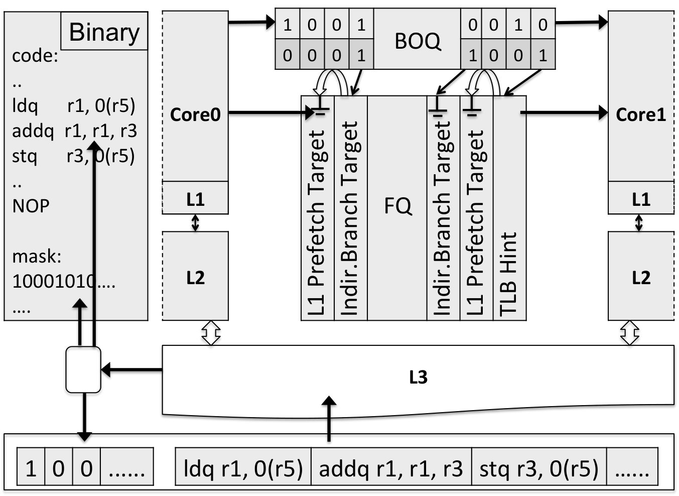 Figure 2
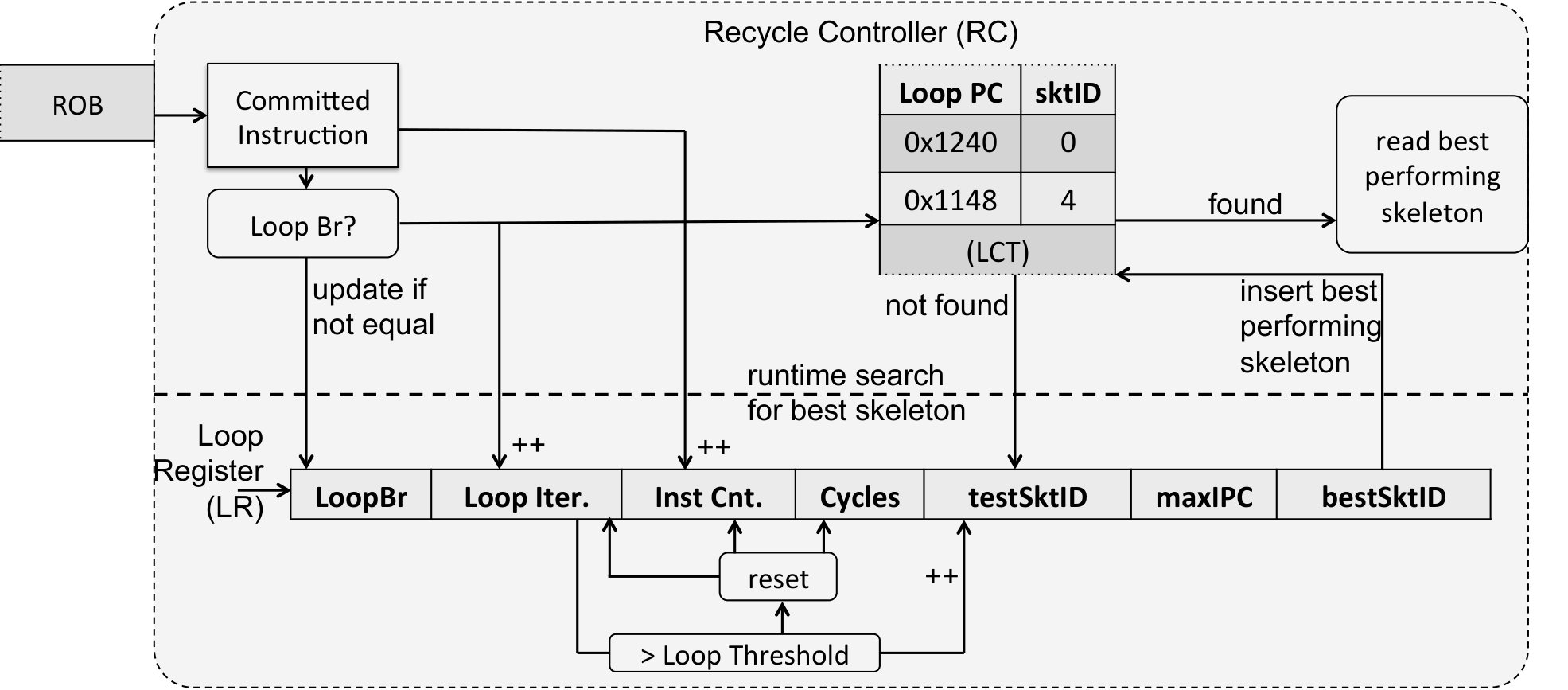 Figure 3
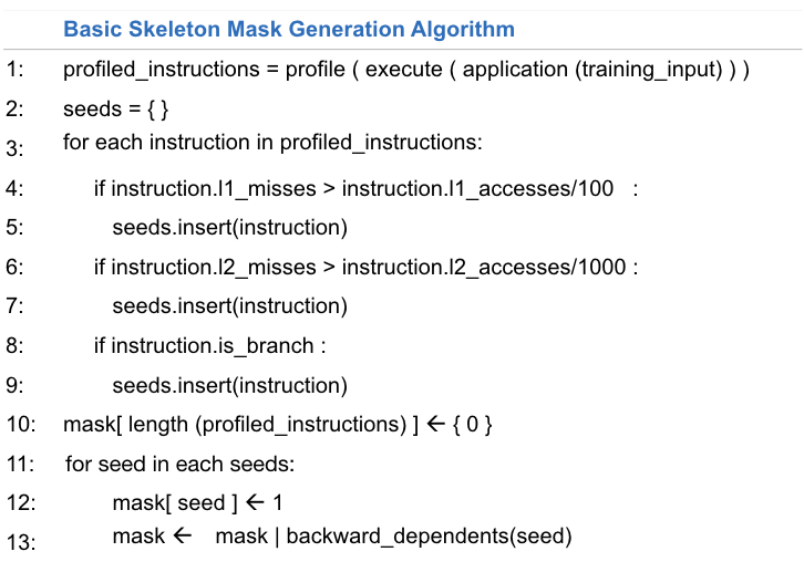 Figure 4
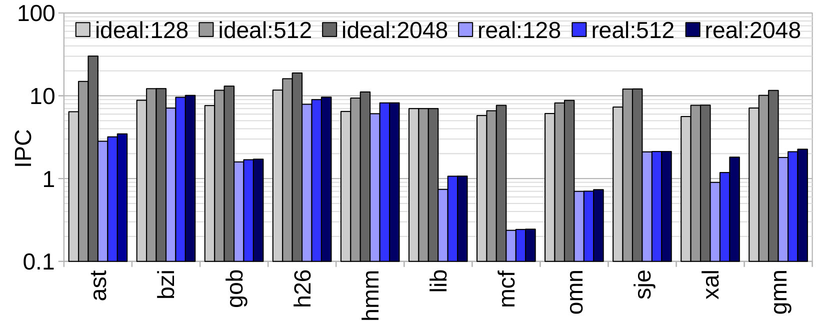 Figure 5
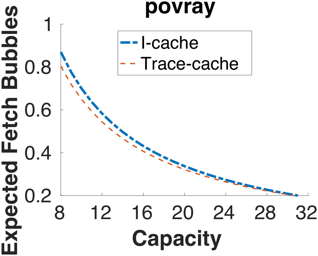 Figure 6
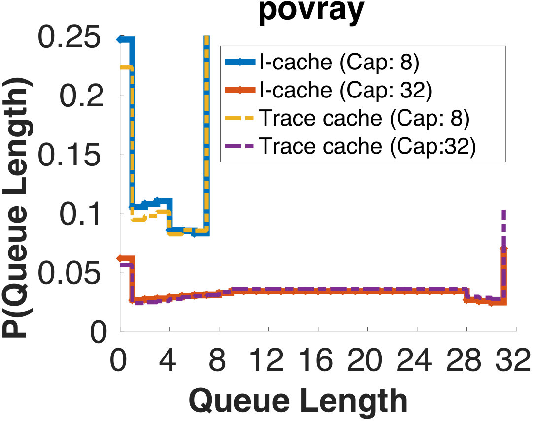 Figure 7
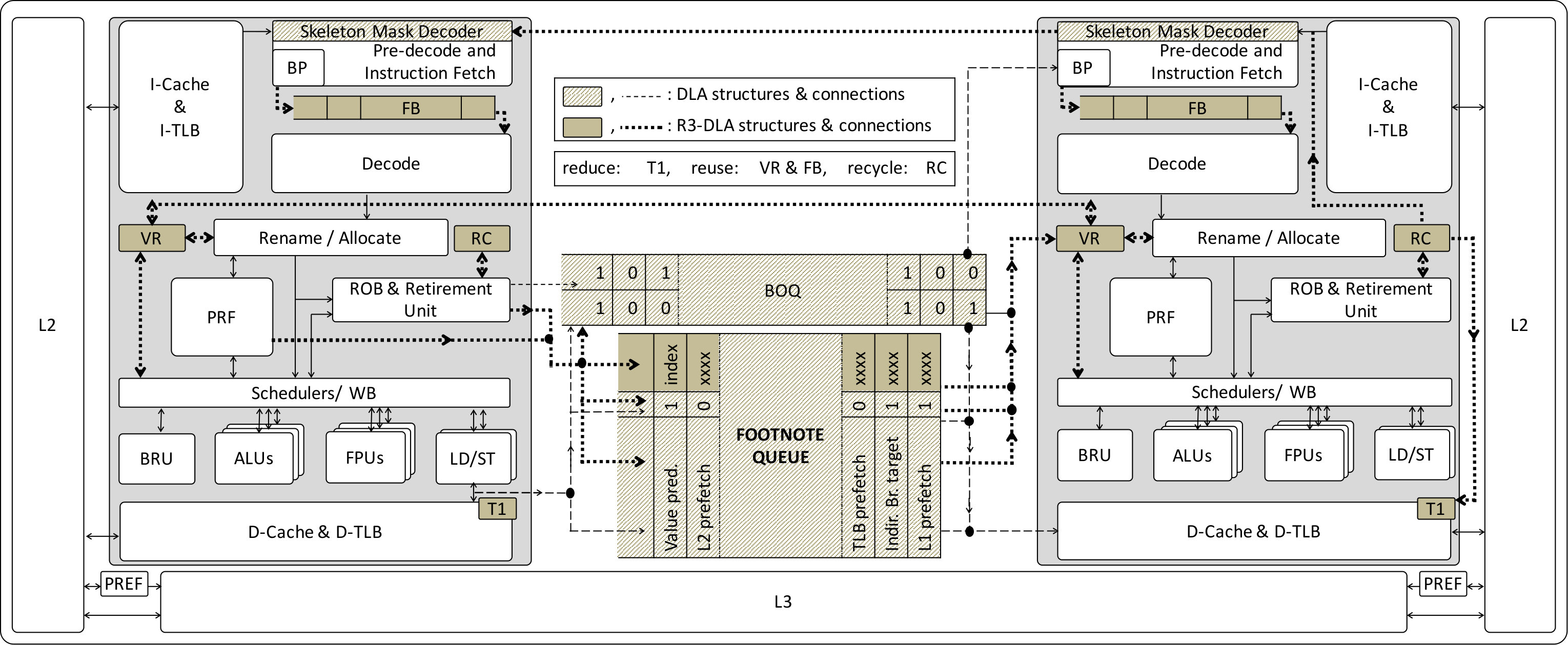 Figure 8
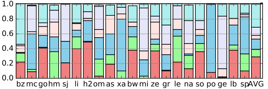 Figure 9
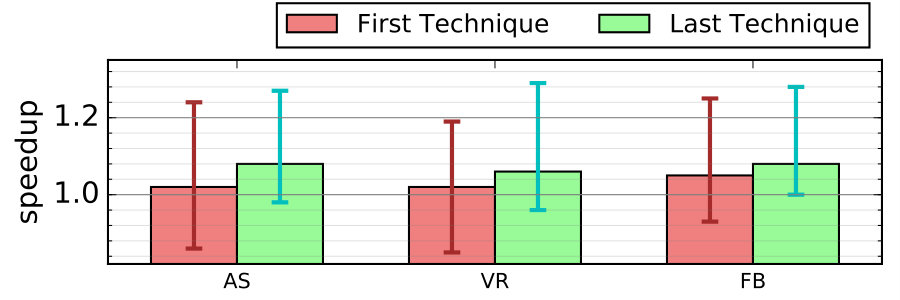 Figure 10
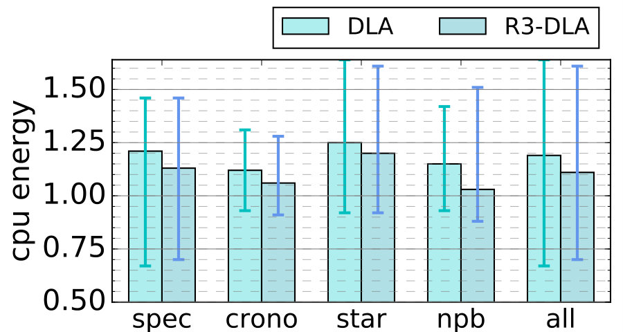 Figure 11
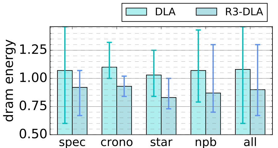 Figure 12
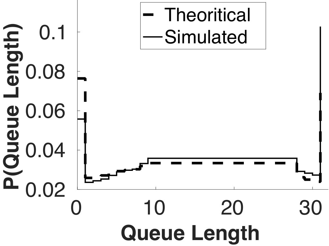 Figure 13
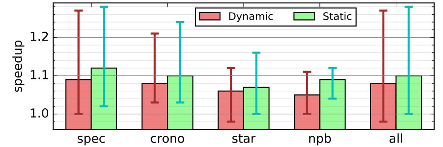 Figure 14
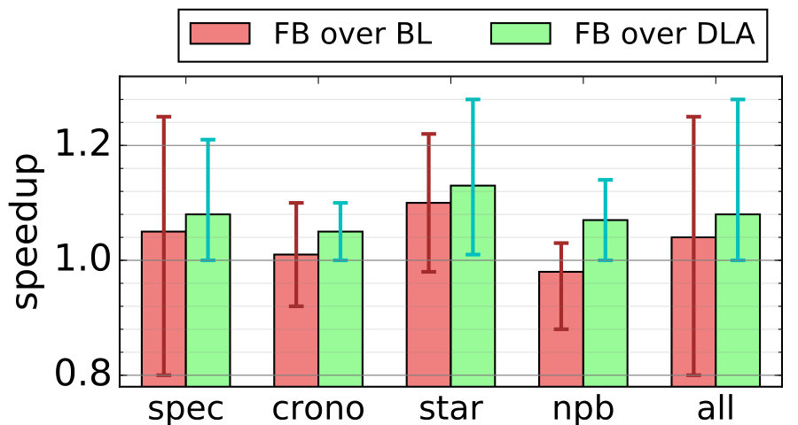 Figure 15
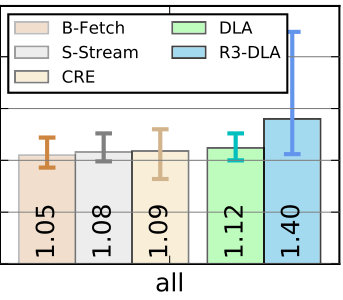 Figure 16
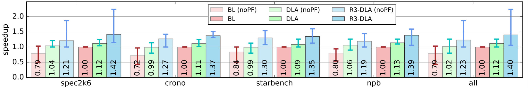 Figure 17
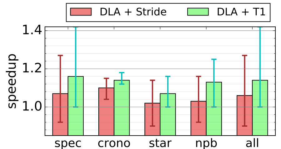 Figure 18
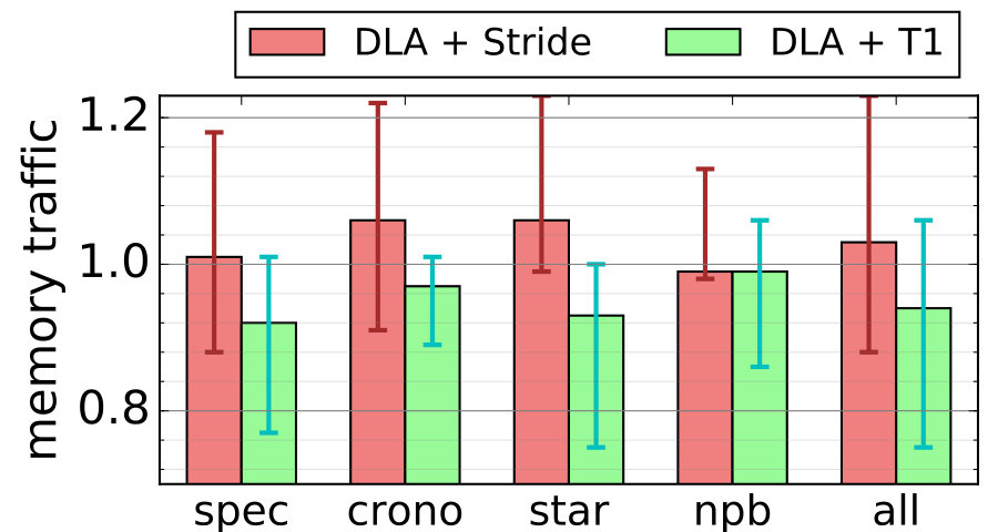 Figure 19
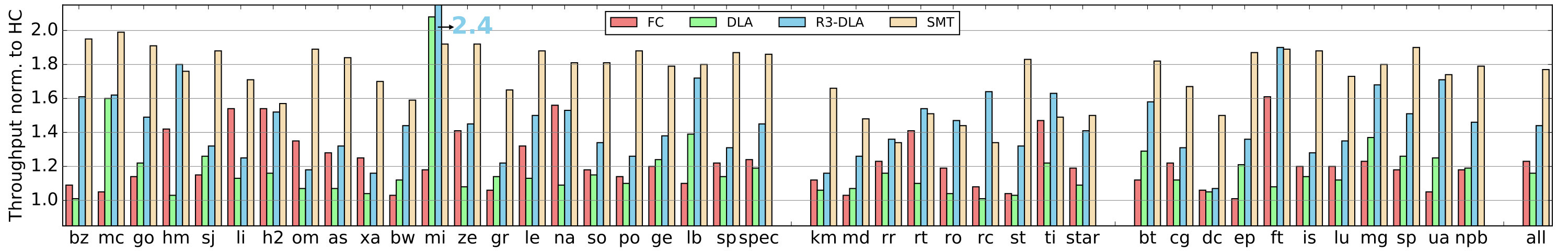 Figure 20
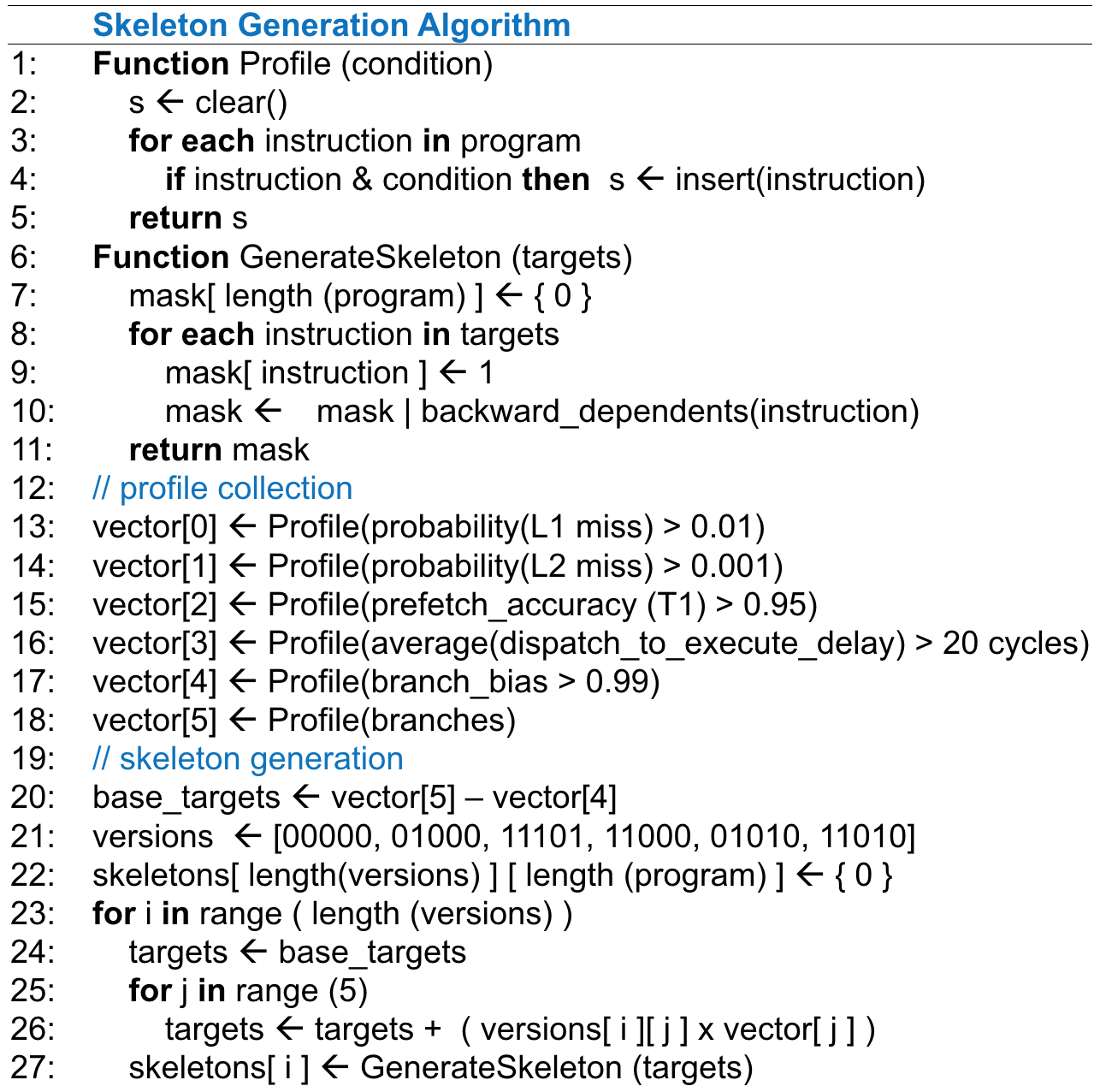 Figure 21
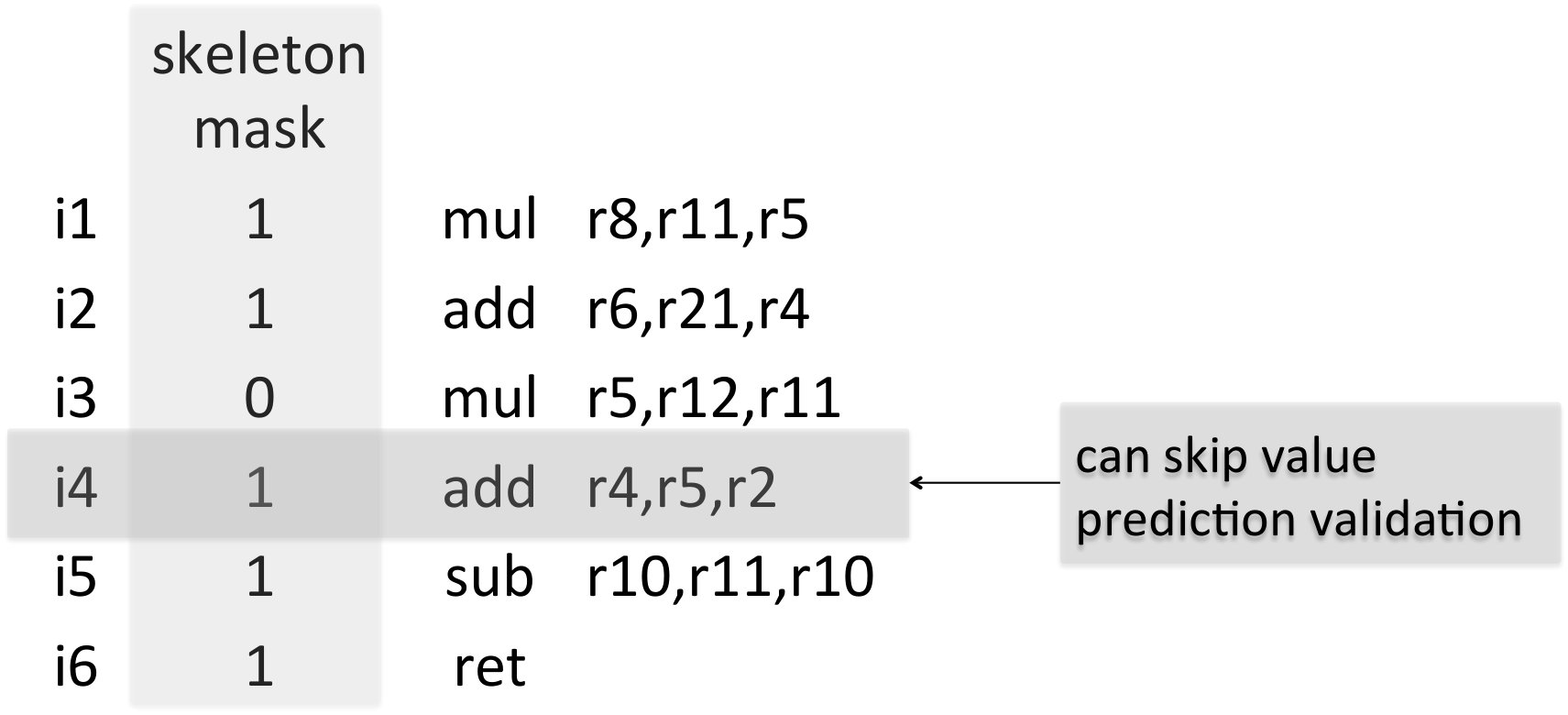 Figure 22
| Processing Node | 20-stage pipeline, out-of-order, 4-wide, 192 ROB, 96 LSQ, 128INT/128FP PRF, 4INT/ 2MEM/ 4FP FUs, Tage SC-L Predictor (configured as the 256kBits predictor described in [92]), 4K Entry BTB, 32-entry RAS |
| Operating Points | 0.8V, 3.0GHz |
| L1 Caches | 32KB I-cache and 32KB D-cache, 4-way, 64B blocks, 3 ports, 1ns, 32 MSHRs, LRU |
| L2 Cache | 256KB, 8-way, 64B blocks, 2 ports, 3ns, 32 MSHRs, LRU, BOP [71] |
| L3 Cache | 2MB, 16-way, 64B blocks, 12ns, LRU |
| Main Memory | 4GB, DDR3 1600MHz, 1.5V, 2 channels, 2 ranks/channel, 8 banks/rank, tRCD=13.75ns, tRAS=35ns, tFAW=30ns, tWTR=7.5ns, tRP=13.75ns |
| DLA Support | |
| BOQ | 512 entries (512x2 bits = 128B) |
| FQ | 128 entries (128x64 bits = 1KB) |
| R3-DLA Support | |
| T1 | 16 prefetching entries (512B) |
| FB | 32 instructions (256B) |
| VPT | 32 Entries (32x64 bits = 256B) (used by VR) |
| LCT | 16 Entries (136B) (used by RC) |
| D | X | C | Dyn. Energy | Dyn. Power | Static Power | Power | ||
|---|---|---|---|---|---|---|---|---|
| DLA | LT | 49% | 48% | 48% | 48% | 54% | 94% | 71% |
| MT | 77% | 86% | 100% | 88% | 96% | 99% | 97% | |
| R3-DLA | LT | 35% | 29% | 29% | 30% | 42% | 93% | 64% |
| MT | 77% | 82% | 100% | 80% | 110% | 95% | 103% |
| strided | others | |||||||
|---|---|---|---|---|---|---|---|---|
| config. | BL | BL + stride | DLA | DLA + T1 | BL | BL + stride | DLA | DLA + T1 |
| mean | 12.4 | 8.4 | 5.9 | 2.1 | 7.4 | 6.9 | 6.1 | 4.8 |
| median | 10.0 | 4.8 | 4.0 | 1.1 | 3.9 | 3.5 | 2.8 | 3.2 |
Peer Reviews
No public reviews on file for this paper yet. If you reviewed it on a platform where reviews are public (OpenReview, ICLR, NeurIPS, ICML), you can paste yours below so the community can read it here.
Videos
No videos yet. Explain this paper in a talk, walkthrough, or lecture? Add one.
Taxonomy
TopicsParallel Computing and Optimization Techniques · Advanced Data Storage Technologies · Cloud Computing and Resource Management
R3-DLA (Reduce, Reuse, Recycle): A More Efficient Approach to Decoupled
Look-Ahead Architectures
Sushant Kondguli and Michael Huang Department of Electrical and Computer Engineering
University of Rochester, Rochester, NY
{sushant.kondguli, michael.huang}@rochester.edu
Abstract
Modern societies have developed insatiable demands for more computation capabilities. Exploiting implicit parallelism to provide automatic performance improvement remains a central goal in engineering future general-purpose computing systems. One approach is to use a separate thread context to perform continuous look-ahead to improve the data and instruction supply to the main pipeline. Such a decoupled look-ahead (DLA) architecture can be quite effective in accelerating a broad range of applications in a relatively straightforward implementation. It also has broad design flexibility as the look-ahead agent need not be concerned with correctness constraints. In this paper, we explore a number of optimizations that make the look-ahead agent more efficient and yet extract more utility from it. With these optimizations, a DLA architecture can achieve an average speedup of 1.4 over a state-of-the-art microarchitecture for a broad set of benchmark suites, making it a powerful tool to enhance single-thread performance.
Index Terms:
single thread performance; decoupled lookahead architecture;
I Introduction
Modern societies have developed insatiable demands for more computation capabilities. While in certain segments, delivering higher performance via intense human labor (manual parallelization and performance tuning) is justifiable, in many other situations, such effort is not necessarily effective nor is it particularly efficient when the extra resources (energy and loss of productivity) are properly accounted for. Automatic performance improvement remains a central goal in engineering future general-purpose computing systems [44]. After all, the systems have always been designed to increase automation and productivity and to free human from drudgery (including debugging a parallel code).
The two traditional drivers for single-thread performance (faster cycles and advancements in microarchitecture) have all but stopped in recent years – and for good reasons, since further gains from these approaches will come at significant costs. However, the level of implicit parallelism is quite high even in non-numerical codes. The real question is whether we can realize the potential without undue costs. The typical monolithic out-of-order microarchitecture appears to have significant challenges exploiting this level of parallelism. In particular, the instruction and data supply subsystem shoulders a significant responsibility. Fig. 1 illustrates this point. When data and instruction supply subsystem is idealized, the average level of implicit parallelism is significantly higher (about 5x) than when it is not, suggesting the subsystem as a target for improvements.
One possible way of strengthening this subsystem is to use a decoupled look-ahead (DLA) architecture. In DLA, a self-sufficient thread guides the look-ahead activities largely independent of the actual program execution. Simply having a thread for continuous look-ahead is not enough. Many elements have to function properly and efficiently to create a system that can offer sustained, deep, and high-quality look-ahead that will provide significant benefits at acceptable costs. In this paper, we discuss four optimizations on top of a basic DLA architecture. Their effects are mainly to increase the efficiency of the look-ahead thread and simultaneously extract more utility out of it. The spirit of techniques are somewhat analogous to the “reduce, reuse, and recycle” mantra in waste reduction, hence the name R3-DLA.
The rest of the paper is organized as follows: Sec. II discusses variants of DLAs and the related concepts of helper threads; Sec. III explains the design details of the proposed optimizations; Sec. IV performs experimental analysis on these optimizations; and finally Sec. V summarizes the findings.
II Background and Related Works
A basic on-demand caching system is only part of the solution to a high-performance instruction and data supply subsystem. Anticipating needed data and prefetching them is an indispensable component. Canonical prefetchers hard-wire expected access patterns and search for clues that suggest the start of targeted access patterns. Stride prefetchers are perhaps the first example that comes to mind. They target access streams that have a constant stride and is comparatively easy to identify and track [50, 78, 43, 45, 82, 71, 56, 59]. Other prefetchers target memory access properties such as spatial locality [97, 21, 9, 61, 28, 12, 96] and temporal locality [49, 47, 96, 23] to prefetch data. Correlating address streams [76, 109, 75] has been shown to help in prefetching some hard to prefetch data, albeit with lower accuracy. Some prefetching techniques also target pointer chasing accesses [86, 89, 47, 24, 27, 108, 31].
Ultimately, not all accesses can be described by simple address patterns. Obtaining addresses through partial execution of the program represents a broad class of prefetching approaches. On one extreme of the design spectrum, many short threads are launched as helpers to precompute information for data or instruction supply [29, 32, 86, 87, 16, 88, 114, 4, 66, 26, 72, 25, 107, 53, 17, 63, 18, 19, 20, 24, 6, 52, 54, 106, 98, 65, 111, 67]. Although these micro helper threads are an immensely useful concept, marshalling a very large number of micro threads can bring practical issues:
- i.
They are largely hand crafted and carefully inserted at the right locations, perhaps after lengthy trial-and-errors. And sometimes the technique is intended for certain targeted applications such as excessively memory-bound programs. A fully automated mechanism to make these decisions may have difficulty achieving effectiveness reported in literature [10], especially when targeting a broad spectrum of applications. 2. ii.
A contributing factor to the manual approach is the notion of “delinquent instructions”: a few culprits created most of the performance problems. Unfortunately, as programs get more complex and use more ready-made code modules, problematic instructions are bound to be more spread out [79]. For instance, to account for 95% of last-level cache misses and branch mispredictions, an average of more than 300 problematic static instructions are involved, accounting for 10% of all dynamic instructions [35]. 3. iii.
To be effective, helper threads need to be numerous. Without substantial hardware support (possibly on the timing critical paths), spawning these threads, passing necessary initial values, and receiving results from them can create significant overheads for the main thread, offsetting their benefits [26].
On the other extreme of the spectrum, an idle core in a multicore system is used to execute a different copy of the original program on a separate thread context [83, 7, 112, 70, 36, 84, 34, 5, 101, 35, 57, 58, 60]. This copy is often a reduced version of the program (which we referred to as the skeleton) so that it can run faster to look ahead. This style of design can be traced back to the Decoupled Access/Execute architecture [95]. Unlike in DAE, however, the leading thread in this group of designs does not affect the architectural state and only performs look-ahead functionality. We therefore refer to these designs as Decoupled Look-Ahead (DLA) architectures.
DLA designs sidestep some of the practical problems facing micro helper threads. But the key challenge becomes how to create a look-ahead thread that is sufficiently autonomous and yet fast enough to permit deep look-ahead. Various ways are devised to improve the look-ahead thread’s speed in order to stay ahead of the main program thread. For instance, Slipstream [101] removes predicted dead instructions and biased branches; Dual-core execution skips memory access instructions that miss in the L2 cache [112]; Tandem uses architectural pruning to make the hardware faster [70]. Garg and Huang experimented with a more purposeful-built look-ahead thread using a stripped-down version of the original program [34].
In this past work, only a small number of ideas are discussed at a time. By themselves these ideas have a limited benefit – no different from ideas for conventional microarchitectures. The limited benefit coupled with the perceived disadvantage of doubling the resources needed can hardly make DLA appear as a promissing solution that we believe it is. Keep in mind, the extra thread context is an infrastructure whose cost is amortized over future ideas. As we will show in this paper, there are many conceivable optimizations that can lower the overhead even more while improving performance.
Other than explicitly launching a helper thread, many proposals have dealt with reducing the chance a conventional microarchitecture is blocked [2, 14, 30, 41, 55, 13, 69, 73, 100, 39, 51, 38, 19]. Many designs share a theme of checkpointing important state, clean up some structures to allow further (speculative) execution. Sometimes the sole purpose of the execution is warm-up [73]. In this latter case, the design is more closely related to helper threading. Finally, there are recent incarnations of the basic concept of DAE to separate the computation part of the program from memory accesses [37, 42].
III Optimizations of DLA Architecture
In this section, we first discuss a basic platform of DLA (Sec. III-A), then discuss four optimizations in detail: reducing look-ahead workload with prefetch offloading (Sec. III-C); reusing value (Sec. III-D1) and control flow information (Sec. III-D2); and recycling the skeleton (Sec. III-E);
III-A Baseline DLA
Our baseline DLA architecture is based on the one proposed in [34]. Specifically, a skeleton of the original program binary is generated which includes all the control instructions and their backward dependence chain. A subset of memory instructions is also included in the skeleton as prefetch payloads along with their backward dependence chain. (A more detailed discussion of the binary parsing algorithm and parameters is left in Appendix A.) During execution, this skeleton forms the static code of the look-ahead thread (LT) and runs on a different core. It passes relevant information (e.g., branch outcomes) which speeds up the execution of the main thread (MT). At first glance, it may seem wasteful to execute the same program twice. But in reality, LT only executes a small portion of the code (about a third in our design). Even when it does execute an instruction, the actions involved may not be redundant. For instance, wrong path instructions are mostly limited to the LT; off-chip accesses are only time-shifted, not repeated; We will present quantitative description on this point later in Sec. IV and only note here that the energy overhead is less than 25%.
Such an architecture requires the following support on top of a generic multi-core architecture, ordered from least to most special-purpose:
- i.
Containment of speculation: LT usually involves speculative optimizations and thus cannot be allowed to update the architectural state. The support is simple as most of the state is already naturally confined to the thread context. The only additional support needed is about dirty lines in the private caches (in our study, the L1 data cache and the L2 cache). In the look-ahead mode, they are not used to supply coherence requests from other cores and are not written back upon eviction, but simply discarded. In other words, when a core executes in look-ahead mode, its private caches only obtain data uni-directionally from the rest system and never supplies data. It only supplies hints as follows. 2. ii.
Communication of look-ahead results: In a multicore architecture with shared lower level caches, LT can already warm up the shared caches without any additional support. However, a mechanism to explicitly pass on hints from LT is valuable. First, we can send over the branch outcomes via the Branch Outcome Queue (BOQ). The BOQ also acts as a natural mechanism to detect when LT veers off the correct control flow; and to keep it from running too far ahead. In the case an incorrect branch outcome is detected, a reboot is triggered by MT which re-initializes LT. In addition to the BOQ, we can also send other information such as branch target addresses and prefetch addresses. We use a Footnote Queue (FQ) for such less frequent but wider data. On average, one footnote is generated every 30 instructions. FQ is also used during reboot to copy the architectural registers from MT to LT. 3. iii.
Support for instruction masking: Finally, we find it convenient to have the code of LT being a subset of MT, thus allowing us to use the same program binary and a set of bits to mask off instructions not on the skeleton. These unwanted instructions are deleted immediately upon fetch in LT. These mask bits can be generated either offline or online through dependence analysis of the program binary. In this paper, we model a system where these bits are generated offline and stored inside the program binary. At runtime, the I-cache will combine the separately fetched mask bits and instructions.
Summary of operations: To put these elements together, we now describe the overall operation of the system (Figure 2). We assume the program binary is analyzed and augmented with mask bits offline, the system always runs in DLA mode, and that the two threads (the real program thread and its look-ahead instance) run on individual cores connected by the various queues discussed above. Note that these are not intrinsic requirements to implement DLA. They describe the most basic incarnation.
When a semantic thread is launched or context-switched in, its architectural state is also used to initialize LT. Both threads proceed to execute the code largely conventionally: fetching, dispatching, executing, and committing instructions according to the content of its architectural and microarchitectural states. They differ from conventional cores in the following way.
For the core executing the actual program thread (MT), its fetch unit draws branch direction predictions from the BOQ instead of its branch predictor. If the queue is empty, we stall the fetch. The dequeued entry of BOQ may have a footnote bit set. In that case, the control logic will dequeue one or more entries from FQ and act according to the content type. For example, if the entry is a branch target hint, then the content from the entry (rather than from the core’s own BTB) will be used for target prediction.
For the core executing in look-ahead mode, there are three main differences. First, upon an instruction fetch, the logic will delete unwanted instructions. Beyond the I-cache, however, the masks are assumed to be stored in a different location in the program binary for backward compatibility. The masks are thus stored separately from the instructions in the lower level caches. During an I-cache miss, the controller will issue two read requests to the L2 cache for the instructions (at the address ) and their masks stored in address .111The masks can arrive asynchronously with respect to the actual instructions. Before the actual mask bits arrive, the system defaults to all 1s, thus including all instructions in LT. The extra space due to masks and the separate access are all faithfully modeled in our simulations.
Second, LT will write hints into the queues for MT. Specifically, at commit time, the outcome of a conditional branch (“taken” or “not taken”) will be stored in FIFO order in the BOQ. The BOQ serves a multitude of purposes. ① It passes a branch outcome as a prediction to MT. This ensures that in the steady state, the majority of branch mispredictions are experienced only in LT. ② It is a simple and effective mechanism to detect incorrect look-ahead control flow. When a branch prediction fed by LT turns out wrong, which is relatively rare (0.06 per kilo instructions), it means that LT is executing down the wrong path. We will reboot LT from the current state of MT. ③ We can easily know and control the depth of look-ahead: the number of unread entries in the BOQ equals the number of dynamic basic blocks LT is ahead of MT. To prevent run-away prefetching, we only need to limit the size of the BOQ (512 entries in this paper). ④ It is a convenient way to allow delayed (just-in-time) prefetching. When a prefetch hint is generated, it can be associated with a branch entry and released only upon the dequeuing of that BOQ entry.
Finally, in addition to the continuous branch direction hints, occasionally LT has other hints. Whenever it encounters a miss in TLB, L1 data cache, or BTB, it will pass the relevant address through FQ and set the footnote bit in the most recent BOQ entry.
III-B R3-DLA: Overview
Before we discuss the proposed optimizations, it may be helpful to put these ideas into the context of the vision for DLA. As we have seen, there is significant implicit parallelism in normal programs. It is not yet clear to us what the best approach to exploiting this parallelism is. Our current DLA design follows a path that first targets instruction and data supply issue, basically because we have to start somewhere. The baseline DLA design is also just a starting point, intuitively with many low-hanging optimization opportunities.
Indeed, as it turns out, there are a number of simple things to do to either make the LT more efficient and/or get more utility from it. In the first category, we can offload certain type of look-ahead code to a finite state machine (Sec. III-C), making the LT smaller and thus faster. In the second category, we find that LT can provide more than just branch prediction and addresses for prefetching. Both the intermediate values and control flow information can be reused, for example for value prediction (Sec. III-D). Finally, the heuristic-driven skeleton in the baseline DLA is clearly not optimal and can be adjusted online to other predefined versions which, depending on the specific situation, can make LT more efficient and/or more effective (Sec. III-E).
III-C Reduce: offloading strided prefetch
The first optimization speeds up LT by reducing its workload. The intuition is simple. LT serves as a software-guided prefetch engine which is far more flexible and precise than hard-wired, finite-state machine (FSM) driven prefetchers. The cost, however, is that we need to execute a sequence of instructions to compute the address for prefetching. For simple, strided accesses, such a software-driven approach is an overkill. Instead, we build a hardware FSM (which we call T1) to offload this type of prefetch.
Note that there is an important difference in the design goal between T1 and a traditional stride prefetcher. The latter needs to extract the stride in the presence of unrelated addresses and in the absence of any certainty that there is a strided stream to begin with. Moreover, to improve coverage, practical prefetcher designs target variations of strided accesses. All these are non-trivial challenges and often involves memorizing and cross-comparing a non-trivial number of addresses. T1, on the other hand, merely carries out the mundane task of address calculation and issuing prefetches. In other words, compared to a traditional stride-detecting prefetcher, T1 is only a dumb FSM carrying out simple orders. Additionally, T1 only targets one common situation and does not try to be general-purpose.
III-C1 Overview of operation
The common situation targeted by T1 is a loop with one or more memory access instructions whose address gets incremented by a (run-time) constant every iteration. In such a case, all we need for effective prefetching is the stride (), the prefetch distance (), and the identity of the strided access instructions. When we encounter a strided instruction, we can take its address () and simply prefetch . Given the identity of the strided instructions, we can easily derive the stride and prefetch distance: The former is simply the difference between the addresses of two consecutive instances of the same static instruction; The latter is the average access latency divided by the time interval between two consecutive instances. Instead of including these necessary instructions in the skeleton to generate proper prefetches, we mark them in MT and let T1 handle the prefetches. LT is thus smaller and faster than otherwise.
III-C2 Instruction marking
To summarize the discussion above, all the T1 hardware needs is the identities of the loop branch and the strided access instructions. These instructions are marked with another bit (the S bit). The S bits are generated the same time the skeleton masks are generated, however they are a marker on the binary for MT222So, the skeleton now includes two bits per instruction: a mask for LT and a mark for T1. They are fetched from the program binary by MT in the same manner as the skeleton’s mask bits. Note that the T1 hardware located in MT’s core will use information from MT to produce corresponding prefetches for the instructions marked with the S bit. Hence, the skeleton generation process will completely ignore these instructions and their backward dependencies while generating the skeleton for LT.
III-C3 Operations of FSM
With marking of S bits done, the run-time operation is to calculate two parameters: stride and prefetching distance. To accomplish these tasks, we use a small prefetch table. An entry of this table is shown in Figure 3. All entries begin in an invalid state. Upon execution of a strided instruction, an entry is allocated in the prefetch table. T1 starts issuing prefetches (with a fixed prefetch degree) as soon as the first instance of a stride is calculated. Each entry in the table gradually moves from an invalid state through transient states to the steady state. Transient states help guard T1 against identifying incorrect strides resulting from out-of-order execution. They also aid in calculating appropriate prefetching distance using the information on iteration time and average memory access latency. When prefetching distance is calculated, T1 launches multiple prefetches to “catch up” with the prefetching distance. T1 then transitions into a steady state in which it launches one prefetch every iteration. All entries in the table are cleared when a loop terminates.
III-C4 Discussion
It may be tempting to believe that a conventional prefetcher will competently handle all strided accesses and to question the utility of the proposed optimization. While detailed analyses will be presented later, a rough characterization helps. A state-of-the-art prefetcher indeed targets almost all strided accesses. But empirically about a third of the prefetch is still either late or evicted before access. This is why our baseline, access-pattern-agnostic DLA system includes a non-trivial amount of instructions in the skeleton. Every generated prefetch costs about three instructions in LT. T1 helps eliminate 21% of instructions from LT, making it run faster ahead to target other incidents.
III-D Reuse of Value and Control Information
The software-controlled nature of the baseline DLA makes it a very flexible branch predictor and prefetcher. The cost for such flexibility is the extra execution. As we will see later, even with offloading discussed above, LT still executes about half of the dynamic instructions of the program. The next two optimizations try to increase the benefit of this work already done. In particular, since a significant portion of the values have already been computed, we seek to reuse them in the form of value prediction. Also, the content of BOQ is highly accurate future control flow information and can help improve instruction fetch for the trailing MT.
III-D1 Value Reuse
A variety of techniques have been proposed to predict values [90, 81, 11, 33, 64, 74, 91, 77, 113, 103, 104, 105, 80]. Most of these techniques rely on the history of the values produced to predict future values. Unlike branch outcomes, a typical value usually has non-trivial entropy and thus defy easy predictions. However, in our system, many instructions have already been executed in LT. Empirical observations show that over 98% of them have the same result as their counterpart in MT and thus lend themselves to reuse.
The basic support is similar to any value predictor: ① the predicted value will be used to allow dependent instructions to execute early; ② the instruction producing the value will check the outcome with the prediction and, upon disagreement, trigger a replay. In our system, instead of coming from a value prediction table, the predictions are read in FIFO order fed by LT. In our design, we extend the footnote queue for this purpose: every instruction that we decide to apply value reuse will allocate an FQ entry containing the value and an offset indicating distance from the preceding branch.
Again, unlike traditional value predictions, we have an abundance of highly accurate results. Thus the key design issue for our value reuse is to minimize the costs, which includes communication from LT to MT and the performance loss due to incorrect values. Our approach is to limit value only to ”slow” instructions with a high confidence of successful reuse. After some experiments, it quickly became obvious that many different heuristics can achieve the goal. We describe one runtime version below.
At the beginning of a new loop (Sec. III-E2), MT spends a few iterations (8 in our experiments) identifying these slow instructions, defined as having dispatch-to-execute latency of at least 20 cycles. Their PCs will be recorded in a bloom filter (let us call that Slow Instruction Filter or SIF). LT checks this table at commit stage and if the instruction is there, allocates a value reuse entry in FQ. The SIF is cleared upon entering a new loop.
Our confidence mechanism is simplistic: when a value prediction turns out incorrect, the entry of that static instruction is deleted from the SIF and LT will no longer provide a prediction for that instruction. However, we observe that this is infrequent (less than twice per million instructions). Finally, in the typical implementations where memory consistency is ensured with proper replays [110, 102], a value-predicted load is considered executed at the time of validation for the purpose of replay tracking [68].
There is one small optimization to this basic support. In some cases, we do not need to validate all predicted values. We can skip those ALU instructions that only depend on other instructions that have produced a predicted value. Figure 4 shows an example. sources from and , both of which produce a value prediction. When we see this case, we can directly use ’s value prediction as the outcome and there is no need to execute in MT. This is because in our system, we have no speculative optimization that can corrupt functional units in LT. So, if both values are correct, then ’s result is correct (barring hardware reliability issues). If either value is incorrect, eventually, there will be a value misprediction recovery upstream. , on the other hand, cannot skip validation as it depends on a value that is not predicted. This optimization will save about 11% of validations.
We implement this optimization with a simple score-boarding logic at the decode stage in the MT core. When an ALU instruction produces a value prediction, we mark its destination register as validated. Other instructions (e.g., loads, or instructions not producing a value prediction) will clear the marking for its destination register. If an instruction has a value prediction and its source registers are all marked validated, it will not be executed for validation.
Finally, once the value prediction framework exists, we can add some critical-path instructions back to the skeleton. Clearly the trade-off is faster execution of MT at the expense of slowdown of LT. In general, whether adding an instruction to the skeleton speeds up the whole system or not depends on the balance of the duo. It opens up a general optimization problem of choosing the right skeleton that maximizes system performance. In this paper, we only follow a simple heuristic to find candidates: they have a long dispatch-to-execute latency (more than 20 cycles on average) and have more than one dependent instruction. The skeleton construction algorithm will include the necessary backward dependence chain.
III-D2 Control flow information reuse
Instruction fetch can sometimes be a source of pipeline bubbles. In DLA, the presence of future control flow information allows us to ameliorate this problem to some extent for MT. For instance, a trace cache [85] can increase the number of fetched instructions per cache access. Having a highly accurate stream of branch predictions from the BOQ is a significant advantage to leverage when using a trace cache. However, trace cache is an expensive form of instruction caching. In this paper, we opt for a simpler approach that is in fact more effective in our setup.
The basic idea is to reduce idling for the instruction fetch unit by allowing it to continue even if the decode stalls. In other words, we want to decouple the fetch unit from the rest of the pipeline – or in the case where this has already been done to the baseline architecture, increasing the degree of decoupling with a bigger buffer. The key point to emphasize is that the BOQ offers a much higher degree of branch prediction accuracy. Without this accuracy, fetching too much down the predicted control flow is unlikely to pay off, and indeed can even backfire and slow the whole processor down. In fact, in a conventional architecture, sometimes a more constrained fetch unit is beneficial as it slows down the pollution created by the relatively common wrong-path instructions. In other words, the benefit of having a fetch buffer is clear for DLA, but not necessarily so for a conventional architecture. We will show this in the experimental analysis later in Sec. IV-C.
To understand the effect a bit more, we will perform a simplified, first-principle analysis here to show how much a fetch buffer can improve the fetch performance and whether having a trace cache will materially improve the effect. We can measure the performance of a fetch unit by how many fetch bubbles it inserts into the pipeline downstream, i.e., how many more instructions the next stage (decode) can absorb but the fetch unit fails to deliver. This can be calculated from a simplified probabilistic analysis 333A more detailed mathematical reasoning behind this analysis is presented in Appendix B..
Figure 5 shows the effect of the fetch buffer under the simplified probability model. Figure 5-a shows the probability distribution of queue length. We see that a key outcome of having a larger capacity is the reduction of probability of an empty queue. This means that a longer buffer allows the fetch unit to use otherwise idle cycles to fill the queue fuller to reduce the impact of, for example, an instruction cache miss. Trace cache, on the other hand, only marginally increases the filling speed. Without a longer buffer, its effect is very limited. With a longer buffer, it becomes essentially unnecessary.
In fact, Figure 5 shows the application with the most pronounced difference between the two caches. In other applications, the difference is even smaller. From Figure 5-b we see that with a small increase in fetch queue capacity, the number of expected bubble drops from more than 1 per fetch to less than half.
Note that the benefit of increasing fetch buffer size is closely tied to the branch prediction accuracy. This is because the analysis above assumes that every instruction in the queue is on the right path and therefore useful. This is a reasonable assumption in our case as the effective branch prediction accuracy from the BOQ is above 99.9%. In a conventional architecture, the elevated misprediction probabilities make this analysis inaccurate. In fact, sometimes a more constrained fetch unit is beneficial as it slows down the pollution created by wrong-path instructions. In other words, the benefit of having a fetch buffer is clear for DLA, but not necessarily so for a conventional architecture. We will show this in the experimental analysis later.
III-E Re-cycling the Skeleton
In DLA, the skeleton is constructed using simple heuristics. Given this basic skeleton, if we add one more memory instruction (and its backward dependence chain), LT is likely to run a bit slower but potentially helping MT avoid more misses. Depending on which thread tends to be the bottleneck, this small change may increase or decrease system performance. We can see that there is a vast number of possible variations and the basic skeleton is unlikely to be optimal. The question is, therefore, are there significantly better options than our default? If so, how can we systematically and efficiently arrive at such options?
These are all questions beyond the scope of this paper. Nevertheless, we do know that simple tunings can effectively improve the performance. The general approach is to create a few versions of skeleton and cycle through them to find out the best empirically.444This process may repeat a few times to average out noise. Admittedly, the analogy with recycling in the normal sense is tenuous.
III-E1 Versions of skeleton
The most basic version of the skeleton includes all branches and their backward dependence chains and is produced with a binary parser. From this starting point, we may add or subtract instructions using a few broad heuristics coupled with static-time profiling. In our experiments we collect these statistics by executing the programs with training inputs and use them to build skeletons that are used during the actual run. We experimented with five options:
- •
L2 prefetch targets: Instructions that account for significant portions of L2 misses can be added to the skeleton;
- •
L1 prefetch targets: Instructions that account for significant portions of L1 misses can be added to the skeleton;
- •
Value reuse targets: Instructions that have a long dispatch to execute latency can be added to the skeleton;
- •
T1 targets: Memory instructions that are handled by T1 are by default removed from the skeleton. However, they may be added back (as they might warm up cache for LT).
- •
Biased branches: Conditional branches with a bias over a threshold can be converted to unconditional branches in the skeleton.
These independent options naturally lead to many different combinations. Our empirical observation shows that a very small number of combinations need to be searched to obtain noticeable benefits. We evaluate a design that cycles through six versions of skeleton empirically observed to be most often helpful. Changes to the number of options, the number of versions, or the thresholds used in identifying target instructions will likely affect the exact outcome. The key point to note is that this is not an effort to find the optimal points in the design space, but simply an attempt to pick a few different points so that we can avoid poor design points due to simplistic heuristics. Also note that the skeleton generation process (Fig. 6) is an offline, automated process just as in the baseline, except it produces more than one skeleton.
III-E2 Controller
With a number of skeleton options, the goal of the controller is to find the skeleton version that maximizes the benefit. To do this, we divide the execution into repeating code units, or loosely speaking, loops. For each loop, we cycle through different versions to find out the best.
To identify the current loop, we capture the backward “loop branch” (Figure 7). Two consecutive instances of the loop branch without an interleaving instance of another loop branch marks the two ends of an iteration. Note that units need to be of sufficiently coarse granularity, otherwise we can neither accurately measure execution statistics nor profitably adjust the system configuration. So, a unit of execution is one or more iterations lasting, say, at least 10,000 instructions.
Note that recursive functions can represent a significant portion of the execution time without having a detectable loop. To deal with these cases, we treat certain function call instructions as if they are loop branches. In such a case, an “iteration” may not have the same meaning as we are used to. But it is still a valid strategy to observe the behavior of a unit of multiple iterations to predict that of a future unit.
During execution, the controller will run each loop for enough iterations under a particular skeleton. This will allow an accurate measurement of the speed (instructions committed per unit time) of that loop under that skeleton. After cycling through all skeletons, the controller selects the skeleton showing the highest speed and use it for the steady state. The identity of the loop (PC of the loop branch) and the corresponding best configuration is then stored in a Loop-Config Table (LCT as shown in Figure 7). If a loop PC is found in the LCT, the controller selects the corresponding configuration.
Note that all the steps involved in re-cycling skeleton can be done either on-line as the application runs, or off-line using training runs. For the simple recycling discussed in this paper, we believe the offline approach is more advisable as we need no architectural support (other than performance counters). However, an online recycling support (like the one we discussed) may be a better alternative in a more dynamic environment. We will compare the effect later in Sec. IV-C.
III-F Recap
To sum up, a basic DLA design uses one core to execute a look-ahead thread and passes information through two queues (BOQ and FQ) to help accelerate MT. On top of this basic design, we propose to add a number of supporting elements (Figure 8) to accelerate either LT or MT:
- •
T1: A prefetching FSM to offload prefetching of loop-based strided accesses;
- •
Value reuse: logic to pass register values from LT through FQ and used as predictions in the front-end of MT;
- •
Fetch buffer: using an extended buffer to fetch instructions down the path predicted in the BOQ;
- •
Re-cycle controller (hardware support optional): cycles through a number of skeleton mask bits to pick the best performing configuration.
With these elements, the R3-DLA becomes significantly more effective as we will show next. More importantly, these optimizations are merely examples of what can be done to make the DLA models more effective. We believe that there are plenty of opportunities in DLA to keep on extracting more implicit parallelism.
IV Experimental Analysis
In this section, we perform experimental analyses of the proposed design. After detailing the simulation setup (Sec. IV-A) we first show bottom-line results of a complete system (Sec. IV-B) and then provide more detailed analyses to gain insight of the individual design decisions (Sec. IV-C).
IV-A Simulation Setup
For simulation purposes, we use Gem5 [8] simulator to model our proposed architecture. Our baseline is an aggressive out-of-order pipeline with a Best Offset [71] prefetcher (BOP) at L2. This prefetcher is selected because in our experiments it provided the best average performance gain among a group of 7 state-of-the-art prefetchers [76, 99, 97, 45, 94, 48, 71] over all application suites experimented. The prefetcher is configured with 256 RR table entries and 52 offsets as described in [71]. Additional technical details about the baseline are provided in Table I. Unless otherwise mentioned, we use this baseline configuration in all of our experiments. For DLA reboots, we add a 64 cycle delay to account for copying of the architectural registers from the trailing thread to the look-ahead thread. Note that since the chances of reboots are rare in DLA (0.6 on average in a 10k instruction window), their impact on performance is minimal e.g., increasing the reboot cost to 200 cycles will degrade the overall performance of R3DLA by less than 2%.
For comparison, we have also modeled a number of similar approaches [51, 38, 83] ranging from earlier design of SlipStream to the recently proposed state-of-the-art runahead execution scheme called Continuous Runahead Engine (CRE). Under our baseline configuration (Table I), CRE outperforms other designs. It generates its helper threads at runtime and executes them on a custom processor located at the memory controller. We modified CRE’s design to prefetch data into L1 which on average provides higher overall performance than just prefetching into LLC. Note that since we do not ignore any of the applications in our evaluations and since our baseline configuration uses 3 levels of cache hierarchy with BOP as a L2 prefetcher, our performance numbers for CRE appear different than the ones reported in [38]. For similar configuration and applications, the average performance gain of CRE on our platform is within 5% of the ones reported in [38]. In the case of [34], the factors like memory model, improved prefetcher/branch predictor and an overall aggressive baseline all contribute to the variation in the reported performance benefits.
For CPU’s energy consumption modeling, we use McPAT [62] and assume a 22nm technology node. We modified McPAT to correctly model our proposed architecture and additional hardware structures shown in Figure 8. To compute main memory energy, we use DRAMPower [15].
We evaluate our proposal on a broad set of benchmark suites. In addition to the SPEC2006 [40] benchmark suite, we use CRONO [1] (a graph application suite), STARBENCH [3] (embedded applications), and scientific workloads from NAS Parallel Benchmarks (NPB). For SPEC2006, we use reference inputs. For STARBENCH we use large inputs. NPB is simulated with C class of workloads. For CRONO we use graph input data structures from google, amazon, twitter, mathoverflow and california road-networks. All benchmarks are compiled using gcc with -O3 option. To reduce simulation time, we use SimPoint sampling methodology. To accurately capture all phases of the application we use the SimPoint Tool [93] to generate five simpoints per benchmark with 10 million instruction intervals. We warm up the caches for 100 million instructions before beginning each of the simpoint intervals. All the simulation results are obtained from these simpoints.
IV-B Overall Benefits
It is worth noting that in this paper, we assume DLA is only used as a turbo-boosting technique – when there is an idle core/thread. We assume otherwise exploiting explicit parallelism yields better results.555Note that this is not always true anymore. And as more ideas are developed, we may reach a point where the decision whether to use resource for one type of parallelism or the other becomes a non-trivial one.
IV-B1 Performance
We first measure the overall performance of R3-DLA and compare it to that of the underlying microarchitecture and that enhanced by our baseline DLA. We show these three configurations both without a hardware prefetcher (left group of 3 bars In Figure 9-a) and with BOP prefetcher (right group of 3 bars). All performance results are normalized to the microarchitecture with BOP, which represents the best we can do today without using DLA techniques.
For clarity, we summarize the results of an entire benchmark suite into a single bar showing the geometric mean of the whole suite and an I-beam showing the range of values. This figure contains a lot of information that can be organized into a number of observations:
- i.
R3-DLA provides high performance compared to the underlying microarchitecture with an advanced prefetcher. The speedup ranges from 1.06x to 2.24x with a geometric mean of 1.4x. While the average performance gain is significant, there is also a wide range of result. DLA is most likely to be selectively applied when the benefit is large. For instance, for the top half of the applications, the geometric mean speedup would be 1.51x. 2. ii.
R3-DLA is also significantly faster than more basic DLA designs. On average, R3-DLA outperforms the baseline DLA by about 1.25x. This shows that the proposed optimizations are effective. Figure 9-b briefly compares the overall performance among a set of related approaches: B-fetch [51], SlipStream [83] and CRE [38]. 3. iii.
DLA is a fully-flexible prefetcher and thus has overlapping targets with a standalone prefetcher such as BOP. When used with R3-DLA, BOP can still help as it frees up DLA’s attention to better handle the remaining targets, making the system a bit more efficient. However, the “collaboration” between the two mechanisms is unplanned for and the benefit is somewhat limited: while BOP can improve the baseline architecture by 1.27x, its effect on an R3-DLA system is only 1.13x. We conjecture that a more conscious collaboration between a standalone prefetcher and DLA will be more effective.
IV-B2 Efficiency
One common concern of DLA architectures is the energy cost. While it is tempting to assume the energy cost (or at least power) doubles in DLA due to executing the program twice, it would be a significant overestimation even for the baseline DLA design, not to mention R3-DLA, which further lowers the overhead.
First and foremost, LT is a much lighter thread, with an average length of only 36% that of MT666Some instructions (about 7%) are prefetch instructions and do not enter the commit stage. The committed instructions in LT, therefore, amount to about 29% on average.. Second, not all LT activities are overheads. Some are time-shifted activities (e.g., most memory accesses). Others help MT avoid almost all wrong-path instructions. Finally, faster execution lowers fixed energy costs. Note that LT-to-MT communication is insignificant (averaging 2.2 bits per instruction) and is faithfully modeled. To see this in a bit more detail, in Table II, we show the amount of activities, the resulting dynamic and static power in both LT and MT, all normalized to the baseline microarchitecture. We see that LT expends much less dynamic energy or power than baseline. Also, despite running much faster than baseline, MT’s power is comparable to the latter since it significantly reduces waste.
Combining these factors together, our energy estimates (Figure 10) suggest that the average normalized energy for R3-DLA is 1.11x for the processor and 0.9x for memory (all geometric means). There is significant variation among individual benchmarks (with arithmetic mean 1.19x and 0.92 respectively.) In terms of energy delay product, DLA is 6% worse than baseline while R3-DLA is 19% better on average.
IV-B3 Application in SMT cores
Finally, with increased efficiency and sophistication, R3-DLA opens up the DLA architecture to more usage scenarios. Here we show one example of SMT cores. These cores are a good compromise between pursuing single-thread performance and throughput. When enabling DLA on an SMT core, we use one thread to perform the look-ahead and another to run the main program thread. Our wide SMT core is loosely modeled after IBM POWER9 SMT8 where the core can also function as two independent, narrower cores – which we call half-core here. The full core has a fetch/decode/issue/commit width of 16/12/16/16 with 512 ROB entries. We also model the branch predictor presented in Table I for this core. The cache hierarchy, prefetcher and memory configurations for this core are modeled with the same parameters as presented in Table I.
Figure 11 shows the performance results. We compare four different usage scenarios: ① FC, which uses the entire wide core for single-thread execution; ② DLA, which uses the SMT core to always run two threads (the look-ahead and the main thread) on two half-cores, ③ R3-DLA; and finally, for reference,④ SMT, where we show the throughput improvement of using the wide core to run two copies of the same benchmark. The only modification to R3-DLA here is that in the recycling technique, we also allow an empty skeleton, which allows all the resource to be used for the main thread. We normalize the result to that of the half-core.
As we can see, on average, a wider core is indeed not always effective in improving single-thread performance: though speedup can be as high as 1.61, the global average is only 1.23. DLA can sometimes be a much more effective technique, reaching a speedup of 2.08. But on average, it is not as effective as a wider core. R3-DLA is significantly better than both (with a speedup of 1.44) and represents an important step towards supporting the goal of high single-thread performance.
IV-C Detailed Analysis
We now look at the contribution of each individual element in the design and some aspects of their interaction.
IV-C1 Offloading strided prefetch
With offloading stride prefetching, we move the comparatively simpler task of prefetching for certain strided accesses to a hardware FSM. This alone reduces the skeleton size (from 66% to 45% on average, more on that later), allowing LT to run faster, and in turn making it more likely to succeed in other prefetches. To understand the effect, we compare three different options of prefetching these strided accesses: a modified stride prefetcher [46],777The baseline microarchitecture contains a BOP at L2. The stride prefetcher was an additional prefetcher to L1 and chosen from among 8 prefetchers [46, 76, 99, 97, 45, 94, 48, 71] for best performance. Additionally, it was tuned to further improve performance and is configured with 32 strides with a prefetch degree of 4 for maximum performance using training inputs. the baseline DLA, and R3-DLA. We show the mean and median L1 MPKI (misses per kilo instructions) for strided and the remaining accesses in Table III.
We can imagine that T1 is far from perfect, requiring the loop to start a few iterations before catching up. This is why there is still a non-trivial 2.1 MPKI remaining for strided accesses. But in comparison, both baseline DLA and a hardware prefetcher are worse with 5.9 and 8.4 MPKI remaining respectively. Additionally, the offloading improved DLA’s ability to target non-strided misses, reducing it from 6.1 to 4.8 MPKI on average. The medians show a similar trend.
Figure 12 evaluates both performance and memory traffic metrics among the various choices. For brevity, we only show the aggregate result as the suite-wide average (represented by the bar) and range among individual applications (represented by the I-beams).
First, we see that offloading works very well with DLA across all four suites, achieving a geometric mean speedup of 1.14x over all benchmarks. Second, this offloading arrangement is noticeably more effective as well as more efficient than simply adding a hardware stride prefetcher. In terms of performance, offloading never slows down the system in any benchmarks and has a high mean speedup (compared to 1.06x for adding a stride prefetcher). This is because the T1 hardware does a much more limited and easier job than a conventional stride prefetcher [22]. This can be seen by the memory traffic result shown in Figure 12-b: the total memory traffic is lower with adding T1 than with adding a stride prefetcher. Some of the extra prefetches from the stride prefetcher are useless and create pollution, which contributes to the lower performance.
IV-C2 Reusing control flow information
Using a fetch buffer to decouple fetch stage and decode stage is not a new idea. The key point here is that DLA makes it far more effective due to the much higher branch prediction accuracy. Figure 13-a shows the performance gains obtained by adding a fetch buffer over a baseline system and a DLA system.
We see from the figure that the impact of a fetch buffer can be negative in the baseline system. In fact, for NPB suite, the overall effect is negative. When averaging over all applications, the benefit is relatively small (4% improvement). In contrast, when driven by the highly-accurate prediction sequence from BOQ, the fetch buffer almost never hurts and the benefit can be as high as 1.28x. Overall, the speedup due to this addition is 1.08x.
In our analysis of using the fetch buffer, we used a simplified probabilistic approach. In Figure 14, we compare the theoretically derived probability distribution of the queue length with that gathered from actual simulation. We see that the general trend predicted by the theoretical analysis agrees with simulation result rather well.
IV-C3 Re-cycling skeleton
Re-cycling does not add new direct mechanisms for better look-ahead. It merely searches the configuration space for a better solution. Figure 15 shows the distribution of the skeleton being chosen in re-cycling of skeleton. Each color shows a different configuration being chosen. Although some simulation windows have a single choice for a major portion of the window, all of them have chosen a number of different solutions for different loops. This suggests that using simplistic heuristics to design the default skeleton is unlikely to pick an optimal design for a particular situation. Some dynamic tuning is perhaps necessary.
Our experiments show that re-cycling skeleton improves performance by about 1.08 on average and up to 1.27x as shown in Figure 13-b. The figure also compares the difference between dynamic on-line and static off-line (using training inputs) tuning. We see that static tuning consistently shows better result. This is partly due to the fact that in dynamic tuning, more time is spent trying out suboptimal configurations. We note that in both approaches, the tuning is done in a very crude way and in a coarse-grain manner. This observation suggests that a more methodical, fine-grain tuning may be able to further improve the performance of a DLA system.
IV-C4 Synergy of individual optimizations
While some optimizations proposed improve the speed of the look-ahead thread, others extract more benefit from the look-ahead thread to improve the main thread. There is an additional synergy when all these techniques are combined: in a DLA system, the overall speed in a given phase is limited by the slower of the two threads. So, if a technique speeds up only one thread, the system performance will increase but only to the point where the other thread becomes the new bottleneck. The rest of the benefit will only manifest when something is done to improve the other thread. So, when multiple techniques are applied, their combined benefit will usually be higher than implied by the benefit of each individual technique measured in isolation. We show this visually in Figure 13-c.
In this experiment, we take the baseline DLA platform and measure the performance impact of applying only one of the three techniques. We compare that to applying the same technique last, that is, when the platform already incorporated other techniques. We see that in all three cases, if we measure the technique’s benefit when it is applied as the first step, then none looks especially promising averaging about 2-5% gain. However, if we measure the difference it makes as the last technique to be applied, the same technique now appears to have a noticeably higher 6-8% benefit. Thus, as we add more optimizations to the design, more performance benefit may be unlocked.
V Conclusions
Today’s general-purpose applications continue to have significant levels of implicit parallelism. However, data and instruction supply subsystem presents significant barriers to exploiting this parallelism in a conventional microarchitecture. Decoupled look-ahead systems are a potential solution. In this paper, we have explored a number of optimizations to such an architecture. They include ① reducing the look-ahead thread workload by offloading simple prefetch pattern to a finite state machine; ② reusing available values and control flow information to improve execution and instruction supply to the main thread; and ③ fine-tuning by cycling through a number of pre-made skeletons. Each of these techniques makes a seemingly limited contribution when applied in isolation. But combined together, they improve the performance of a basic DLA system by 1.25x and achieves a speedup over a conventional architecture with a state-of-the-art prefetcher by 1.4x on average. This performance advantage differs from application to application and can be as high as 2.24x, suggesting that if used selectively and judiciously, an optimized R3-DLA system is already a high-performance solution of exploiting the available implicit parallelism. Furthermore, analyses of the system suggest the potential for further improvements.
Acknowledgment
This work is support in part by NSF under grants 1514433 and 1722847, and by a gift from Huawei.
Appendix A Generating a basic DLA skeleton
The lead thread in DLA architecture executes a skeleton of the original program binary. A skeleton includes all the control instructions and a subset of memory instructions from the original program binary along with their backward dependence chain. In this section we briefly describe the process of generating this skeleton for DLA. Note that there is no correctness issue with the skeleton as all information from LT is treated as predictions and is thus fundamentally speculative.
The process first identifies the instructions for which the look ahead thread is supposed to generate hints. These instructions, whom we call seeds, include all the control instructions in the binary. If a runtime profiler is available, then the program binary is executed with a training input to identify all the memory instructions that have a higher probability of missing in the caches. In our experiments, our runtime profiler selects all the memory instructions that have more than 1% chance of missing in L1 and/or more than 0.1% chance of missing in L2. Once all the seeds are included, the skeleton generator identifies and includes the backward dependents of each seed. While considering the backward memory dependencies, the skeleton generator ignores all the store to load dependencies if the store and the corresponding load are separated by more than a 1000 static instructions. Note that not all of the memory dependencies can be identified by the binary parser. However, the information generated by the training run is sufficient to identify most of the memory dependencies. A pseudo code for the skeleton generation process is presented in Fig. 16.
Note that our process of generating the skeleton is almost identical to the one described in [34], which includes more detailed discussions about the choice of design parameters and additional optimizations.
Appendix B Probabilistic Analysis of Fetch Buffer
We can measure the performance of a fetch unit by how many fetch bubbles it inserts into the pipeline down stream, i.e., how many more instructions the next stage (decode) can absorb but the fetch unit fails to deliver. We make the simplifying assumption that the demand for instruction from the next stage is an independent random variable from the status of the queue. We use to denote the probability of the demand being instructions (thus , being the decode width). We use to denote the probability of the queue containing instructions (thus , being queue capacity). Then the expectation of fetch bubbles can be calculated as follows.
[TABLE]
In this calculation, the queue length probability distribution is a function of capacity. We can empirically measure it via simulations, but it is tedious and does not easily reveal insight. Instead, we can analyze the queue as a simple Markov chain. The fetch queue can be in one of states (holding between 0 and instructions). We represent the probability distribution over these states as a vector.
[TABLE]
To estimate the steady-state distribution () we need to calculate probabilities of state transitions. That, in turn, requires knowing the probabilities of supplying and withdrawing instructions from the queue. The calculation process is as follows.
B-A Change in queue length
Every cycle, the decode unit withdraws instructions under a certain probability distribution ( discussed above). At the same time, the I-cache can supply new instructions following another probability distribution (). Convolving these two distributions will give us a probability distribution of the change in the queue length. This probability distribution can be represented as a vector:
[TABLE]
where is the probability of a change of instructions and and represent maximum number of instructions withdrawn or deposited, respectively.
B-B Transition probability matrix
With probability distribution , we can now construct the transition matrix \big{[}P_{i,j}\big{]} which describes the conditional probability of having instructions in fetch queue the next cycle when there are instructions in the current cycle. Loosely speaking, the columns of matrix are merely vector shifted appropriately such that aligns on the diagonal of the matrix. Since the queue length can not be negative or higher than capacity, the boundary elements ( and ) absorb the portion of the vector left outside the matrix. More formally, the elements are calculated as follows:
[TABLE]
B-C Steady-state distribution
Given the probability transition matrix, the probability distribution of the queue length in cycle can thus be expressed as:
[TABLE]
and thus steady-state solution satisfies:
[TABLE]
That is to say is an eigenvector belonging to eigenvalue 1 of matrix . Since is a stochastic matrix, we know that there is a unique largest eigenvalue of 1.888This is according to Perron-Frobenius theorem, though strictly speaking, we require the matrix to be positive. We can imagine substituting zero elements in with . Another way of looking at this problem is to diagonalize matrix :
Again, by Perron-Frobenius theorem, we know there is a unique largest eigenvalue, so any initial probability distribution vector will lead to .
B-D Case study
Here we use a 4-wide decode pipeline with a 16-wide I-cache fetch width as a case study to analyze the impact of deeper fetch decoupling. In our simplified model, the behavior of the program is reduced to two probability distributions: and . They are measured empirically. In particular, we idealize the instruction fetch and measure the number of instructions demanded to obtain . Conversely, we idealize the backend of the pipeline to measure the instruction supply probability distribution both for an I-cache or a trace cache. Following the steps above, we obtain the probability distribution of queue length () with different capacities and under both caches (shown in Fig. 5).
The reference list from the paper itself. Each links out to its DOI / PubMed record.
- 1[1] M. Ahmad, F. Hijaz, Q. Shi, and O. Khan. Crono: A benchmark suite for multithreaded graph algorithms executing on futuristic multicores. In IEEE International Symposium on Workload Characterization , pages 44–55, 2015.
- 2[2] H. Akkary, R. Rajwar, and S. Srinivasan. Checkpoint Processing and Recovery: Towards Scalable Large Instruction Window Processors. In Proceedings of the International Symposium on Microarchitecture , pages 423–434, December 2003.
- 3[3] M. Andersch, B. Juurlink, and C. Chi. A benchmark suite for evaluating parallel programming models. In Proceedings of Workshop on Parallel Systems and Algorithms (PARS) , volume 28, pages 1–6, 2013.
- 4[4] M. Annavaram, J. Patel, and E. Davidson. Data Prefetching by Dependence Graph Precomputation. In Proceedings of the International Symposium on Computer Architecture , pages 52–61, June 2001.
- 5[5] A. Ansari, S. Feng, S. Gupta, J. Torrellas, and S. Mahlke. Illusionist: Transforming lightweight cores into aggressive cores on demand. In Proceedings of the International Symposium on High-Performance Computer Architecture , February 2013.
- 6[6] I. Atta, X. Tong, V. Srinivasan, I. Baldini, and A. Moshovos. Self-contained, accurate precomputation prefetching. In Proceedings of the International Symposium on Microarchitecture , pages 153–165, 2015.
- 7[7] R. Barnes, E. Nystrom, J. Sias, S. Patel, N. Navarro, and W. Hwu. Beating In-Order Stalls with “Flea-Flicker” Two-Pass Pipelining. In Proceedings of the International Symposium on Microarchitecture , pages 387–399, December 2003.
- 8[8] N. Binkert et al. The gem 5 simulator. ACM SIGARCH Computer Architecture News , 39(2):1–7, 2011.