Linear Second Order Energy Stable Schemes of Phase Field Model with Nonlocal Constraints for Crystal Growth
Xiaobo Jing, Qi Wang

TL;DR
This paper introduces linear, energy-stable schemes for a nonlocal Allen-Cahn model that conserves phase mass, compares dynamics with other models, and demonstrates its effectiveness in simulating crystal growth.
Contribution
It develops and verifies a new class of linear, second-order, energy-stable schemes for a nonlocal Allen-Cahn model with mass conservation, offering an alternative to Cahn-Hilliard for crystal growth simulation.
Findings
Schemes are unconditionally energy stable and linearly solvable.
Nonlocal Allen-Cahn model shows intermediate dynamics between Allen-Cahn and Cahn-Hilliard.
Benchmark examples validate the model's predictive capability.
Abstract
We present a set of linear, second order, unconditionally energy stable schemes for the Allen-Cahn model with a nonlocal constraint for crystal growth that conserves the mass of each phase. Solvability conditions are established for the linear systems resulting from the linear schemes. Convergence rates are verified numerically. Dynamics obtained using the nonlocal Allen-Cahn model are compared with the one obtained using the classic Allen-Cahn model as well as the Cahn-Hilliard model, demonstrating slower dynamics than that of the Allen-Cahn model but faster dynamics than that of the Cahn-Hillard model. Thus, the nonlocal Allen-Cahn model can be an alternative to the Cahn-Hilliard model in simulating crystal growth. Two Benchmark examples are presented to illustrate the prediction made with the nonlocal Allen-Cahn model in comparison to those made with the Allen-Cahn model and the…
Click any figure to enlarge with its caption.
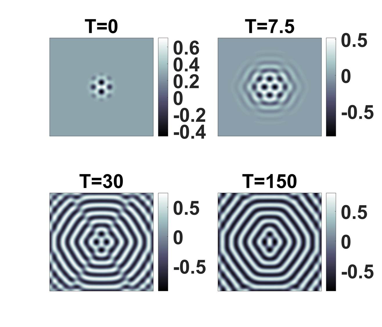 Figure 1
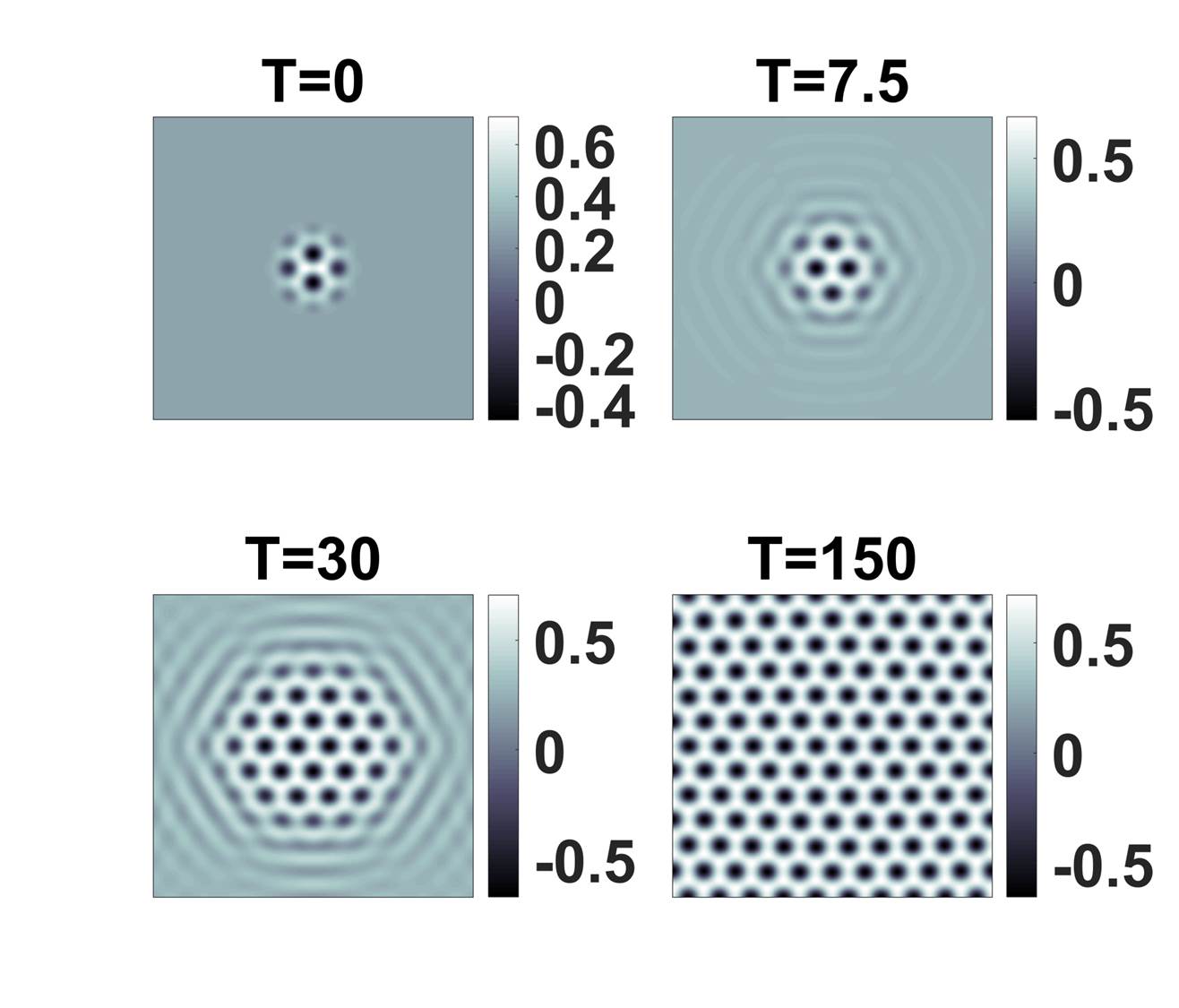 Figure 1
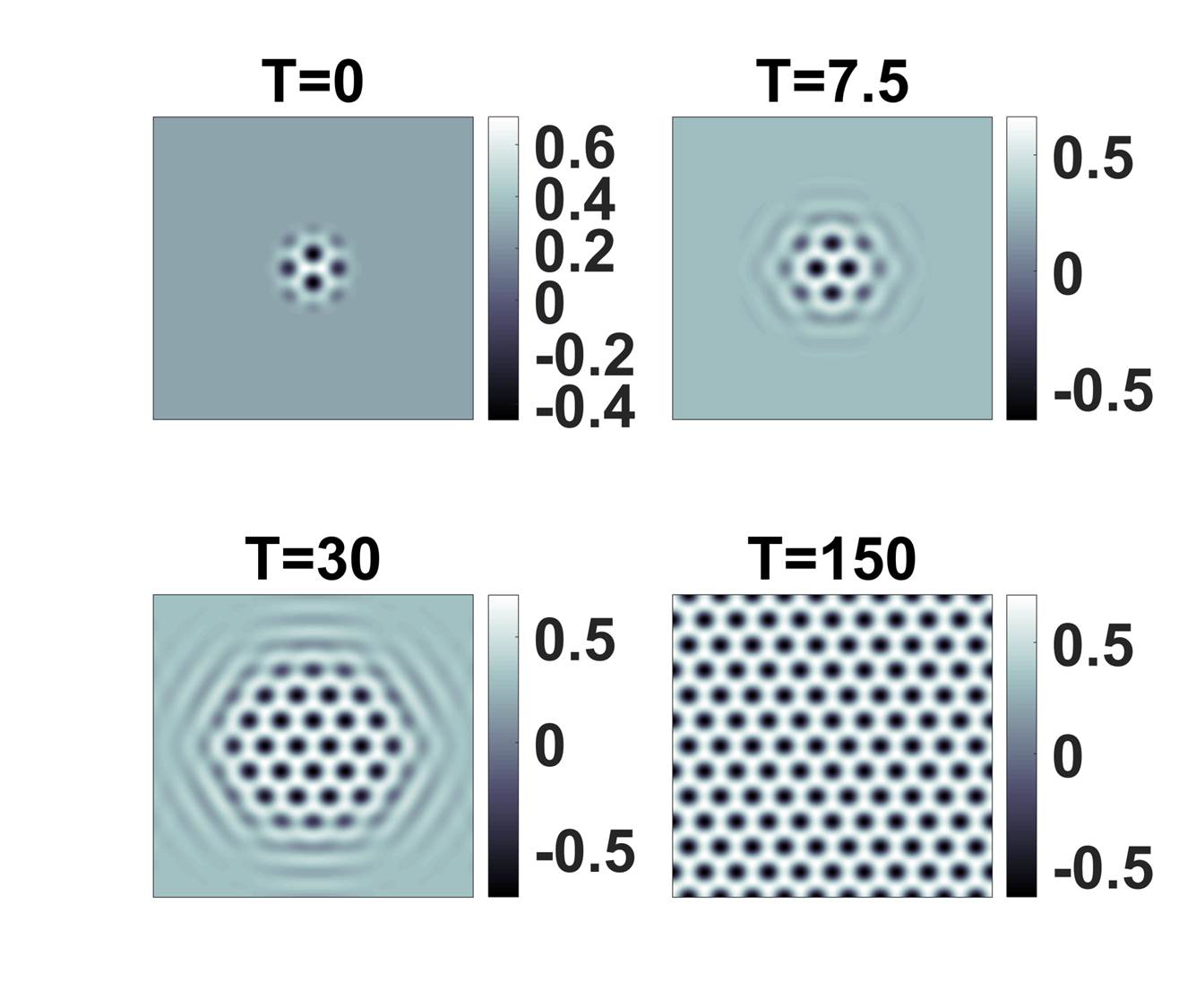 Figure 1
 Figure 1
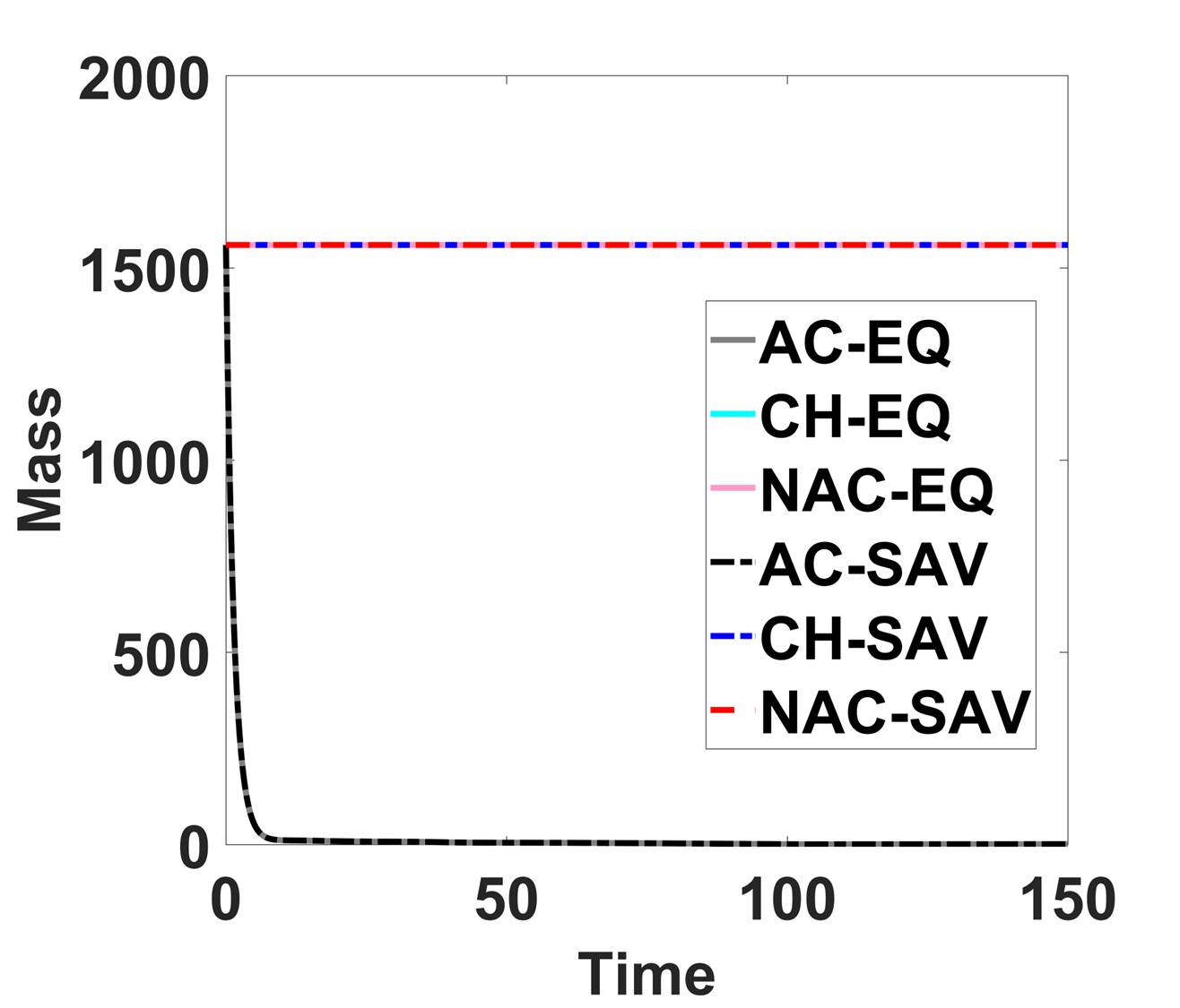 Figure 2
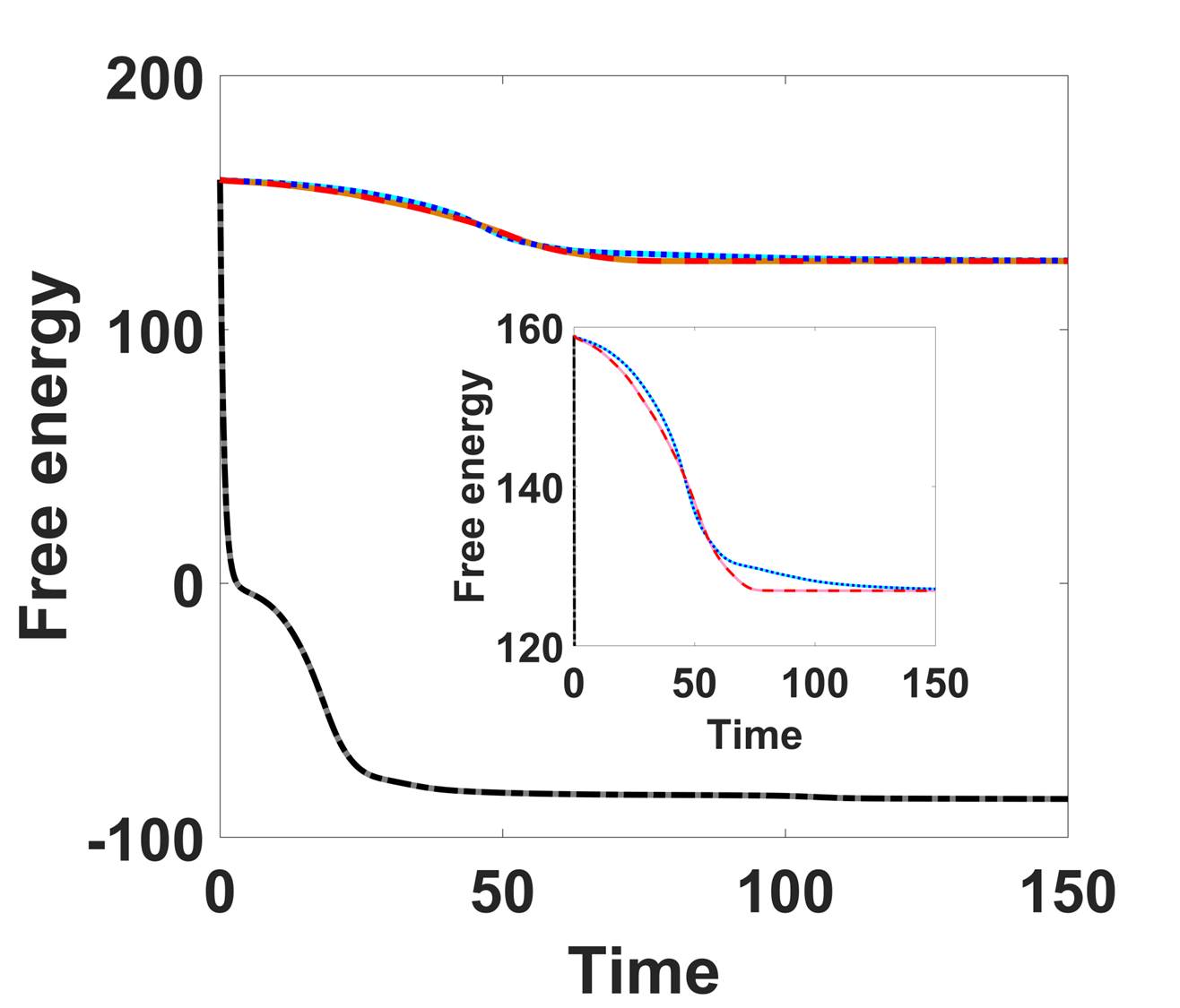 Figure 2
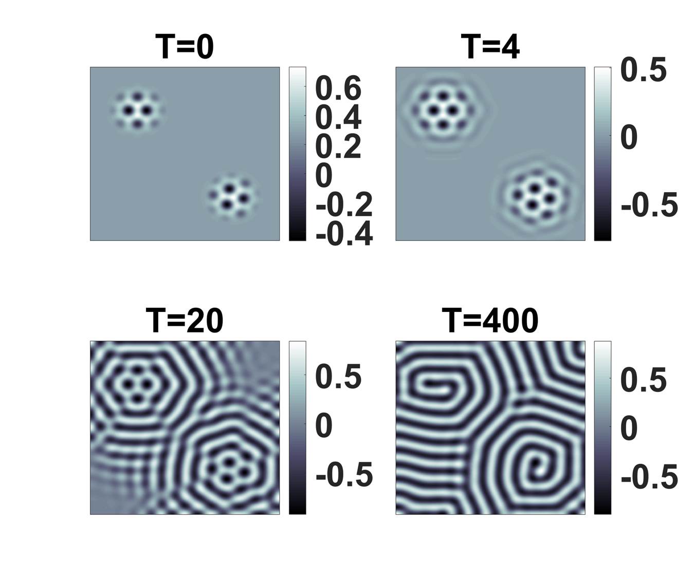 Figure 3
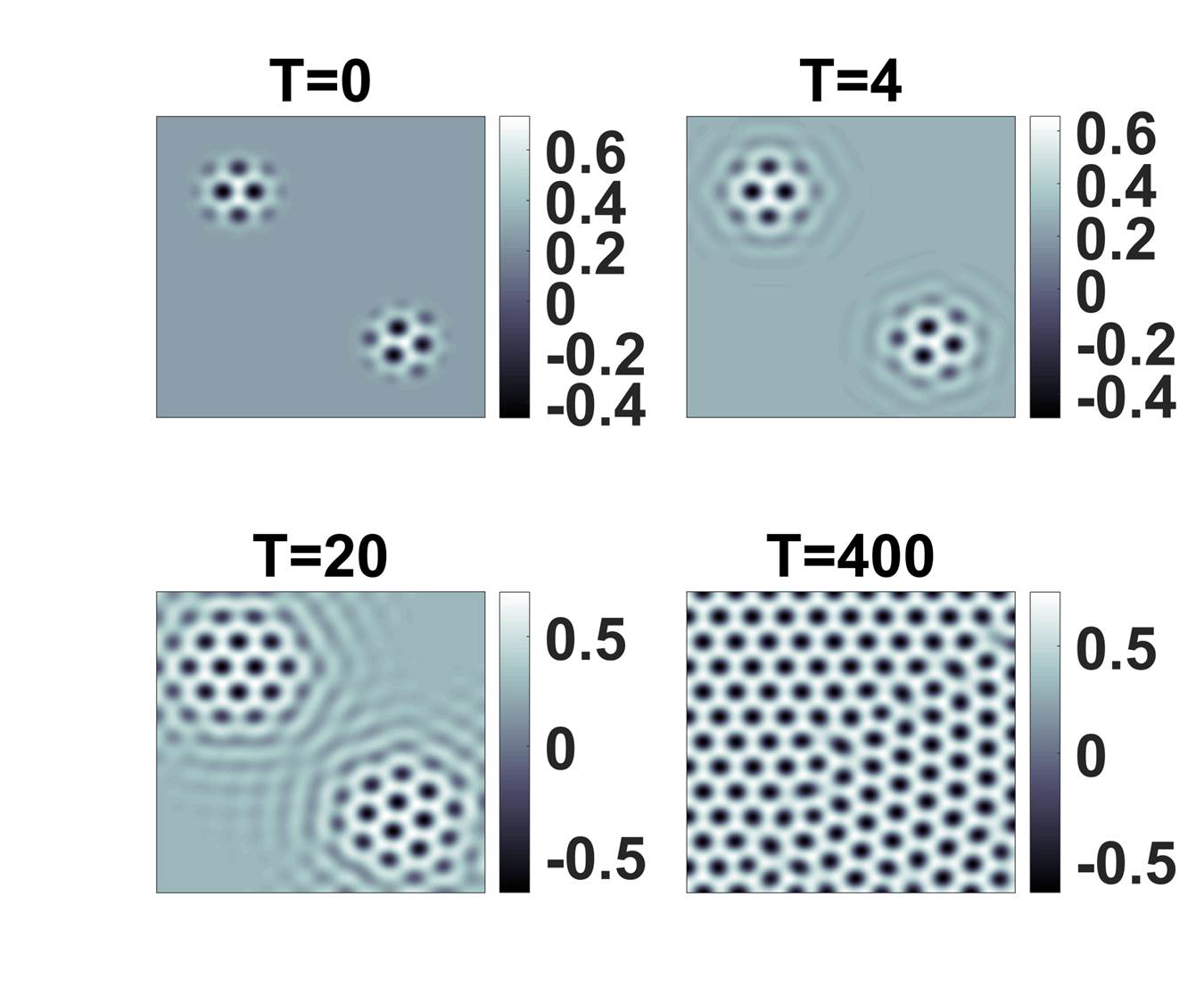 Figure 3
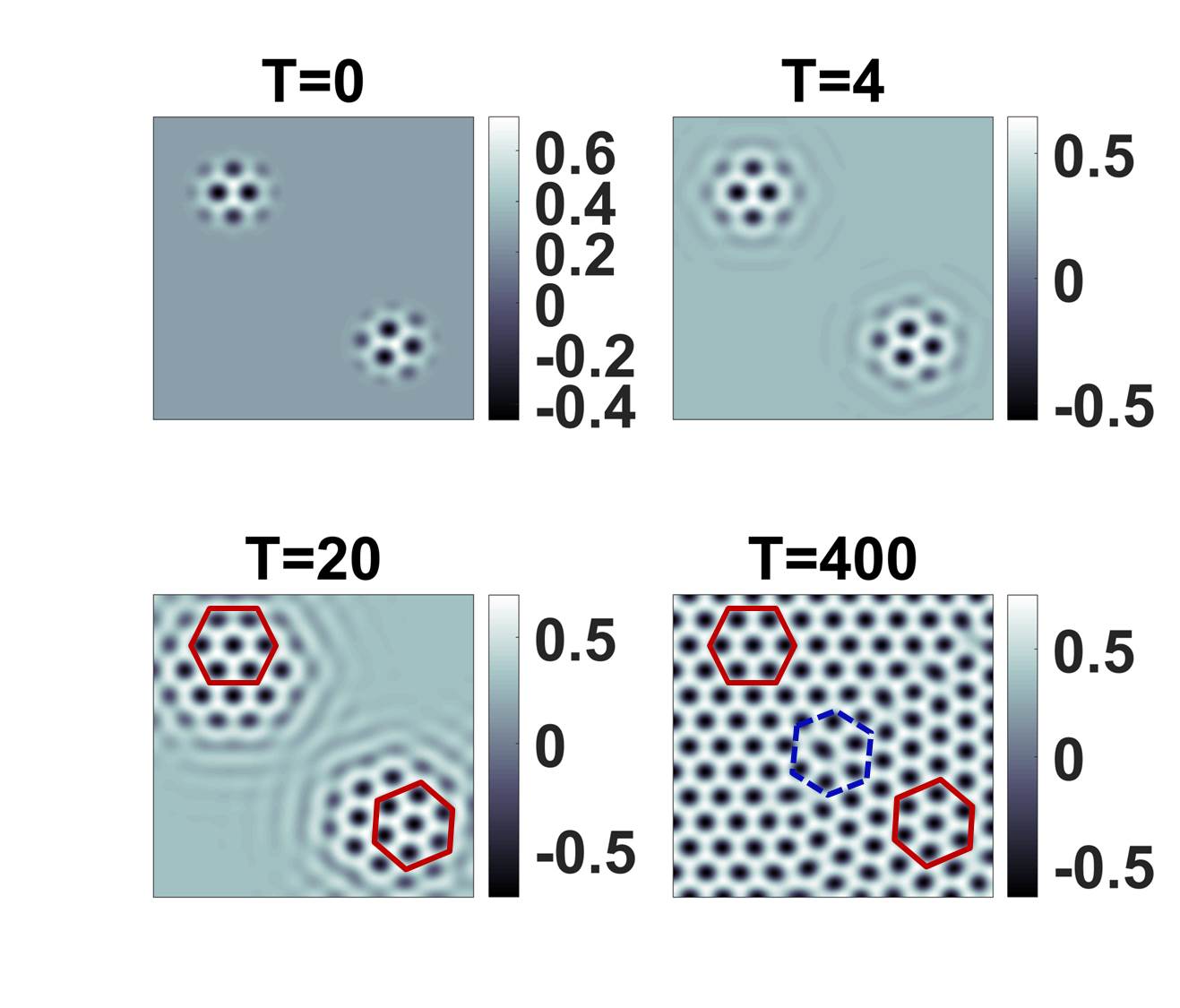 Figure 3
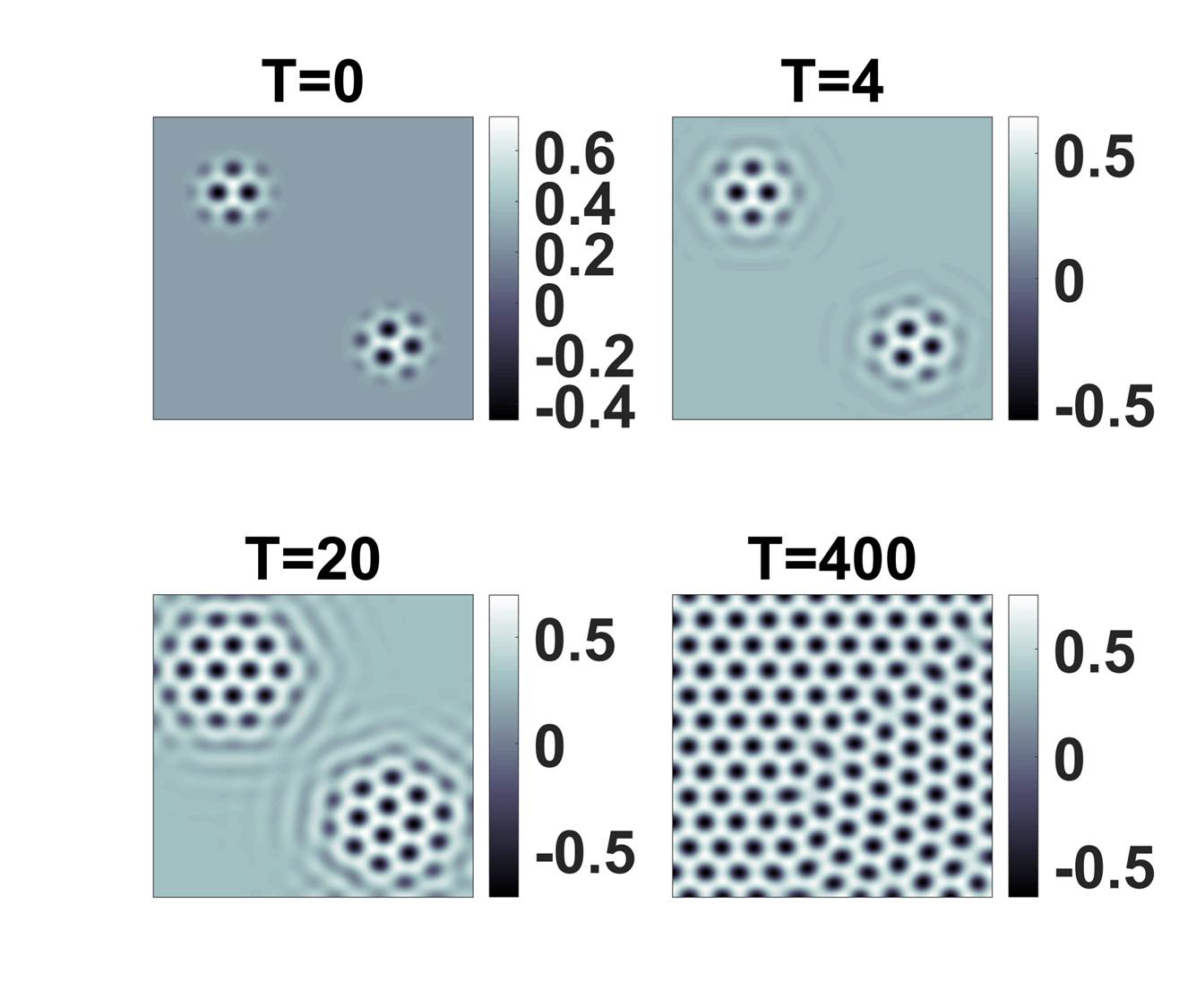 Figure 3
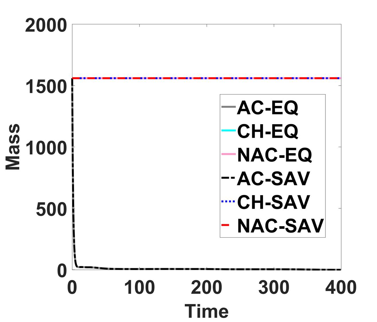 Figure 4
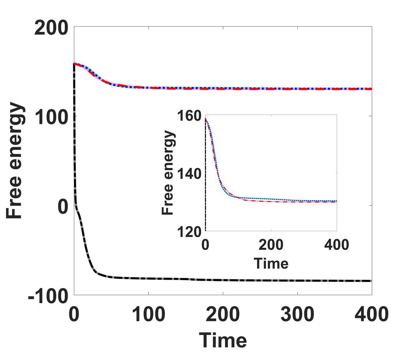 Figure 4
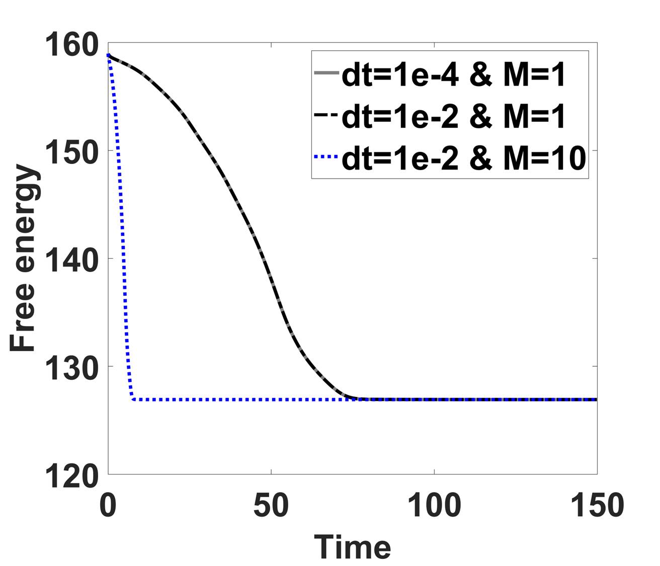 Figure 6
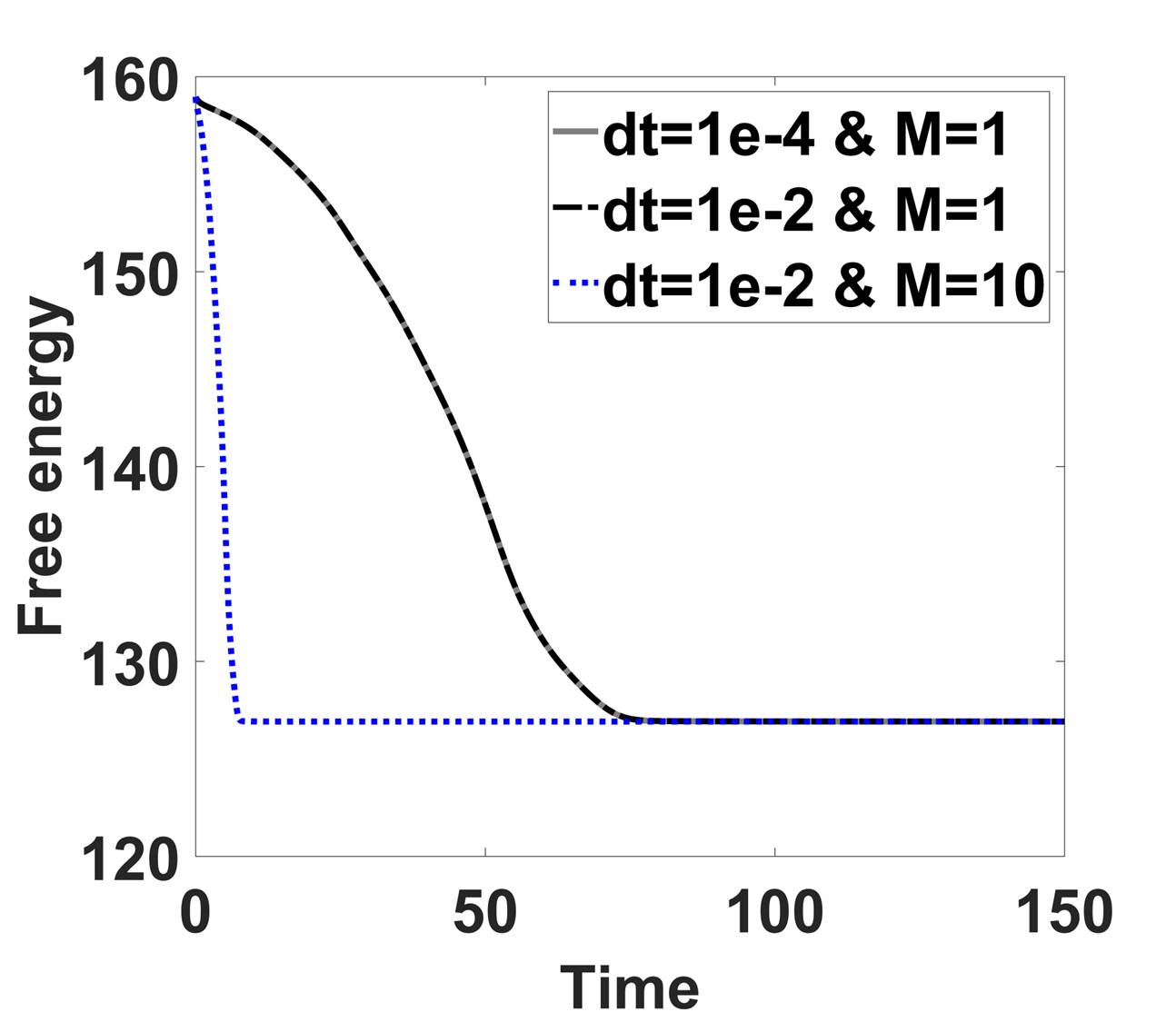 Figure 6
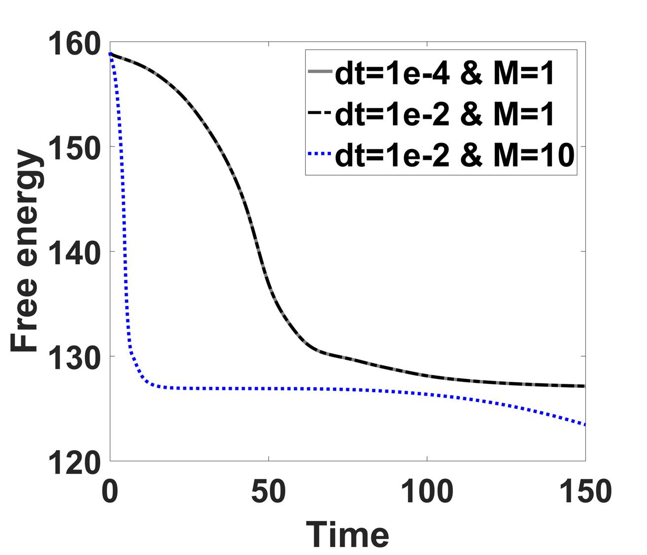 Figure 6
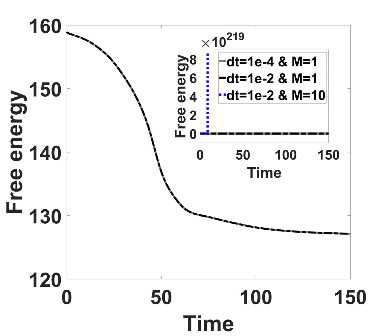 Figure 6
Peer Reviews
No public reviews on file for this paper yet. If you reviewed it on a platform where reviews are public (OpenReview, ICLR, NeurIPS, ICML), you can paste yours below so the community can read it here.
Videos
No videos yet. Explain this paper in a talk, walkthrough, or lecture? Add one.
Taxonomy
TopicsSolidification and crystal growth phenomena · Aluminum Alloy Microstructure Properties · nanoparticles nucleation surface interactions
Linear Second Order Energy Stable Schemes of Phase Field Model with Nonlocal Constraints for Crystal Growth
Xiaobo Jing0.10.10.1Beijing Computational Science Research Center, Beijing 100193, P. R. China. and Qi [email protected], Department of Mathematics, University of South Carolina, Columbia, SC 29028, USA; Beijing Computational Science Research Center, Beijing 100193, P. R. China.
Abstract
We present a set of linear, second order, unconditionally energy stable schemes for the Allen-Cahn model with a nonlocal constraint for crystal growth that conserves the mass of each phase. Solvability conditions are established for the linear systems resulting from the linear schemes. Convergence rates are verified numerically. Dynamics obtained using the nonlocal Allen-Cahn model are compared with the one obtained using the classic Allen-Cahn model as well as the Cahn-Hilliard model, demonstrating slower dynamics than that of the Allen-Cahn model but faster dynamics than that of the Cahn-Hillard model. Thus, the nonlocal Allen-Cahn model can be an alternative to the Cahn-Hilliard model in simulating crystal growth. Two Benchmark examples are presented to illustrate the prediction made with the nonlocal Allen-Cahn model in comparison to those made with the Allen-Cahn model and the Cahn-Hillard model.
Keywords: Allen-Cahn equation with nonlocal constraints, Phase field model,Crystal growth, Energy stable schemes, Energy quadratization.
1 Introduction
Phase field crystal (PFC) growth model, developed as an extension to the phase field formalism [12, 11, 35, 25, 27], has been successfully applied to various applications in materials science across different time scales [13, 34, 1], capturing the interaction between material defects [12] and modeling the microstructure evolution [12, 11, 13, 2, 3, 42, 22, 4, 29, 33]. It is a challenge to develop efficient and stable numerical algorithms to faithfully simulate dynamics described by the PFC model. The PFC model is thermodynamically consistent in that the free energy of the thermodynamic model is dissipative. Numerical algorithms that respect the free energy dissipation property at the discrete level are known as energy stable schemes.
The Cahn-Hilliard equation is a popular phase field model for crystal growth because of its mass (or volume) preserving property. However, the Cahn-Hilliard equation for the crystal growth problem is of up to the 6th order spatial derivative. Searching for a lower order phase field model that can also preserve mass and free energy dissipation properties is therefore a viable alternative. Allen-Cahn equation is a popular phase field model which normally has lower spatial derivatives than the Cahn-Hilliard model. It describes relaxation dynamics of the thermodynamical system to equilibrium. However, in the case of a phase field description, when the phase variable represents the mass fraction or the volume fraction of a material component, this model does not warrant the conservation of mass of that component. In order to conserve mass, the free energy functional has to be augmented by a mass preserving penalty term or with a Lagrange multiplier [30, 49, 36, 28, 10]. This thus modifies the Allen-Cahn equation into a nonlocal equation. We call this the nonlocal Allen-Cahn model or the Allen-Cahn model with a nonlocal constraint. Rubinstein and Sternberg studied the Allen-Cahn model with a mass constraint analytically and compared it with the Cahn-Hilliard model [36]. Their result seems to favor using the Allen-Cahn model with a mass constraint in place of the Cahn-Hilliard model when studying interfacial dynamics of incompressible, immiscible multi-component material systems.
For the classical Allen-Cahn equation as well as the Cahn-Hilliard equation, there have been several popular numerical approaches to construct energy stable schemes for the equations, including the convex splitting approach [14, 17, 16, 47, 37, 45, 23] , the stabilizing approach [40, 9, 7], the energy quadratization (EQ) approach [57, 52, 21, 20] and the scalar auxiliary variable approach [39, 8, 46]. Recently, the energy quadratization (EQ) and its reincarnation in the scalar auxiliary variable (SAV) method have been applied to a host of thermodynamic and hydrodynamic models owing to their simplicity, ease of implementation, computational efficiency, linearity, and most importantly their energy stability property [53, 52, 21, 20, 51, 54, 55, 6, 48, 58, 56, 59, 8, 46]. Ones have shown that these strategies are general enough to be useful for developing energy stable numerical approximations to any thermodynamically consistent models, i.e., the models satisfy the second law of thermodynamics or are derived from the Onsager principle [31, 32, 57]. The convex splitting approach, scalar auxiliary variable, energy quadratization approach and other methods have been applied to the Cahn-Hillard model for crystal growth [44, 47, 38, 57, 50, 24, 15, 19, 18, 41, 43].
In this paper, we develop a set of linear, second order, unconditionally energy stable schemes using the energy quadratization (EQ) and scalar auxiliary variable (SAV) approach to solve the nonlocal Allen-Cahn equation numerically. The numerical schemes for the Allen-Cahn and the Cahn-Hilliard model are recalled in the paper simply for comparison purposes. In some of these schemes, both EQ and SAV methods are combined to yield linear, energy stable schemes. We note that when a nonlocal Allen-Cahn model is discretized, it is inevitable to yield an integral which has to be treated with a scalar auxiliary variable. When multiple integrals are identified as SAVs in the free energy functional of the Allen-Cahn model with nonlocal constraints, new solution procedures are developed to solve the subproblems in which elliptic equations can be solved efficiently. All these schemes are linear and second order accurate in time. On the other hand,when the EQ strategy is coupled with the discretized integrals, the Sherman-Morrison formula can lead us to an efficient numerical scheme as well. In fact, this can be equivalently dealt with using the SAV method, which will be discussed in the Appendix. The numerical schemes developed in this study for the Allen-Cahn equation with nonlocal constraints preserve not only mass but also the energy dissipation rate at the discrete level.
In the end, we conduct two numerical experiments to assess the performance of the schemes. The results based on EQ and those based on SAV methods perform equally well in preserving mass and the energy dissipation rate. In addition, the computational efficiency of the schemes is comparatively studied in one of the benchmark examples as well. To simplify the presentation, we present the temporal discretization of the models using EQ and SAV approaches in detail. Then, we only briefly discuss the strategy to obtain fully discrete schemes by discretizing the semi-discrete schemes in space later. We refer readers to our early publications in [21, 20] for details. We show that the linear systems resulting from the schemes are all solvable uniquely if the time step size is suitable so that the solution existence and uniqueness in the full-discrete system is warranted.
The rest of the paper is organized as follows. In , we present the mathematical models for the classical Allen-Cahn, the Cahn-Hilliard, and the Allen-Cahn model with nonlocal constraints. In , we compare their near equilibrium dynamics. In , we present a set of second order, linear, energy stable numerical schemes for the models. In , we conduct mesh refinement tests on all the schemes and carry out two simulations on crystal growth as well as its grain-boundary effects using the models. Finally, we give the concluding remark in section .
2 Phase Field Models for Crystal Growth
We consider a phase field model for modeling crystal growth in solids with a focus on resolving the detail of transient dynamics. The free energy of the phase field model for crystal growth is given by [11, 25, 19]
[TABLE]
where represents an atomistic density field, which is the deviation of the density from the average density and is a conserved field variable, is a parameter related to the temperature, that is, higher corresponds to a lower temperature, and is the gradient operator ( denotes the Laplacian). In this study, we use a more general form of the free energy given by
[TABLE]
where recovers equation (2.2) and the boundary conditions
[TABLE]
are assumed.
Based on the Onsager linear response theory[31, 32], transient dynamics of such a system is customarily governed by a time-dependent partial differential equation given by
[TABLE]
subject to appropriate boundary and initial conditions, where and are the mobility matrix and the chemical potential, respectively.
The time rate of change of the free energy is given by
[TABLE]
The following boundary conditions will annihilate the boundary terms in the energy dissipation functional
[TABLE]
In the crystal growth model, . So, the boundary conditions reduce to
[TABLE]
This set of boundary conditions is consistent with the derivation of the free energy functional.
An alternative set of boundary conditions is given by
[TABLE]
This is equivalent to
[TABLE]
This is different from the previous one.
We can also assign dissipative boundary conditions to the model as follows
[TABLE]
where is inversely proportional to a relaxation time. The boundary contribution to the energy dissipation is then given by
[TABLE]
The total energy dissipation rate or energy dissipation functional is given by
[TABLE]
If , we recover (2.15).
Two well-known phase field models are the Allen-Cahn and the Cahn-Hilliard equation, whose mobility is given respectively by
[TABLE]
where is a prescribed mobility coefficient matrix, which can be a function of . The Allen-Cahn equation does not conserve the total mass if is the mass-fraction while the Cahn-Hilliard equation does. However, these two models predict similar near equilibrium dynamics. On the other hand the Allen-Cahn equation is an equation of lower spatial derivatives, and presumably costs less when solved numerically. Thus, one can impose the mass conservation as a constraint to the Allen-Cahn equation for it to be used to describe dynamics in which the mass is conserved. Next, we will briefly recall several ways to enforce mass conservation to dynamics described by the Allen-Cahn equation.
2.1 Allen Cahn model
The classical Allen-Cahn equation with the non-flux Neumann boundary conditions is given by
[TABLE]
where is the mobility coefficient and is the chemical potential
[TABLE]
The energy dissipation rate of the Allen-Cahn equation is given by
[TABLE]
provided nonnegative . The Allen-Cahn model does not conserve the mass if the mass is denoted as .
2.2 Cahn-Hillard model
The Cahn-Hilliard equation with the non-flux Neumann boundary condition is given by
[TABLE]
where is the mobility coefficient and is the chemical potential
[TABLE]
The energy dissipation rate of the equation is given by
[TABLE]
provided nonnegative . The Cahn-Hillard model conserves the mass. We next discuss the nonlocal Allen-Cahn equation that conserves the mass.
2.3 Nonlocal Allen-Cahn models
we present two methods to impose mass conservation. One is called the Allen-Cahn model with a penalizing potential and the other is called the Allen-Cahn model with a Lagrange multiplier.
2.3.1 Allen-Cahn model with a penalizing potential
In the Allen-Cahn model with a penalizing potential model, a penalizing term is augmented to the free energy to enforce the mass conservation by the model as follows
[TABLE]
where is penalizing parameter, is the initial mass.
The transport equation for is given by the Allen-Cahn equation
[TABLE]
where is the mobility coefficient and is the chemical potential given by
[TABLE]
We calculate the energy dissipation rate as follows
[TABLE]
provided . The modified Allen-Cahn equation is approximately mass preserving depending on the size of and nonlocal. We next discuss another approaches to obtain a nonlocal Allen-Cahn model.
2.3.2 Allen-Cahn model with a Lagrange multiplier
In this model, the free energy is augmented by a penalty term with a Lagrange multiplier as follows.
[TABLE]
The transport equation for is given by the Allen-Cahn equation
[TABLE]
where is the mobility coefficient and is the chemical potential given by
[TABLE]
We calculate the energy dissipation rate as follows
[TABLE]
provided .
3 Near equilibrium dyamics of the models
We study dynamics of the models near their equilibrium solution . We consider a small perturbation of the steady state given by :
[TABLE]
For the Allen-Cahn model, substituting (3.2) into (2.27), we get
[TABLE]
We seek the solution of the linearized partial differential equation system given by
[TABLE]
in the domain . Then, we have
[TABLE]
Instability can emerge if , for some wave numbers , .
For the Allen-Cahn model with a penalizing potential, substituting (3.2) into the transport equation, we obtain the linearized system as follows
[TABLE]
Using the ansatz (3.5), we have
[TABLE]
If , instability will occur. In comparison, the Allen-Cahn model with a penalizing potential is more stable than the classical Allen-Cahn model.
For the Allen-Cahn model with a Lagrange multiplier, substituting equation 3.2 into the transport equation, we get the linearized system
[TABLE]
where . Solving the linear system using ansatz (3.5), we have
[TABLE]
If , instability may ensure. The contribution of the Lagrange multiplier is to introduce a destabilizing mechanism depending on steady state solution .
For the Cahn-Hillard model, repeating the above analysis, we have the dynamical equation for the Fourier coefficients:
[TABLE]
The window of instability in the Cahn-Hillard model is identical to that in the Allen-Cahn model. However, the growth rates differ.
The linear stability results dictate initial transient dynamics of the solution towards or away from the given steady state. We will resort to numerical computations for long time transient behavior of the solution.
4 Numerical Approximations to the Phase Field Models
We design numerical schemes to solve the above nonlocal phase field equations to ensure that the energy dissipation property as well as mass conservation are respected. We do it by employing the energy quadratization (EQ) and the scalar auxiliary variable method (SAV) developed recently [54, 58, 39, 48]. Both methods depend on a reformulation of the models into equivalent ones with a quadratic energy. From the latter, we have effective ways to design linear numerical schemes. For a full review on EQ methods for thermodynamical models, readers are referred to a recent review article [57]. All schemes presented below are firstly given as semi-discretized ones in time and then the full discretization in space will be discussed. In fact, we have shown recently that BDF and Runge-Kutta methods can be used to design energy stable schemes for thermodynamical systems up to arbitrarily high order in time [53]. For comparison purposes, we also present analogous schemes for the classical Allen-Cahn and the Cahn Hilliard model as well.
4.1 Temporal discretization
4.1.1 Numerical methods for the Allen-Cahn model by EQ methods
We reformulate the free energy density by introducing an intermediate variable:
[TABLE]
Then, the free energy recast into
[TABLE]
We rewrite (2.27) as
[TABLE]
where
[TABLE]
We now discretize it using the linear Crank-Nicolson method in time to arrive at a second order semi-discrete scheme.
Scheme 4.1**.**
Given initial conditions , we first compute by a first order scheme. Having computed , and , we compute as follows.
[TABLE]
where
[TABLE]
The numerical implementation can be done as follows
[TABLE]
where . So, is solved independent of .
We define the discrete energy as follows
[TABLE]
4.1.2 Numerical methods for the Allen-Cahn model by SAV methods
Introducing an intermediate variable as the scalar auxiliary variable, the free energy recast into
[TABLE]
We rewrite (2.27) as
[TABLE]
We then discretize it using the linear Crank-Nicolson method in time to arrive at a second order semi-discrete scheme.
Scheme 4.2**.**
Given initial conditions , we first compute by a first order scheme. Having computed , and , we compute as follows.
[TABLE]
where
[TABLE]
We define the discrete energy as follows
[TABLE]
The numerical scheme can be recast into
[TABLE]
where and . Multiplying the inverse of firstly and taking the inner product of the equation with c secondly, we have
[TABLE]
Then, the solution in the scheme is solved in the following steps,
[TABLE]
4.1.3 Numerical methods for the Cahn-Hillard model by EQ methods
The free energy density is reformulated by introducing an intermediate variable:
[TABLE]
Then, the free energy recast into
[TABLE]
We rewrite (2.35) as
[TABLE]
where
[TABLE]
We then discretize it using the linear Crank-Nicolson method in time to arrive at a second order semi-discrete scheme.
Scheme 4.3**.**
Given initial conditions , we first compute by a first order scheme. Having computed , and , we compute as follows.
[TABLE]
The discrete energy is defined as follows
[TABLE]
The numerical implementation can be done as follows
[TABLE]
where .
4.1.4 Numerical methods for the Cahn-Hillard model by SAV methods
An intermediate variable are introduced to reformulate the free energy, which is
[TABLE]
We rewrite (2.35) as
[TABLE]
Linear Crank-Nicolson method is used in time to arrive at a second order semi-discrete scheme.
Scheme 4.4**.**
Given initial conditions , we first compute by a first order scheme. Having computed , and , we compute as follows.
[TABLE]
where
[TABLE]
The discrete energy is defined as follows
[TABLE]
The numerical scheme can be rewritten into
[TABLE]
where and . Multiplying the first equation by the inverse of firstly and taking the inner product of the equation with c secondly, we have
[TABLE]
So we solve the solution in the scheme in the following steps,
[TABLE]
4.1.5 Numerical method for the Allen-Cahn model with a penalizing potential by EQ methods
In the Allen-Cahn model with a penalizing potential, we reformulate the free energy density by introducing two intermediate variables
[TABLE]
Then, the free energy recast into
[TABLE]
We rewrite the nonlocal Allen-Cahn equation as follows:
[TABLE]
where
[TABLE]
We then discretize it using the linear Crank-Nicolson method in time to arrive at a new scheme as follows.
Scheme 4.5**.**
Given initial conditions , we first compute by a first order scheme. Having computed , and , we compute as follows.
[TABLE]
where
[TABLE]
The discrete energy is defined as follows
[TABLE]
From the scheme, it follows that
[TABLE]
It can be written into a compact form,
[TABLE]
where and
Then, the solve is solved in the following steps,
[TABLE]
4.1.6 Numerical method for the Allen-Cahn model with a penalizing potential by SAV methods
In the penalizing nonlocal Allen-Cahn model, we reformulate the free energy density by introducing two intermediate variables
[TABLE]
Then, the free energy recast into
[TABLE]
We rewrite the nonlocal Allen-Cahn equation as follows:
[TABLE]
where
[TABLE]
We then discretize it using the linear Crank-Nicolson method in time to arrive at a new scheme as follows.
Scheme 4.6**.**
Given initial conditions , we first compute by a first order scheme. Having computed , and , we compute as follows.
[TABLE]
where
[TABLE]
The discrete energy is defined as follows
[TABLE]
The scheme can be recast into
[TABLE]
where
[TABLE]
It implies that
[TABLE]
We solve for and from the above equation after we obtain
[TABLE]
So, the solution is solved in the following steps,
[TABLE]
4.1.7 Numerical method for the Allen-Cahn model with a Lagrange multiplier by EQ methods
We reformulate the free energy density by introducing an intermediate variable
[TABLE]
Then, the free energy recast into
[TABLE]
We rewrite (2.54) as
[TABLE]
where
[TABLE]
We then discretize it using the linear modified Crank-Nicolson method in time as follows.
Scheme 4.7**.**
Given initial conditions , we first compute by a first order scheme. Having computed , and , we compute as follows.
[TABLE]
where
[TABLE]
Remark: .
Then, we have the following theorem
Theorem 4.1**.**
The mass of each phase is conserved, i.e.,
[TABLE]
Proof: Substituting the into the equation below, we have
[TABLE]
This implies the masse-conservation property.
We define the discrete energy as follows
[TABLE]
The solution is solved in the following steps
[TABLE]
where
[TABLE]
4.1.8 Numerical method for the Lagrangian models by SAV methods
We reformulate the free energy density by introducing an intermediate variable
[TABLE]
Then, the free energy recast into
[TABLE]
We rewrite (2.54) as
[TABLE]
where
[TABLE]
We then discretize it using the modified Crank-Nicolson method in time as follows.
Scheme 4.8**.**
Given initial conditions , we first compute by a first order scheme. Having computed , and , we compute as follows.
[TABLE]
where
[TABLE]
Then, we have the following theorem
Theorem 4.2**.**
The mass of each phase is conserved, i.e.,
[TABLE]
Proof: The proof is similar to that of theorem 4.1 and is thus omitted.
We define the discrete energy as follows
[TABLE]
This scheme can be recast into
[TABLE]
So we have
[TABLE]
We solve for and from the above equations after we obtain
[TABLE]
where
[TABLE]
Finally, the solution is obtained as follows
[TABLE]
4.2 Spatial discretization
We use the finite difference method to discretize the equations with the Neumann boundary condition in space for all models. The linear spatially dependent PDE systems resulting from all semi-discrete schemes are spatially discretized by compact second order finite difference methods at the cell center. We divide the 2D domain into rectangular meshes with mesh sizes and , where , are two positive real numbers and , are the number of meshes in each direction. After this, the sets of the cell center points and for the uniform partition are defined as follows
[TABLE]
where and .
We define the east-west-edge-to-center and center-to-east-west-edge difference operators and as follows
[TABLE]
Similarly, we define the north-south-edge-to-center and center-to-north-south-edge difference operators and as follows
[TABLE]
The fully discrete Laplacian and fourth order gradient operator are given by
[TABLE]
The discrete inner product is defined as follows
[TABLE]
where and are given at the cell center. In particular,
[TABLE]
With the notations, we replace the continuous differential operators in the semi-discrete schemes by the discrete difference operators to arrive at the corresponding fully discrete schemes. To save space, we will not enumerate them here.
4.3 Energy dissipation property and solvability of the linear systems resulting from the schemes
We summarize the energy dissipation law and unique solvability for all linear systems resulting from the semidiscrete schemes presented in this section into two theorems. The proofs of the energy dissipation property and solvability for the fully discrete schemes are similar, we only prove the theorems for the Allen-Cahn model with a Lagrangian multiplier discreized using EQ methods below and omit others for simplicity. Based on scheme 4.7 and the spatial discretization, the fully discrete scheme corresponding to scheme 4.7 is summarized below.
Scheme 4.9**.**
Given initial conditions , we first compute by a first order scheme. Having computed , and , we compute as follows.
[TABLE]
where
[TABLE]
We define the discrete energy as follows
[TABLE]
Theorem 4.3**.**
The fully discrete scheme obeys the following energy dissipation law
[TABLE]
Proof: Taking inner product of (4.222) with , we obtain
[TABLE]
Taking inner product of with , we have
[TABLE]
Taking inner product of with , we obtain
[TABLE]
Combining the above equations, we obtain
[TABLE]
Substituting the expression of into the equation, we have
[TABLE]
Remark: (i). This proof applies to the semi-discrete schemes as well. (ii). When the linear schemes of the nonlocal Allen-Cahn model involve integrals discretized by a composite Trapezoidal rule, efficient numerical methods can be devised to solve the resulting linear systems. Such methods are derived from the Sherman-Morisson formula (See Appendix).
Theorem 4.4**.**
The linear system resulting from the above fully discrete scheme admits a unique solution.
Proof: Note that the solution in scheme 4.222 is solved via the following steps
[TABLE]
where
[TABLE]
From the Sherman-Morrison formula, we notice that the solution uniqueness of depends on the uniqueness of the corresponding linear system . Now we only need to prove the uniqueness of the solution for
[TABLE]
If is small enough, we have
[TABLE]
So, has only zero solution.
Remark: One can prove the uniqueness of the solution for any time step size if in equation (4.222).
5 Numerical Results and Discussions
In this section, we conduct mesh refinement tests to validate the accuracy of the proposed schemes and then present some numerical examples to assess the schemes for the nonlocal Allen-Cahn models against those for the Cahn-Hilliard model. For convenience, we refer the numerical schemes designed by EQ methods for the Allen-Cahn model, the Cahn-Hilliard model, the Allen-Cahn model with a penalizing potential and the Allen-Cahn model with a Lagrangian multiplier as AC-EQ, CH-EQ, AC-P-EQ and AC-L-EQ, respectively. Similarly, we name the numerical schemes obtained using SAV approaches for the models as AC-SAV, CH-SAV, AC-P-SAV, AC-L-SAV, respectively. In the following, we set the constant in the free energy at in all computations.
5.1 Accuracy test
We confirm the convergence rates of the proposed schemes for the PFC models through mesh refinement tests. The computational domain is set as . The model parameter values are chosen as . We solve the equations with the initial condition given by
[TABLE]
We choose the space step size . By taking a linear refinement path , , we calculate the errors of the phase variable with adjacent k at . The tables show the schemes are second order accurate in time numerically.
We also compare the computational efficiency of all schemes designed by EQ and SAV methods with and in table 3. The AC-P-EQ/SAV schemes perform the best among the schemes for nonlocal Allen-Cahn models. Besides this, AC-P-EQ/SAV schemes also perform better than CH-EQ/SAV schemes in most test cases. In fact, the accuracy of the Cahn-Hillard model relies on the mobility coefficient more sensitively than the Allen-Cahn models do. Hence, the accuracy of the schemes for the nonlocal Allen-Cahn models is better than that for the Cahn-Hillard model if is large. We will discuss it in more details next (see Figure 5.5).
Table 1 Mesh refinement tests for the proposed schemes using EQ methods.
Scheme AC-EQ CH-EQ AC-P-EQ AC-L-EQ
Coarse Fine error order error order error order error order
5.00E-02 2.5E-2 1.21E-06
1.23E-05
1.21E-06
1.21E-06
2.5E-2 1.25E-2 3.02E-07 2.00 3.12E-06 1.98 3.02E-07 2.00 3.02E-07 2.00
1.25E-2 6.25E-3 7.56E-08 2.00 7.84E-07 1.99 7.56E-08 2.00 7.56E-08 2.00
6.25E-3 3.125E-3 1.89E-08 2.00 1.96E-07 2.00 1.89E-08 2.00 1.89E-08 2.00
3.125E-3 1.5625E-3 4.72E-09 2.00 4.90E-08 2.00 4.72E-09 2.00 4.72E-09 2.00
Table 2 Mesh refinement tests for the proposed schemes using SAV methods.
Scheme AC-SAV CH-SAV AC-P-SAV AC-L-SAV
Coarse Fine error order error order error order error order
5.00E-02 2.5E-2 1.24E-06
1.22E-05
1.24E-06
1.24E-06
2.5E-2 1.25E-2 3.09E-07 2.00 3.10E-06 1.98 3.09E-07 2.00 3.09E-07 2.00
1.25E-2 6.25E-3 7.72E-08 2.00 7.78E-07 1.99 7.72E-08 2.00 7.72E-08 2.00
6.25E-3 3.125E-3 1.93E-08 2.00 1.95E-07 2.00 1.93E-08 2.00 1.93E-08 2.00
3.125E-3 1.5625E-3 4.83E-09 2.00 4.87E-08 2.00 4.82E-09 2.00 4.82E-09 2.00
Table 3 Efficiency of the schemes at time steps with respect to and (From top to below).
Scheme AC-EQ AC-SAV CH-EQ CH-SAV AC-P-EQ AC-P-SAV AC-L-EQ AC-L-SAV
Time (s) 45.3 77.9 66.0 107.8 68.3 90.0 110.0 103.2
Time (s) 44.4 76 54.6 104 38.8 84.2 53.9 100.7
Time (s) 53.4 75.0 66.8 111.9 61.4 83.2 103.3 99.5
5.2 Assessment of the numerical schemes
To further assess the numerical schemes, we numerically solve the model equations using the schemes with respect to two benchmark problems. Firstly we simulate the phase transition of crystal growth in 2D. We use time step and space mesh in the 2D simulation. A solid crystallite with Hexagonal ordering in 2D is initially placed in the centre of the domain, which is assigned an average density . The initial condition is given by
[TABLE]
where
[TABLE]
[TABLE]
is the center coordinate of the domain, and is of the domain length in the x-direction. The domain is given by , and . The other values are and
Figure 5.1 shows time evolution of the crystal growth process computed by AC-EQ, CH-EQ, AC-P-EQ and AC-L-EQ schemes, respectively. In Figure 5.1-(a), the crystal growth simulated by the Allen-Cahn model can’t preserve the Hexagonal ordering, different from the results simulated by the Cahn-Hillard model in Figure 5.1-(b) and the nonlocal Allen-Cahn models in Figure 5.1-(c) and (d). The time evolution of mass and free energy are shown in Figure 5.2-(a) and (b) respectively. The results computed by the EQ and SAV schemes for the same model (Allen-Cahn model, Cahn-Hillard model and nonlocal Allen-Cahn model) are identical. We don’t see any differences between the results of the Allen-Cahn model with a penalizing potential and the Allen-Cahn model with a Lagrangian multiplier either. The mass decays in the Allen-Cahn model to nearly zero in finite time. In contrast, the mass in the Cahn-Hillard model and the nonlocal Allen-Cahn models is conserved in the simulations. Meantime, the free energies of the Cahn-Hillard model and the nonlocal Allen-Cahn models are larger than that of the Allen-Cahn model. Figure 5.2-(b) shows that the free energy computed by the nonlocal Allen-Cahn model reaches the steady state faster than that of the Cahn-Hillard model.
Secondly we simulate another case of polycrystalline growth involving the grain boundary effect, where the two initial crystallites with a hexagonal configuration oriented in different direction (or misorientation) are put in the domain. Grain boundaries appear when the two crystals meet during the growth, which yields some orientation mismatch. The initial condition is given by
[TABLE]
where
[TABLE]
, and is the center of the domain. The other parameters and the domain are the same as in the first example. By doing an affine transformation of the Cartesian coordinates to produce a rotation in the domain, the modified coordinates can be used to generate the crystallites in different directions,
[TABLE]
We put two crystallites in the domain, the first one is defined as equation (5.15) with , the other is with
Figure 5.3 depicts the grain boundary effect during polycrystalline growth computed by AC-SAV, CH-SAV, AC-P-SAV and AC-L-SAV schemes, respectively. The snapshots of the phase transitions computed by the Cahn-Hillard and the nonlocal Allen-Cahn models show the Hexagonal ordering are broken at the center at . The time evolution of mass and free energy are shown in Figure 5.4-(a) and (b), respectively. The mass in the Allen-Cahn model decays in time. In contrast, the mass in the Cahn-Hillard model and the nonlocal Allen-Cahn models are conserved during the simulation. Meanwhile, the free energies in the Cahn-Hillard model and the nonlocal Allen-Cahn models are larger than that of the Allen-Cahn model. In Figure 5.4-(b), the nonlocal Allen-Cahn models and the Cahn-Hillard model predict comparable time evolution of the free energy but the nonlocal Allen-Cahn models reach the steady state first. The results computed by the EQ and SAV schemes for the same model (the Allen-Cahn model, Cahn-Hillard model and nonlocal Allen-Cahn model) are nearly identical. We don’t see any differences between the results of the Allen-Cahn model with a penalizing potential and the Allen-Cahn model with a Lagrangian multiplier either.
We note that the results computed by the Allen-Cahn model with a penalizing potential and the Allen-Cahn model with a Lagrangian multiplier in the above two examples at are the same. However, the choice of can certainly affect the outcome. In principle, should be chosen as large as possible. However, when is too large, the governing equation becomes very stiff, which forces one to use extremely small time-step size in order to resolve the detail correctly. On the other hand, as we have shown in the two examples, is good enough to produce the results that conserve mass very well.
Both Figure 5.2 and Figure 5.4 show that the free energy computed by the nonlocal Allen-Cahn models reach the steady state faster than that of the Cahn-Hillard model, which is different from our previous results on a different free energy functional [26]. Especially, the simulations computed by the models with mobility coefficient and time steps show the same time evolution behavior. When the mobility is large, say , and , the CH-SAV produce an erroneous result while the others produce comparable ones. In practice, if the steady state is more important than the transition dynamics, one can enlarge the mobility coefficient of the models to accelerate the convergence to steady state. But, CH-SAV seems to have some accuracy issues with this approach. The results of the nonlocal Allen-Cahn models in 5.5-(a) and (b) show better performance than the Cahn-Hillard model dose in Figure 5.5-(c) and (d).
6 Conclusions
We have developed a set of linear, second order, energy stable schemes for the Allen-Cahn equation with nonlocal constraints that conserve mass and compared them with the energy stable, linear schemes for the Allen-Cahn and the Cahn-Hilliard model. These schemes are devised based on the energy quadratization strategy in the form of EQ and SAV formulation, respectively. We show that they are unconditionally energy stable and uniquely solvable. All schemes can be solved using efficient numerical methods, making the models alternatives to the Cahn-Hilliard model to describe interface dynamics of immiscible materials while conserving mass. The nonlocal Allen-Cahn models show a faster coarsening rate than that of the Cahn-Hilliard model at the same mobility, but one can enlarge the mobility coefficient of the nonlocal Allen-Cahn model to accelerate their dynamics in case only steady states are of interest. In addition, we have compared the two Allen-Cahn models with nonlocal constraints numerically. The computational efficiency of the Allen-Cahn model with a penalizing potential is slightly better than the one with a Lagrange multiplier, but the accuracy of the former depends on a suitable choice of model parameter . If the steady state is desired rather than the transient dynamical behavior, large time step size and mobility coefficient can be used to accelerate the simulation. In the end, we show that the nonlocal Allen-Cahn models perform better that the Cahn-Hilliard model in the case of a large time step and mobility coefficient.
Acknowledgements
Xiaobo Jing and Qi Wang’s research is partially supported by NSFC awards #11571032, #91630207 and NSAF-U1530401.
Appendix
Appendix A Shermann-Morrison formula and its application to solving integro-differential equations
Here we give a brief review over the Sherman-Morrison formula [5] and explain its applications in the practical implementation of our various relevant schemes.
Suppose is an invertible square matrix, and , are column vectors. Then is invertible iff . If is invertible, then its inverse is given by
[TABLE]
So if and , has the solution given by
[TABLE]
For the integral term(s) in the semi-discrete schemes in this study such as (4.150), we need to discretize it properly. , we discretize using the composite trapezoidal rule and adding all the elements of the new matrix , where , , , are the spatial step sizes and . For convenience, we use to represent the integral discretized by the composite trapezoidal rule.
To solve equation (4.150), we discretize the integral or the inner product of functions as . The scheme is recast to . After using the Sherman-Morrison formula, we get
[TABLE]
In the inner product of vectors, (4.150) can be rewritten into
[TABLE]
So, indeed the approach we take in the study using the discrete inner product is essentially equivalent to applying the Sherman-Morrison formula.
The reference list from the paper itself. Each links out to its DOI / PubMed record.
- 1[1] Ebrahim Asadi and Mohsen Asle Zaeem. A review of quantitative phase-field crystal modeling of solid–liquid structures. Jom , 67(1):186–201, 2015.
- 2[2] Rainer Backofen, Andreas Rätz, and Axel Voigt. Nucleation and growth by a phase field crystal (pfc) model. Philosophical Magazine Letters , 87(11):813–820, 2007.
- 3[3] Rainer Backofen and Axel Voigt. A phase-field-crystal approach to critical nuclei. Journal of Physics: Condensed Matter , 22(36):364104, 2010.
- 4[4] Joel Berry, KR Elder, and Martin Grant. Simulation of an atomistic dynamic field theory for monatomic liquids: Freezing and glass formation. Physical Review E , 77(6):061506, 2008.
- 5[5] E Bodewig. Matrix calculus, north, p 17, 1959.
- 6[6] Lizhen Chen, Jia Zhao, and Xiaofeng Yang. Regularized linear schemes for the molecular beam epitaxy model with slope selection. Applied Numerical Mathematics , 128:139–156, 2018.
- 7[7] Wenbin Chen, Daozhi Han, and Xiaoming Wang. Uniquely solvable and energy stable decoupled numerical schemes for the cahn–hilliard–stokes–darcy system for two-phase flows in karstic geometry. Numerische Mathematik , 137(1):229–255, 2017.
- 8[8] Suchuan Dong, Zhiguo Yang, and Lianlei Lin. A family of second-order energy-stable schemes for cahn-hilliard type equations. ar Xiv preprint ar Xiv:1803.06047 , 2018.