Linking number and Milnor invariants
Jean-Baptiste Meilhan

TL;DR
This paper provides a concise overview of the linking number and Milnor invariants, explaining their definitions and properties in knot theory.
Contribution
It offers a clear summary of the concepts and properties of linking numbers and Milnor invariants, highlighting their mathematical significance.
Findings
Clarification of linking number properties
Introduction to Milnor invariants
Connection between linking number and Milnor invariants
Abstract
This is a concise overview of the definitions and properties of the linking number and its higher-order generalization, Milnor invariants.
Click any figure to enlarge with its caption.
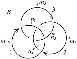 Figure 1
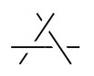 Figure 2
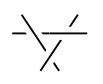 Figure 3
 Figure 4
 Figure 5
 Figure 6
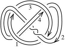 Figure 7
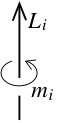 Figure 8
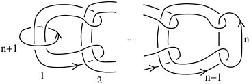 Figure 9
 Figure 10
 Figure 11
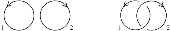 Figure 12
 Figure 13
 Figure 14
Peer Reviews
No public reviews on file for this paper yet. If you reviewed it on a platform where reviews are public (OpenReview, ICLR, NeurIPS, ICML), you can paste yours below so the community can read it here.
Videos
No videos yet. Explain this paper in a talk, walkthrough, or lecture? Add one.
Taxonomy
TopicsGeometric and Algebraic Topology · Homotopy and Cohomology in Algebraic Topology · Algebraic structures and combinatorial models
Linking number and Milnor invariants
Jean-Baptiste Meilhan
Université Grenoble Alpes, IF, 38000 Grenoble, France
Abstract.
This is a concise overview of the definitions and properties of the linking number and its higher-order generalization, Milnor invariants.
1. Introduction
The linking number is probably the oldest invariant of knot theory. In 1833, several decades before the seminal works of physicists Tait and Thompson on knot tabulation, the work of Gauss on electrodynamics led him to formulate the number of “intertwinings of two closed or endless curves” as
[TABLE]
where (resp. ) are coordinates on the first (resp. second) curve. This number, now called linking number, is an invariant of –component links,111In this note, all links will be ordered and oriented tame links in the -sphere. which typically distinguishes the trivial link and the Hopf link, shown below.
[TABLE]
Alternatively, the linking number can be simply defined in terms of the first homology group of the link complement (see Thm. 2.1). But, rather than the abelianization of the fundamental group, one can consider finer quotients, for instance by the successive terms of its lower central series, to construct more subtle link invariants. This is the basic idea upon which Milnor based his work on higher order linking numbers, now called Milnor -invariants.
We review in Section 2 several definitions and key properties of the linking number. In Section 3, we shall give a precise definition of Milnor invariants and explore some of their properties, generalizing those of the linking number. In the final Section 4, we briefly review further known results on Milnor invariants.
2. The Linking Number
The linking number has been studied from multiple angles and has thus been given many equivalent definitions of various natures. We already saw in (1) the original definition due to Gauss; let us review below a few others.
2.1. Definitions
For the rest of this section, let be a component link, and let denote the linking number of .
Recall that the first homology group of the complement of is the infinite cyclic group generated by the class of a meridian , as shown on the right.
Theorem 2.1**.**
The linking number of is the integer such that .
Recall now that any knot bounds orientable surfaces in , called Seifert surfaces. Now, given a Seifert surface for , one may assume up to isotopy that intersects at finitely many transverse points. At each intersection point, the orientation of and that of form an oriented -frame, hence a sign using the right-hand rule; the algebraic intersection of and is the sum of these signs over all intersection points.
Theorem 2.2**.**
The linking number of is the algebraic intersection of with a Seifert surface for .
Given a regular diagram of , the linking number is simply given by the number of crossings where passes over , counted with signs as follow.
Theorem 2.3**.**
[TABLE]
The proof of the above results, i.e. the fact that these definitions are all equivalent and equivalent to (1), can be found in [41, §. 5.D], along with several further definitions. See also [40] for details.
Remark 2.4*.*
As part of Theorems 2.2 and 2.3, the linking number does not depend on the choices involved in these definitions, namely the choice of a Seifert surface for and of a diagram of , respectively.
2.2. Basic properties
It is rather clear, using any of the above definitions, that reversing the orientation of either component of changes the sign of .
Also clear from Gauss formula (1) is the fact that the linking number is symmetric :
[TABLE]
This can also be seen, for example, from the diagrammatic definition (Thm. 2.3), by considering two projections, on two parallel planes which are ‘on either sides’ of , so that crossings where overpasses in one diagram are in one-to-one correspondence with crossings where overpasses in the other, with same sign.
The symmetry property (2) allows for a symmetrized version of Theorem 2.3:
[TABLE]
where the sum runs over all crossings involving a strand of component and a strand of component .
2.3. Two classification results
The following notion was introduced by Milnor in the fifties [29].
Definition 2.5**.**
Two links are link-homotopic if they are related by a sequence of ambient isotopies and self-crossing changes, i.e. crossing changes involving two strands of a same component (see Figure 1).
The idea behind this notion is that, as a first approximation to the general study of links, working up to link-homotopy allows to unknot each individual component of a link, and only records their ‘mutual interractions’ – this is in a sense studying ‘linking modulo knotting’.
Observe that the linking number is invariant under link-homotopy. Furthermore, it is not too difficult to check that any –component link is link-homotopic to an iterrated Hopf link, i.e. the closure of the pure braid for some . This number is precisely the linking number of the original link, thus showing:
Theorem 2.6**.**
The linking number classifies -component links up to link-homotopy.
Generalizing this result to a higher number of components, however, requires additional invariants, and this was one of the driving motivations that led Milnor to develop his -invariants, see Section 3.3.2.
The equivalence relation on links with an arbitrary number of components which is classified by the linking number is the -equivalence, which is generated by the -move, shown on the right-hand side of Figure 1. Indeed, the following is due H. Murakami and Y. Nakanishi [32], see also [26].
Theorem 2.7**.**
Two links and () are -equivalent if, and only if for all such that .
Notice in particular that the -move is an unknotting operation, meaning that any knot can be made trivial by a finite sequence of isotopies and -moves.
3. Milnor invariants
In this whole section, let be an -component link, for some fixed .
3.1. Definition of Milnor -invariants
In his master’s and doctoral theses, supervised by R. Fox, Milnor defined numerical invariants extracted from the peripheral system of a link, which widely generalize the linking number.
Denote by the complement of an open tubular neighborhood of . Pick a point in the interior of , and denote by the fundamental group of based at this point. It is well-known that, given a diagram of , we can write an explicit presentation of , called Wirtinger presentation, where each arc in the diagram provides a generator, and each crossing yields a relation. Such presentations, however, are in general difficult to work with, owing to their large number of generators. We introduce below a family of quotients of for which a much simpler presentation can be given, and which still retain rich topological information on the link .
The lower central series of a group is the nested family of subgroups defined inductively by
[TABLE]
The th nilpotent quotient of the group is the quotient .
Let us fix, from now on, a value of . For each , consider two elements , where represents a choice of a meridian for in , and where is a word representing the th preferred longitude of , i.e. a parallel copy of in having linking number zero with . Denote also by the free group .
Theorem 3.1** (Chen-Milnor Theorem).**
The th nilpotent quotient of has a presentation given by
[TABLE]
In order to extract numerical invariants from the nilpotent quotients of , we consider the Magnus expansion [25] of each , which is an element of , the ring of formal power series in non commuting variables , obtained by the substitution
[TABLE]
We denote by the coefficient of in the Magnus expansion of :
[TABLE]
This coefficient is not, in general, an invariant of the link, as it depends upon the choices made in this construction (Essentially, picking a system of based meridians for ). We can, however, promote these number to genuine invariants by regarding them modulo the following indeterminacy.
Definition 3.2**.**
Given a sequence of indices in , let be the greatest common divisor of the coefficients , for all sequences obtained from by deleting at least one index and permuting cyclicly.
For example, .
Theorem–Definition** (Milnor [30]).**
The residue class
[TABLE]
is an invariant of ambient isotopy of , for any sequence of integers, called a Milnor invariant of . The number of indices in is called the length.
Before giving some examples, in Section 3.2, a few remarks are in order.
Remark 3.3*.*
Observe from (3) that is only defined for a sequence of two or more indices. We set for all as a convention.
Remark 3.4*.*
If all Milnor invariants of of length are zero, then those of length are well defined integers. These first non-vanishing Milnor invariants are thus much easier to study in practice and, as a matter of fact, a large proportion of the literature on Milnor link invariants focusses on them.
Remark 3.5*.*
Working with the th nilpotent quotient of only allows to define Milnor invariants up to length . But this can be chosen arbitrarily large, so this is no restriction.
3.2. First examples
By Remark 3.3, length Milnor invariants are well-defined over . In order to define them, it suffices to work in the second nilpotent quotient, i.e. in . But the th preferred longitude in is given by , and we have
[TABLE]
Hence length Milnor invariants are exactly the pairwise linking numbers of a link. This justifies regarding length Milnor invariants as ‘higher order linking numbers’. In order to get a grasp on these, let us consider an elementary example.
Example 3.6*.*
Consider the Boromean rings , as illustrated below.222 There, we use the usual convention that a small arrow underpassing an arc of the diagram represents a loop, based at the reader’s eye and going straight down to the projection plane, enlacing positively the arc and going straight back to the basepoint. The Wirtinger presentation for is
\quad\pi=\left\langle\begin{array}[]{c|ccc}m_{1}\,,\,m_{2}\,,\,m_{3}&m_{3}m_{1}m_{3}^{-1}n_{1}^{-1}\,\,;&m_{1}m_{2}m_{1}^{-1}n_{2}^{-1}\,\,;&m_{2}m_{3}m_{2}^{-1}n_{3}^{-1}\\ n_{1}\,,\,n_{2}\,,\,n_{3}&n_{1}^{-1}n_{2}n_{1}m_{2}^{-1}\,\,;&n_{2}^{-1}n_{3}n_{2}m_{3}^{-1}\,\,;&n_{3}^{-1}n_{1}n_{3}m_{1}^{-1}\end{array}\right\rangle.\qquad\qquad\qquad
Consider the third nilpotent quotient of , i.e. fix . We choose the meridians as (representatives of) generators, and express preferred longitudes : we have (the other two are obtained by cyclic permutation of the indices, owing to the symmetry of the link). Taking the Magnus expansion gives
[TABLE]
We thus obtain that for any sequences of two indices (i.e. all linking numbers are zero), and
[TABLE]
Example 3.6 illustrates the fact that, just like the linking number detects (and actually, counts copies of) the Hopf link, the triple linking number detects the Borromean rings. This generalizes to the following realization result, due to Milnor [29].
Lemma 3.7**.**
*Let be the -component link shown on the right
(), and let be any permutation in . Then*
\quad\overline{\mu}_{M_{n}}\left(\sigma(1)\cdots\sigma(n-1)n(n+1)\right)=\left\{\begin{array}[]{cc}1&\textrm{if \sigma=Id,}\\ 0&\textrm{otherwise.}\end{array}\right.**
[TABLE]
3.3. Some properties
We gather here several well-known properties of Milnor -invariants, most being due to Milnor himself [29, 30] (unless otherwise specified).
3.3.1. Symmetry and Shuffle
It is rather clear that, if is obtained from by reversing the orientation of the th component, then , where denotes the number of occurences of the index in the sequence . The next two relations were shown by Milnor [30], using properties of the Magnus expansion:
**Cyclic symmetry: ** For any sequence of indices in , we have
[TABLE]
**Shuffle: ** For any and any two sequences of indices in , we have
[TABLE]
where denotes the set of all sequences obtained by inserting the indices of into , preserving order.
It follows in particular that there is essentially only one triple linking number: for any -component algebraically split link , we have
In general, the number of independent -invariants was given by K. Orr, see [36, Thm. 15].
3.3.2. Link-homotopy and concordance
Milnor invariants are not only invariants of ambiant isotopy: they are actually invariants of isotopy, i.e. homotopy through embeddings. In particular that Milnor invariants do not see ’local knots’.
As mentioned in Section 2.3, the notion of link-homotopy was introduced by Milnor himself, who proved the following in [30].
Theorem 3.8**.**
For any sequence of pairwise distinct indices, is a link-homotopy invariant.
Milnor invariants are sharp enough to detect link-homotopically trivial links, and to classify links up to link-homotopy for components [30]. The case of -component links was only completed thirty years later by J. Levine, using a refinement of Milnor’s construction [20]. The general case is discussed in Section 4.1. Milnor link-homotopy invariants also form a complete set of link-homotopy invariants for Brunnian links, i.e. links which become trivial after removal of any component (see Section 3.2 for examples) [29].
Recall that two -component links and are concordant if there is an embedding of disjoint copies of the annulus , such that and . The following was essentially shown by J. Stallings [43] (and also by A. Casson [6] for the more general relation of cobordism).
Theorem 3.9**.**
Milnor invariants are concordance invariants.
Let us also mention here that Milnor invariants are all zero for a boundary link, that is, for a link whose components bound mutually disjoint Seifert surfaces in [42]. Characterizing geometrically links with vanishing of Milnor invariants is the subject of the -slice conjecture, proved by K. Igusa and K. Orr in [14], which roughly states that all invariants of length vanish if and only if the link bounds a surface which “looks like slice disks” modulo -fold commutators of the fundamental group of the surface complement.
3.3.3. Cabling formula
Milnor invariants indexed by non-repeated sequences are not only topologically relevant, by Theorem 3.8; they also ‘generate’ all Milnor invariants, by the following.
Theorem 3.10**.**
Let be a sequence of indices in , such that the index appears twice in . Then , where is obtained from by replacing the second occurence of by , and where is obtained from by adding an th component, which is a parallel copy of having linking number zero with it.
Example 3.11*.*
A typical example of a link-homotopically trivial link is the Whitehead link , shown below
[TABLE]
on the left-hand side. But Milnor concordance invariants do detect ; specifically, we have .
As a matter of fact, one can check that
[TABLE]
where is the -component link shown on the right.
[TABLE]
3.3.4. Additivity
Given two -component links and , lying in two disjoint -balls of , a band sum of an is any link made of pairwise disjoint connected sums of the th components of and (). Although this operation is not well-defined, V. Krushkal showed that, for any sequence ,
[TABLE]
meaning that Milnor invariants are independent of the choice of bands defining , see [19].
4. Further properties
Since their introduction in the fifties, Milnor invariants have been the subject of numerous works. In this section, which claims neither exhaustivity nor precision, we briefly overview some of these results.
4.1. Refinements and generalizations
The main difficulty in understanding Milnor -invariants lies in these intricate indeterminacies . Multiple attempts have been made to refine this indeterminacy, in order to get more subtle invariants.
T. Cochran defined, by considering recursive intersection curves of Seifert surfaces, link invariants which recover (and shed beautiful geometric lights on) -invariants, and sometimes refine them [8].
K. Orr defined invariants, as the class of the ambient in some third homotopy group, which refines significantly the indeterminacy of Milnor invariants [35, 36]. Orr’s invariant is also the first attempt towards a transfinite version of Milnor invariants, a problem posed in [30]; see also the work of J. Levine in [22].
A decisive step was taken by Habegger and Lin, who showed that the indeterminacies are equivalent to the indeterminacy in representing as the closure of a string link, i.e. a pure tangle without closed component [11] (see also [21]). This led them to a full link-homotopy classification of (string) links [11].
4.2. Link maps and higher dimensional links
There are several higher dimensional versions of the linking number; see [5, § 3.4] for a good survey. Some are invariants of link maps, i.e. maps from a union of two spheres (of various dimensions) to a sphere with disjoint images – these are the natural objects to consider when working up to link-homotopy. In particular, the first example of a link map which is not link-homotopically trivial was given in [9] using an appropriate generalization of the linking number.
Higher dimensional generalizations of Milnor invariants were defined and extensively studied by U. Koschorke for link maps with many components, see [16, 17] and references therein. Note also that Orr’s invariants, which generalize Milnor invariants (see Section 4.1), are also defined in any dimensions. But there does not seem to be nontrivial analogues of Milnor invariants for -dimensional links (), i.e. for embedded -spheres in codimension ; in fact, all are link-homotopically trivial [4]. However, Milnor invariants generalize naturally to -string links, i.e. knotted annuli in the -ball bounded by a prescribed unlink in the -sphere, and classify them up to link-homotopy [2], thus providing a higher dimensional version of [11].
4.3. Relations with other invariants
Milnor invariants are not only natural generalizations of the linking number, but are also directly related to this invariant. Indeed, K. Murasugi expressed Milnor -invariants of a link as a linking number in certain branched coverings of along this link [34]. The Alexander polynomial is also rather close in nature to Milnor invariants, being extracted from the fundamental group of the complement. As a matter of fact, there are a number of results relating these two invariants: see for example [7, 23, 33, 37, 44]. On the other hand, the relation to the Konstevich integral [12] hints to potential connections to quantum invariants. Such relations were given with the HOMFLY-PT polynomial [28] and the (colored) Jones polynomial [27]. Milnor string link invariants also satisfy a skein relation [38], which is a typical feature of polynomial and quantum invariants.
There also are known relations outside knot theory. Milnor -invariants can be expressed in terms of Massey products of the complement, which are higher order cohomological invariants generalizing the cup product [39, 45]. Also, Milnor string link invariants are in natural correspondence with Johnson homomorphisms of homology cylinders, which are -dimensional extensions of certain abelian quotients of the mapping class group [10]. Finaly, as part of the deep analogies he established between knots and primes, M. Morishita defined and studied arithmetic analogues of Milnor invariants for prime numbers [31].
4.4. Finite type invariants
The linking number is (up to scalar) the unique degree finite type link invariant. This was generalized independently by D. Bar Natan [3] and X.S. Lin [24], who showed that any Milnor string link invariant of length is a finite type invariant of degree . As a consequence, Milnor string link invariants can be, at least in principle, extracted from the Kontsevich integral, which is universal among finite type invariants. This was made completely explicit by G. Masbaum and N. Habegger in [12].
Note that the finite type property does not make sense for higher order -invariants (of links), since the indeterminacy is in general not the same for two links which differ by a crossing change. Nonetheless, -invariants of length are invariants of -equivalence [13], a property shared by all degree invariants.
4.5. Virtual theory
There are two distinct extensions of the linking number for virtual -component links, namely and , where is the sum of signs of crossings where passes over . Notice that these virtual linking numbers are actually invariants of welded links, i.e. are invariant under the forbidden move allowing a strand to pass over a virtual crossing. Indeed, the linking number is extracted from (a quotient of) the fundamental group, which is a welded invariant [15]. Likewise, extensions of Milnor invariants shall be welded invariants. A general welded extension of Milnor string link invariants is given in [1], which classifies welded string links up to self-virtualization, generalizing the classification of [11]. This extension recovers and extends that of [18], which gives general Gauss diagram formulas for virtual Milnor invariants.
Acknowledgments*.*
The author would like to thank Benjamin Audoux and Akira Yasuhara, for their comments on a preliminary version of this note.
The reference list from the paper itself. Each links out to its DOI / PubMed record.
- 1[1] B. Audoux, P. Bellingeri, J.-B. Meilhan, and E. Wagner. Homotopy classification of ribbon tubes and welded string links. Ann. Sc. Norm. Super. Pisa Cl. Sci. , XVII(2):713–761, 2017.
- 2[2] B. Audoux, J.-B. Meilhan, and E. Wagner. On codimension 2 2 2 embeddings up to link-homotopy. J. Topology , 10(4):1107–1123, 2017.
- 3[3] D. Bar-Natan. Vassiliev homotopy string link invariants. J. Knot Theory Ramifications , 4(1):13–32, 1995.
- 4[4] A. Bartels and P. Teichner. All two dimensional links are null homotopic. Geom. Topol. , 3:235–252, 1999.
- 5[5] J. Carter, S. Kamada, and M. Saito. Surfaces in 4-space , volume 142 of Encyclopaedia of Mathematical Sciences . Springer-Verlag, Berlin, 2004. Low-Dimensional Topology, III.
- 6[6] A. Casson. Link cobordism and Milnor’s invariant. Bull. Lond. Math. Soc. , 7:39–40, 1975.
- 7[7] T. D. Cochran. Concordance invariance of coefficients of Conway’s link polynomial. Invent. Math. , 82(3):527–541, 1985.
- 8[8] T. D. Cochran. Derivatives of links: Milnor’s concordance invariants and Massey’s products. Mem. Am. Math. Soc. , 427:73, 1990.