Implications of nuclear interaction for nuclear structure and astrophysics within the relativistic mean-field model
Bharat Kumar

TL;DR
This paper explores how nuclear interactions influence nuclear structure and astrophysical phenomena using the relativistic mean-field model, providing insights into the fundamental forces shaping atomic nuclei and stellar objects.
Contribution
It applies the relativistic mean-field model to analyze nuclear interactions and their implications for nuclear structure and astrophysics, offering new theoretical insights.
Findings
Enhanced understanding of nuclear forces within RMF model
Implications for neutron star properties and nuclear stability
Potential predictions for exotic nuclei
Abstract
In this dissertation, we have studied the implications of nuclear interaction for nuclear structure and astrophysics within the relativistic mean-field (RMF) model.
Click any figure to enlarge with its caption.
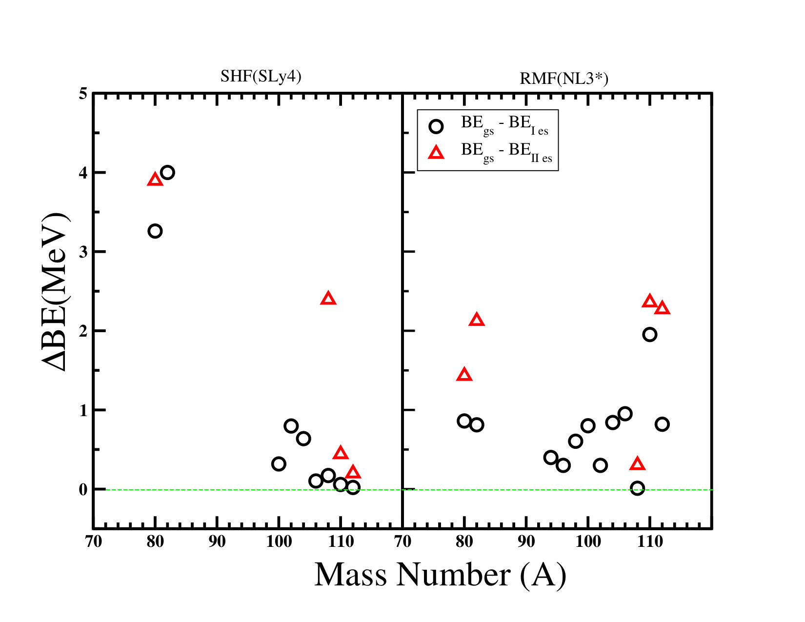 Figure 1
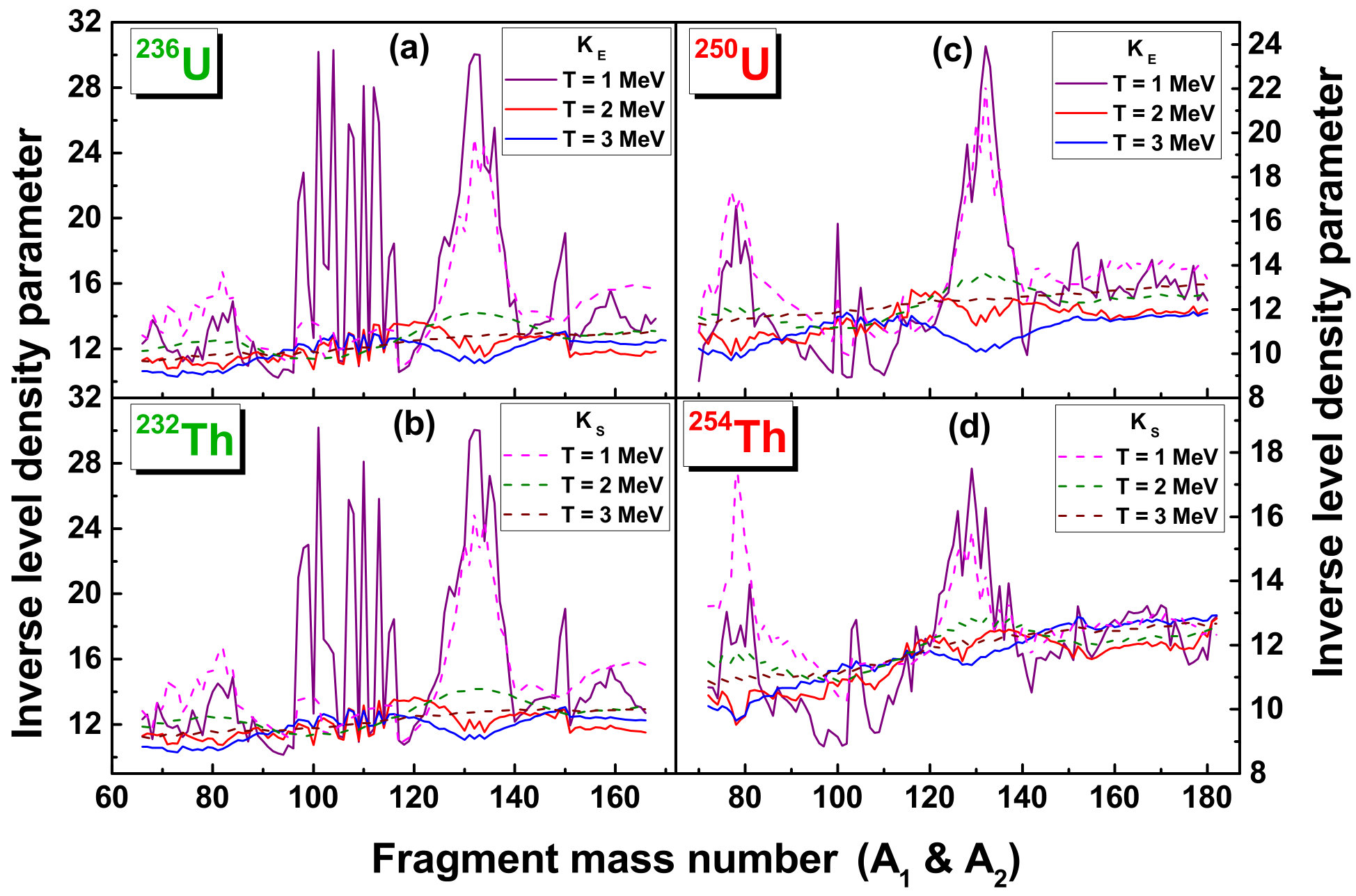 Figure 4
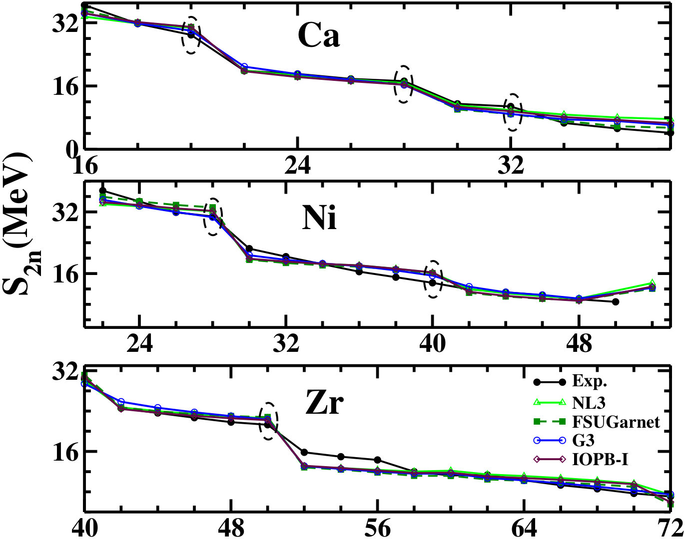 Figure 5
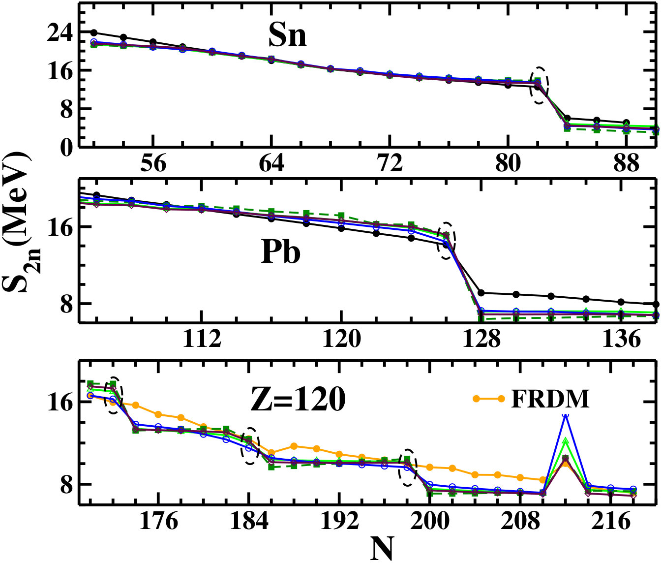 Figure 6
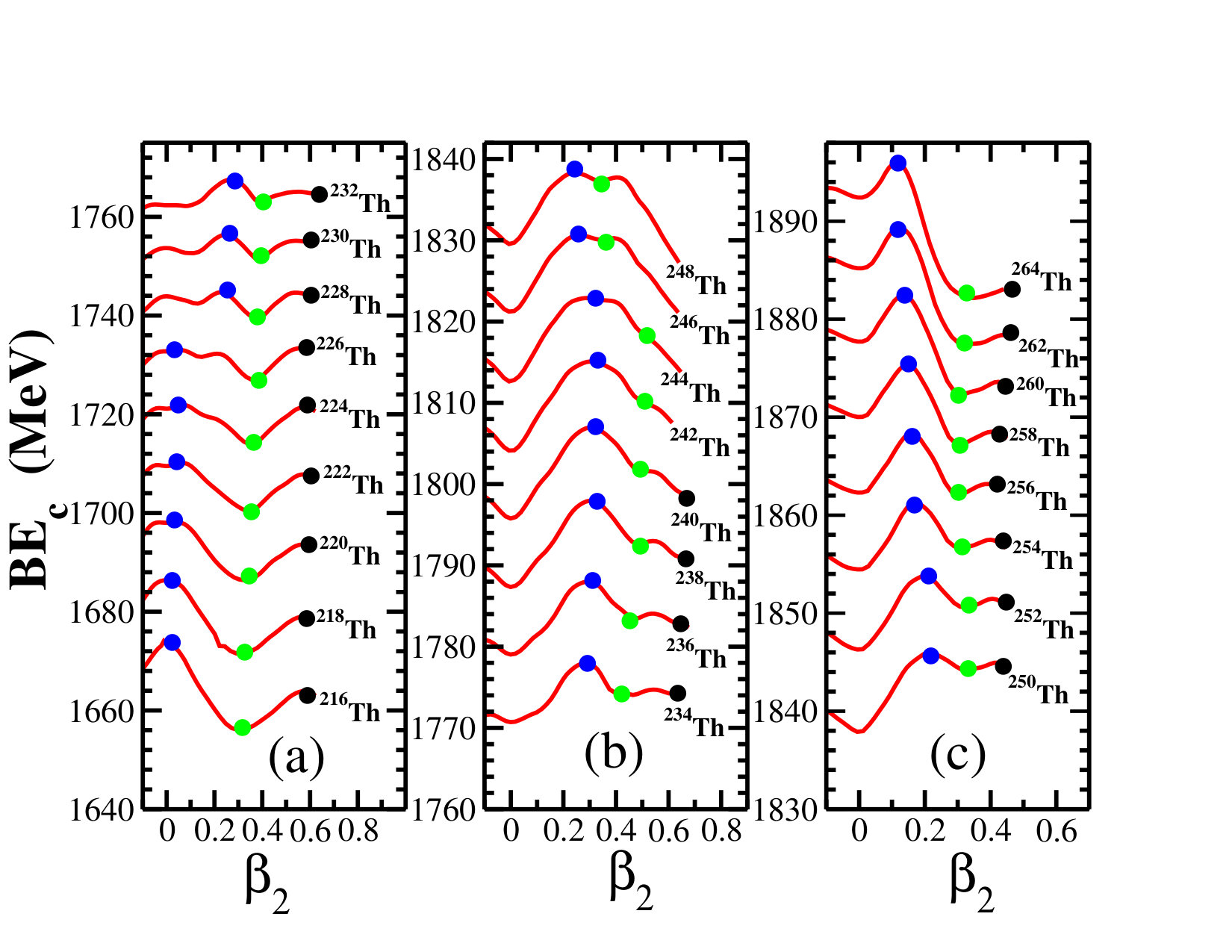 Figure 7
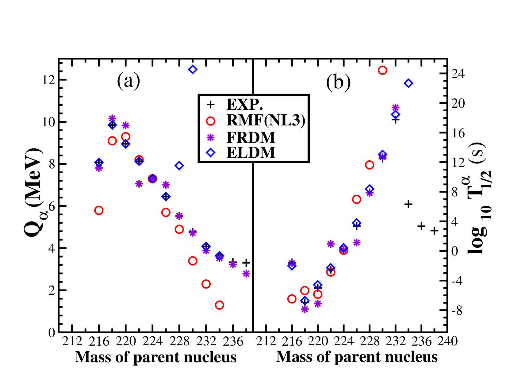 Figure 8
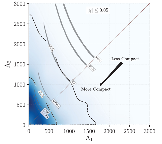 Figure 9
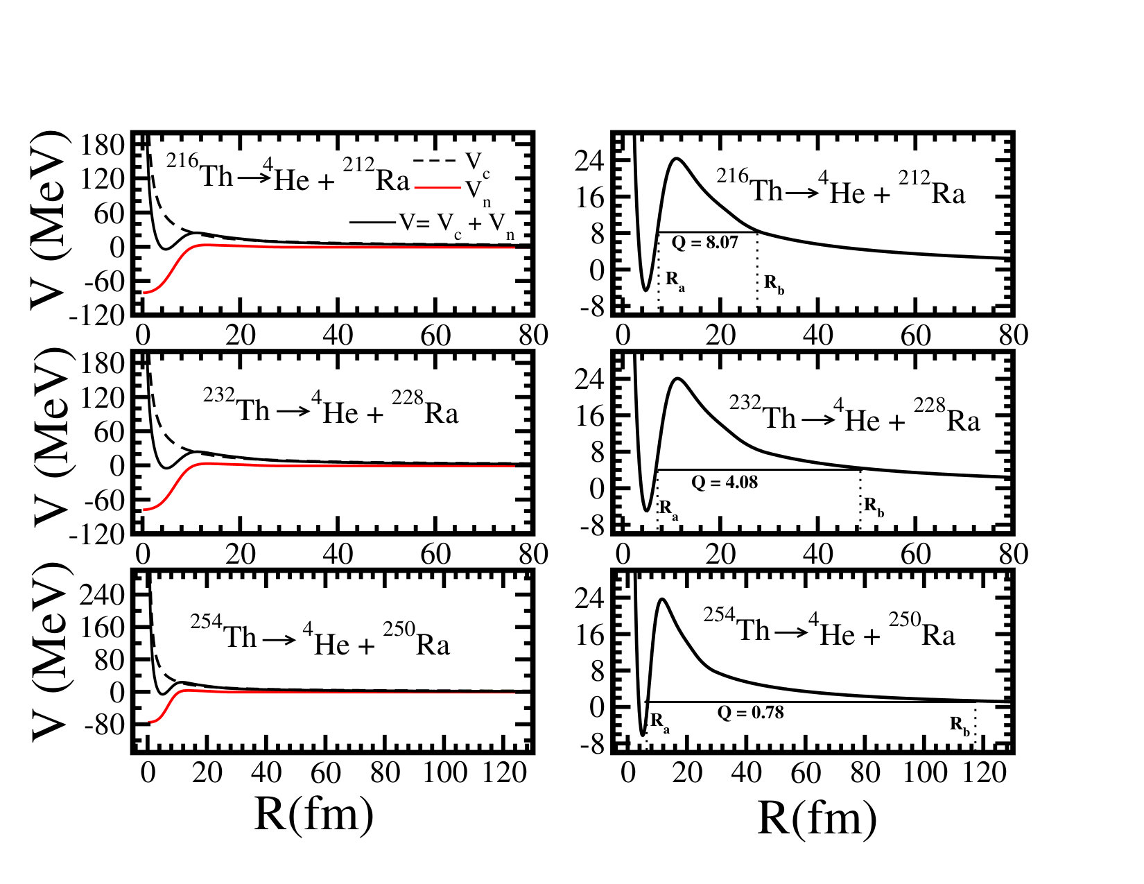 Figure 10
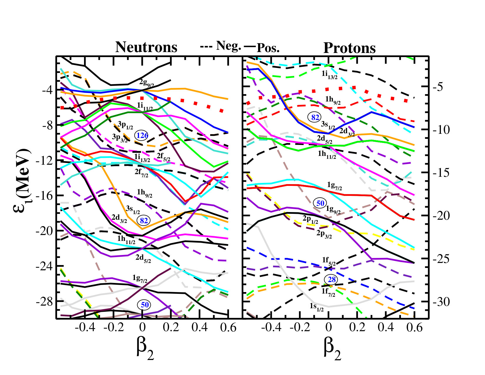 Figure 11
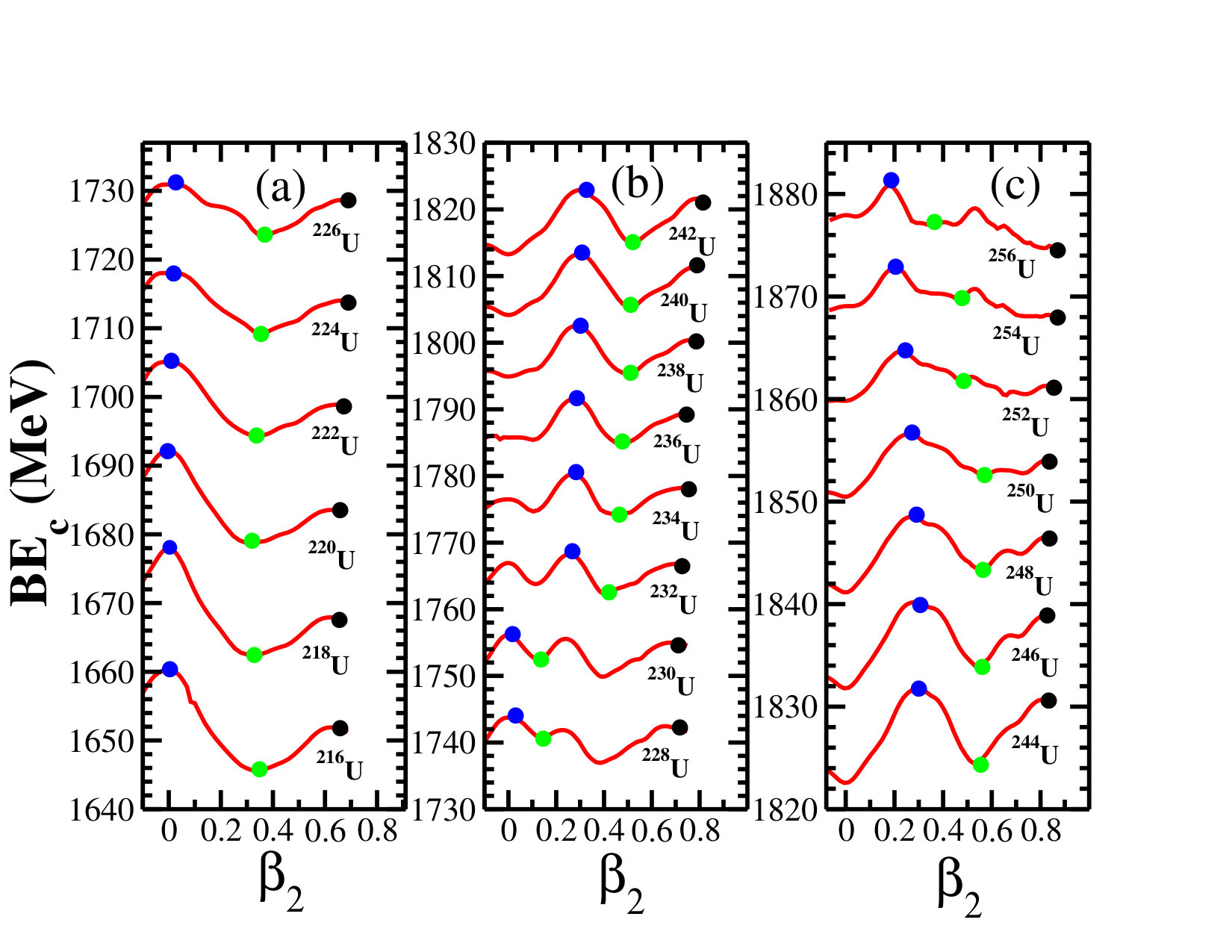 Figure 12
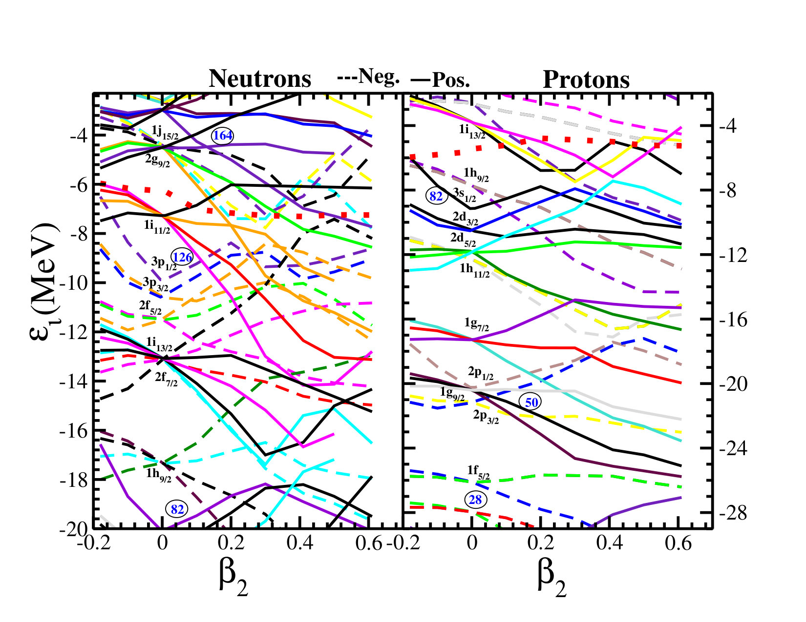 Figure 13
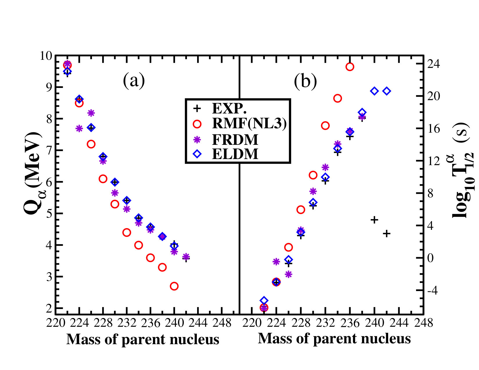 Figure 14
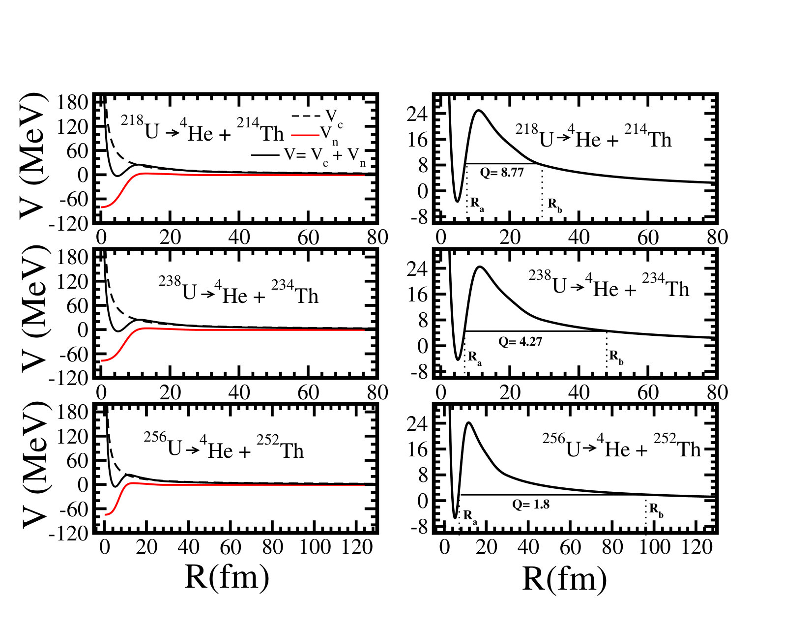 Figure 15
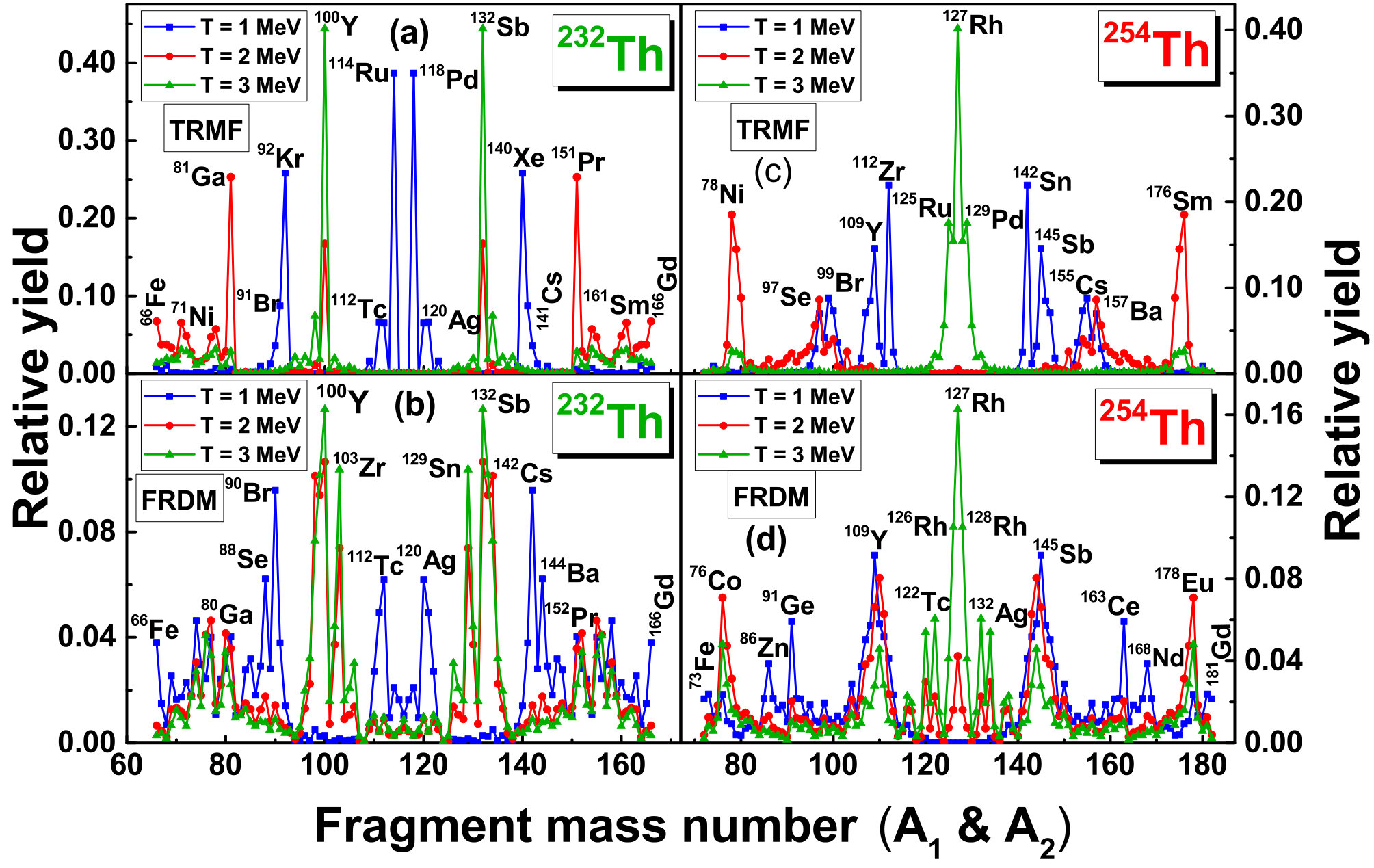 Figure 16
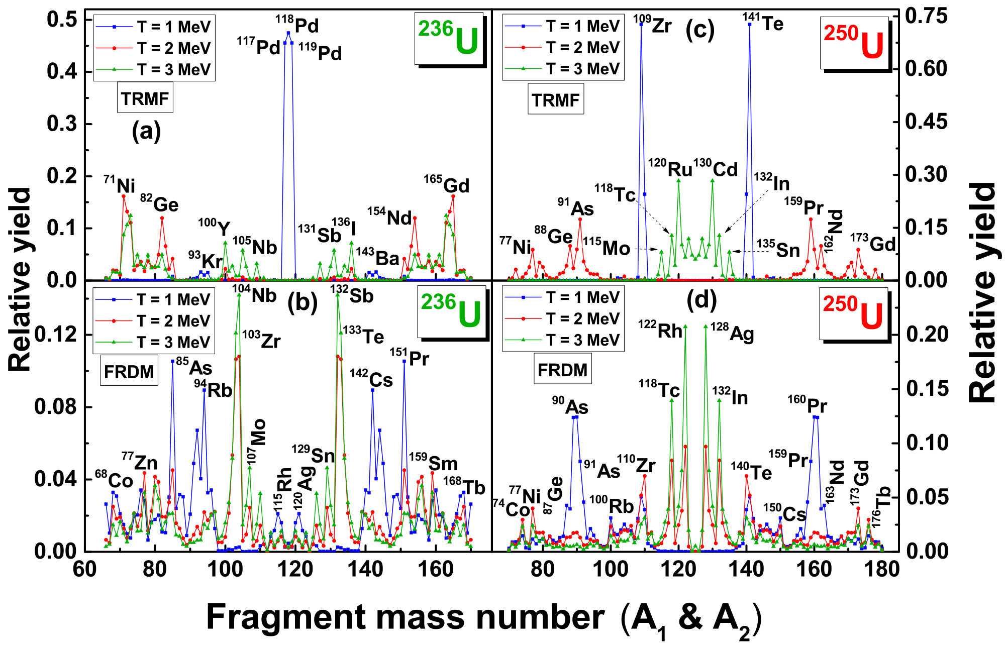 Figure 17
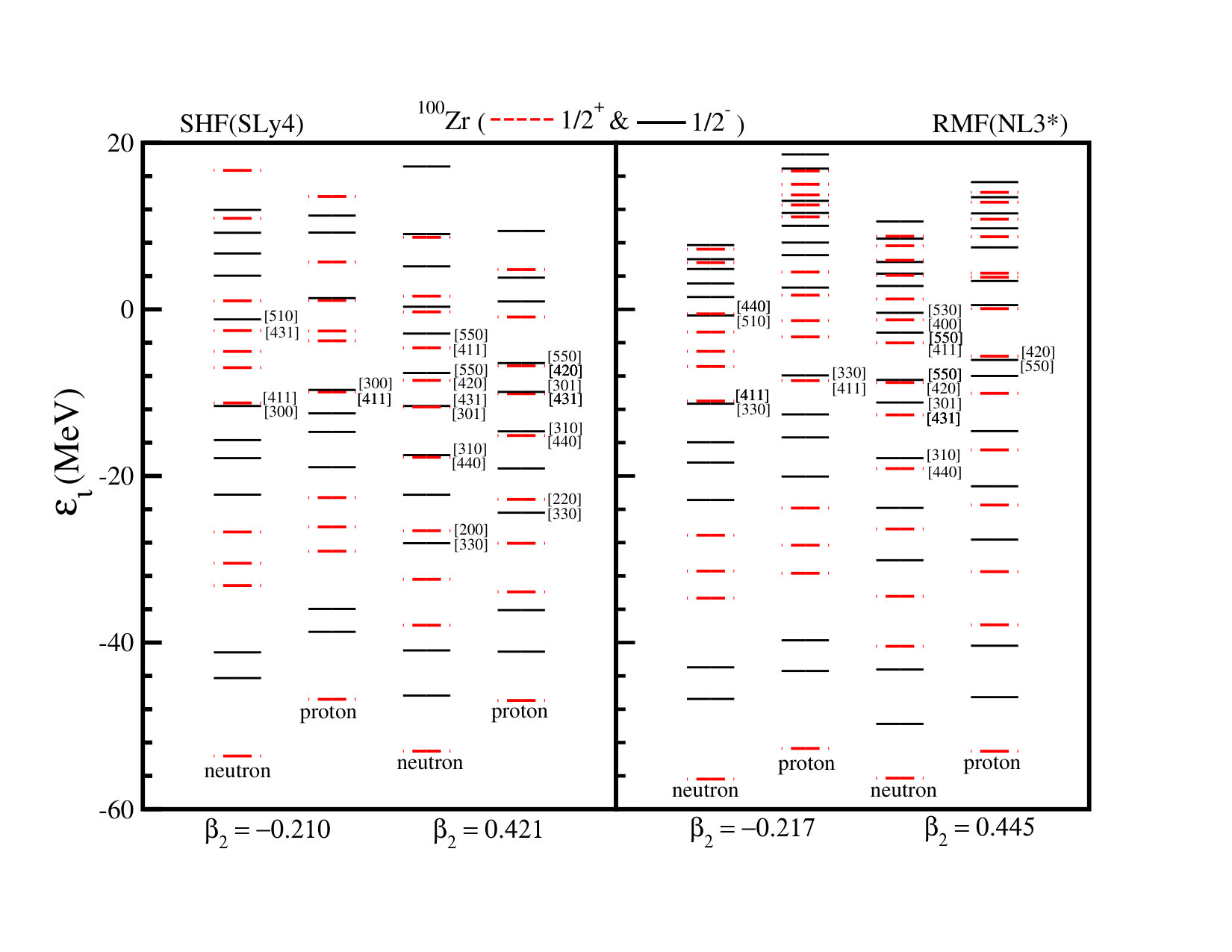 Figure 18
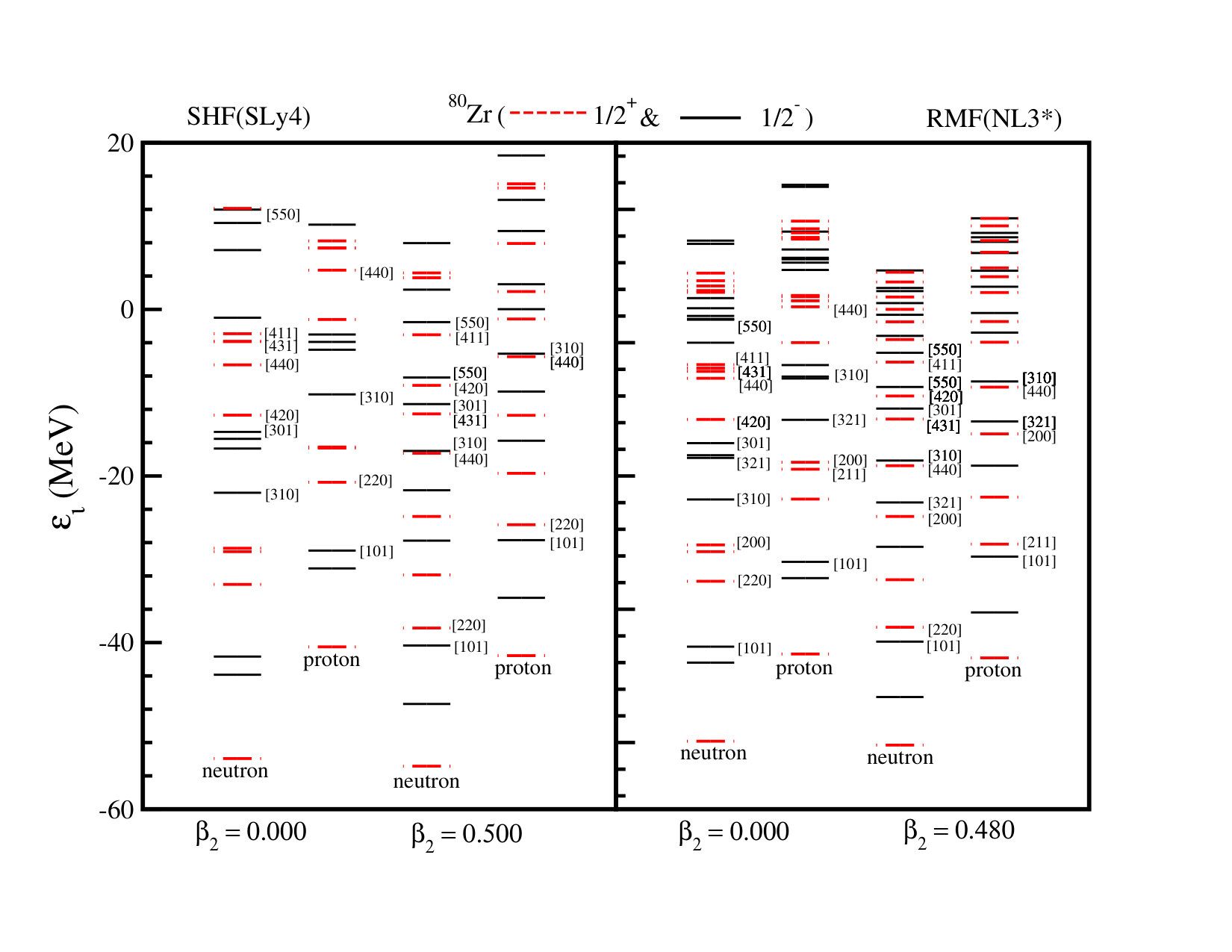 Figure 19
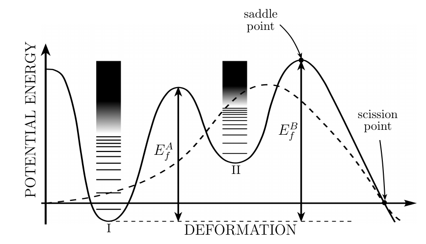 Figure 20
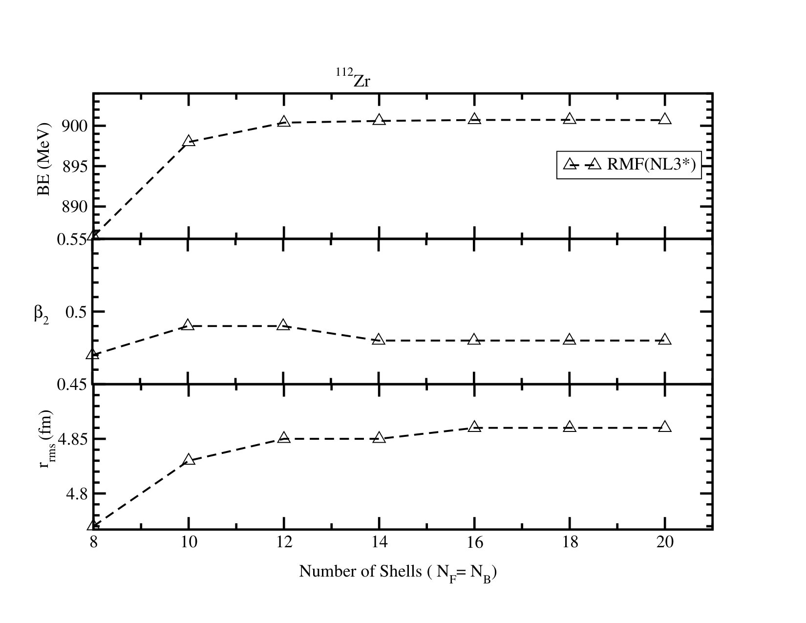 Figure 21
 Figure 22
 Figure 23
 Figure 24
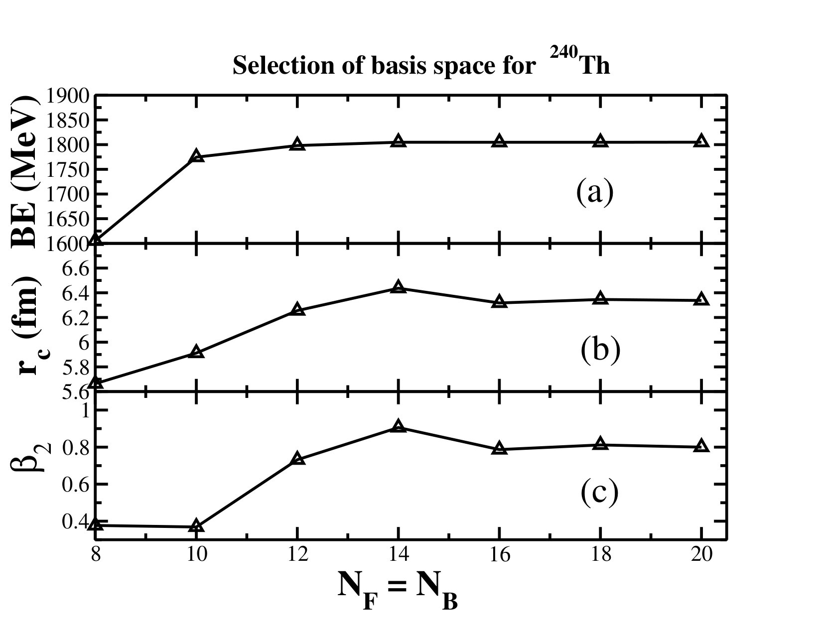 Figure 25
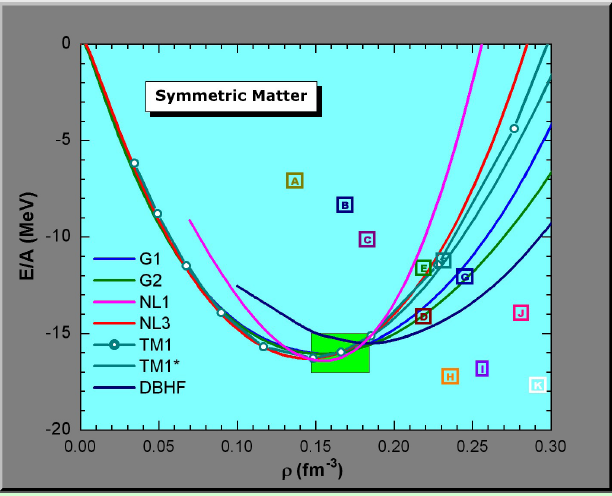 Figure 26
 Figure 27
 Figure 28
 Figure 29
 Figure 30
 Figure 31
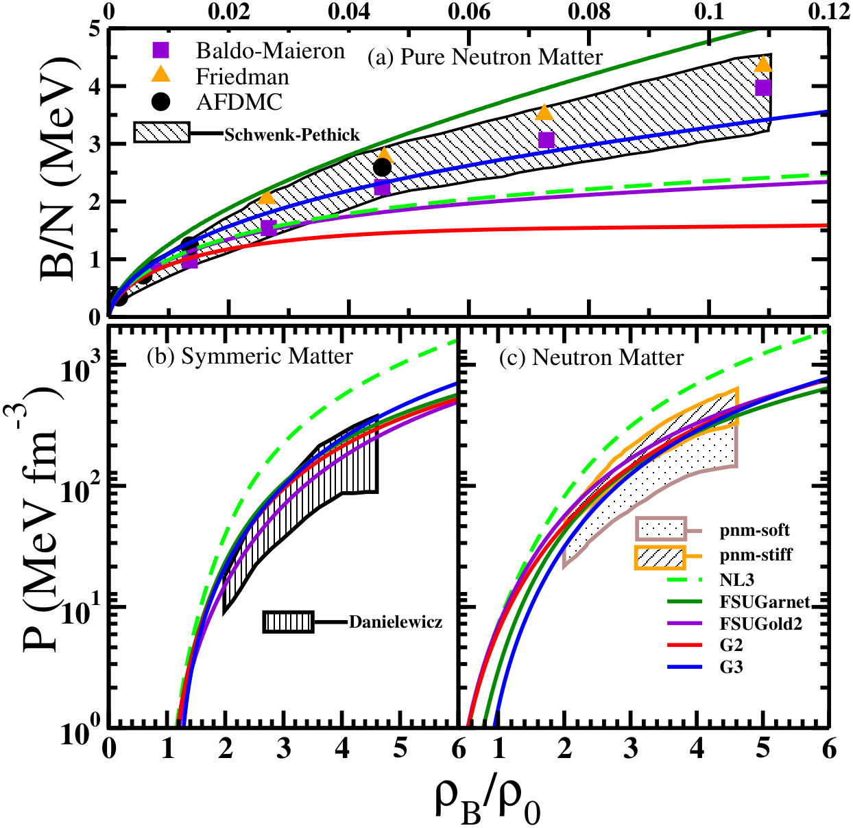 Figure 32
 Figure 33
 Figure 1
 Figure 35
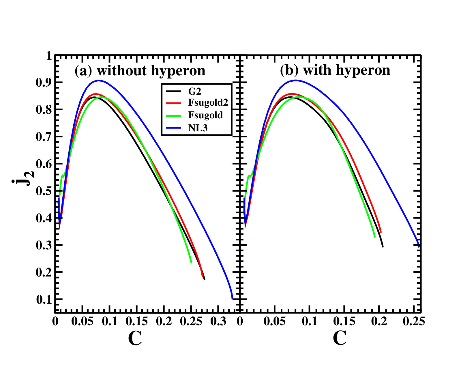 Figure 36
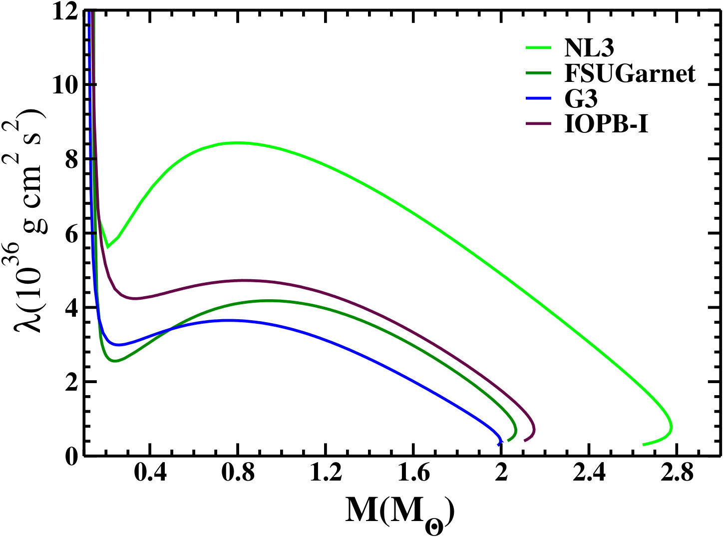 Figure 37
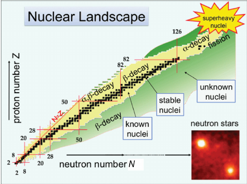 Figure 38
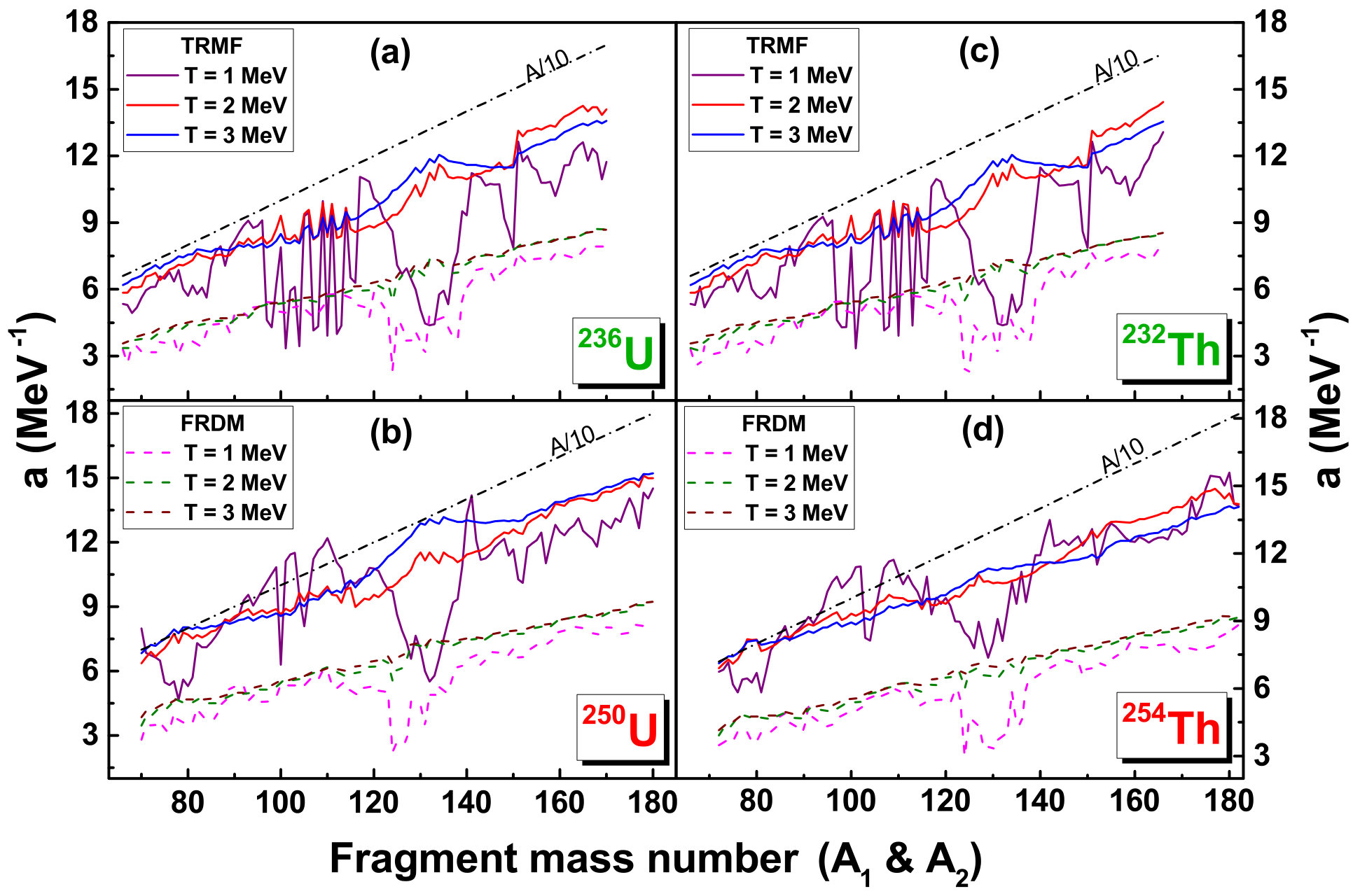 Figure 39
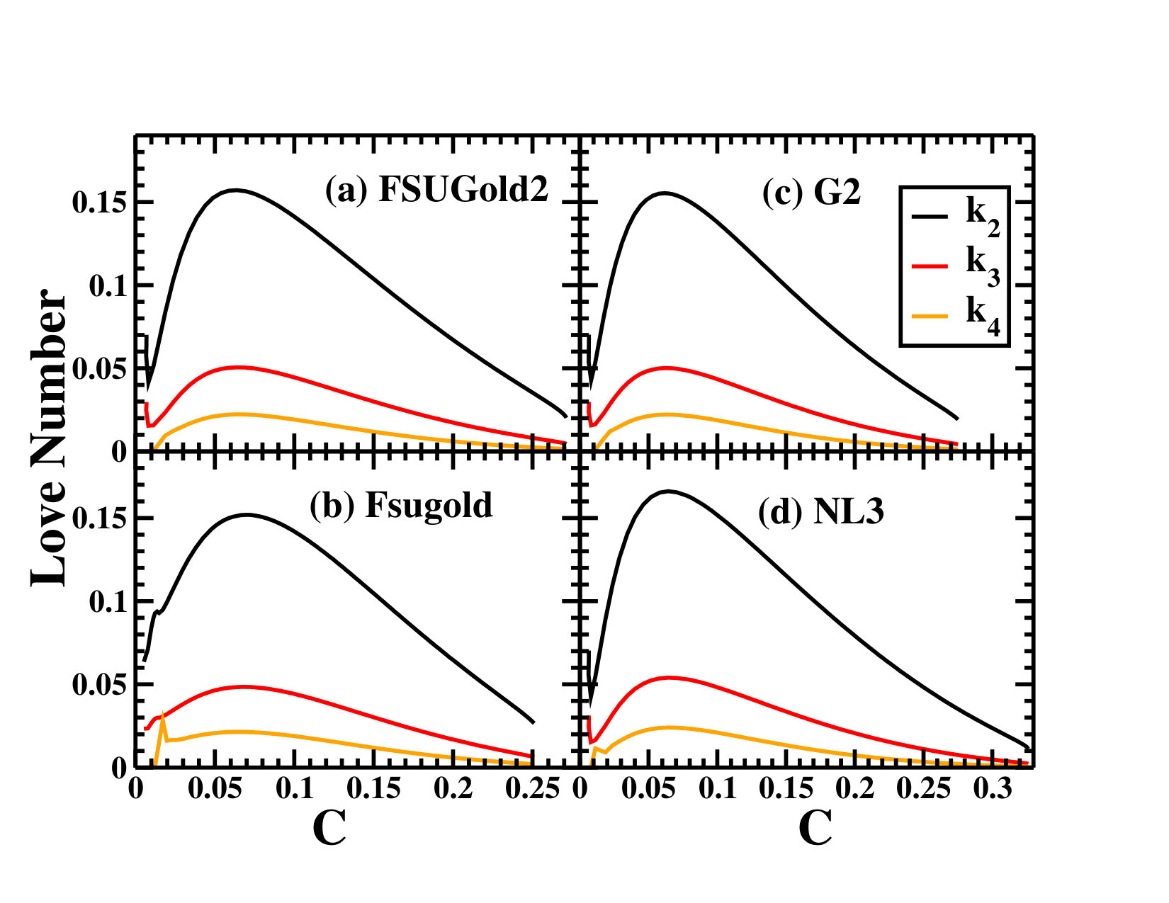 Figure 40
| RMF (NL3) | FRDM | Experiment | |||||||||
| Nucleus | BE (MeV) | BE(MeV) | BE (MeV) | ||||||||
| 216U | 5.762 | 5.616 | 5.700 | 5.673 | 0 | 1660.5 | 1649.0 | -0.052 | |||
| 6.054 | 5.946 | 6.008 | 5.999 | 0.608 | 1650.8 | ||||||
| 218U | 5.789 | 5.625 | 5.721 | 5.682 | 0 | 1678.0 | 1666.7 | 0.008 | 1665.6 | ||
| 6.081 | 5.957 | 6.029 | 6.011 | 0.606 | 1666.9 | ||||||
| 220U | 5.819 | 5.641 | 5.745 | 5.698 | 0 | 1692.2 | 1681.2 | 0.008 | 1680.8 | ||
| 6.109 | 5.971 | 6.052 | 6.025 | 0.605 | 1682.6 | ||||||
| 222U | 5.849 | 5.661 | 5.772 | 5.717 | 0 | 1705.1 | 1695.7 | 0.048 | 1695.6 | ||
| 6.142 | 5.990 | 6.079 | 6.043 | 0.611 | 1697.9 | ||||||
| 224U | 5.878 | 5.681 | 5.798 | 5.737 | 0 | 1717.9 | 1710.8 | 0.146 | 1710.3 | ||
| 6.198 | 6.032 | 6.131 | 6.085 | 0.645 | 1712.8 | ||||||
| 226U | 5.907 | 5.701 | 5.824 | 5.757 | 0 | 1730.8 | 1724.7 | 0.172 | 1724.8 | ||
| 6.232 | 6.053 | 6.160 | 6.106 | 0.652 | 1727.4 | ||||||
| 5.935 | 5.721 | 5.850 | 5.776 | 0 | 1743.6 | ||||||
| 228U | 5.966 | 5.743 | 5.877 | 5.798 | 0.210 | 1741.7 | 1739.0 | 0.191 | 1739 | ||
| 6.259 | 6.068 | 6.182 | 6.120 | 0.651 | 1741.3 | ||||||
| 230U | 5.964 | 5.739 | 5.875 | 5.795 | 0 | 1756.0 | 1752.6 | 0.199 | 0.260 | 1752.8 | |
| 6.000 | 5.765 | 5.907 | 5.821 | 0.234 | 1755.4 | ||||||
| 6.293 | 6.091 | 6.213 | 6.143 | 0.658 | 1753.7 | ||||||
| 232U | 5.994 | 5.755 | 5.900 | 5.810 | 0 | 1766.8 | 1765.7 | 0.207 | 0.267 | 1765.9 | |
| 6.033 | 5.785 | 5.935 | 5.840 | 0.251 | 1768.2 | ||||||
| 6.364 | 6.167 | 6.286 | 6.218 | 0.712 | 1766.8 | ||||||
| 234U | 6.021 | 5.767 | 5.923 | 5.823 | 0 | 1776.4 | 1778.2 | 0.215 | 5.829 | 0.265 | 1778.6 |
| 6.065 | 5.803 | 5.963 | 5.858 | 0.267 | 1780.3 | ||||||
| 6.415 | 6.209 | 6.334 | 6.260 | 0.738 | 1778.2 | ||||||
| 236U | 6.092 | 5.819 | 5.987 | 5.874 | 0.276 | 1791.7 | 1790.0 | 0.215 | 5.843 | 0.272 | 1790.4 |
| 6.446 | 6.230 | 6.363 | 6.281 | 0.744 | 1789.4 | ||||||
| 238U | 6.124 | 5.838 | 6.015 | 5.892 | 0.283 | 1802.5 | 1801.2 | 0.215 | 5.857 | 0.272 | 1801.7 |
| 6.488 | 6.263 | 6.402 | 6.314 | 0.763 | 1800.4 | ||||||
| RMF (NL3) | FRDM | Experiment | |||||||||
| Nucleus | BE (MeV) | BE (MeV) | BE(MeV) | ||||||||
| 216Th | 5.781 | 5.594 | 5.704 | 5.651 | 0 | 1673.5 | 1663.6 | 0.008 | 1662.7 | ||
| 6.034 | 5.897 | 5.977 | 5.951 | 0.567 | 1663.8 | ||||||
| 218Th | 5.812 | 5.611 | 5.730 | 5.667 | 0 | 1686.5 | 1677.2 | 0.008 | 1676.7 | ||
| 6.105 | 5.959 | 6.045 | 6.013 | 0.616 | 1678.2 | ||||||
| 220Th | 5.842 | 5.631 | 5.757 | 5.687 | 0 | 1698.1 | 1690.2 | 0.030 | 1690.6 | ||
| 6.140 | 5.983 | 6.076 | 6.036 | 0.624 | 1692.8 | ||||||
| 222Th | 5.873 | 5.651 | 5.784 | 5.707 | 0 | 1709.7 | 1704.6 | 0.111 | 0.151 | 1704.2 | |
| 6.174 | 6.007 | 6.107 | 6.060 | 0.631 | 1706.1 | ||||||
| 224Th | 5.902 | 5.672 | 5.81 | 5.728 | 0 | 1721.4 | 1717.4 | 0.164 | 0.173 | 1717.6 | |
| 6.222 | 6.021 | 6.142 | 6.074 | 0.640 | 1718.9 | ||||||
| 226Th | 5.931 | 5.692 | 5.837 | 5.748 | 0 | 1733.0 | 1729.9 | 0.173 | 0.225 | 1730.5 | |
| 6.25 | 6.036 | 6.166 | 6.089 | 0.642 | 1731.9 | ||||||
| 228Th | 5.955 | 5.710 | 5.859 | 5.766 | 0 | 1743.9 | 1742.5 | 0.182 | 5.748 | 0.229 | 1743.0 |
| 5.989 | 5.729 | 5.888 | 5.785 | 0.227 | 1744.5 | ||||||
| 6.292 | 6.065 | 6.203 | 6.118 | 0.661 | 1743.4 | ||||||
| 230Th | 5.990 | 5.727 | 5.888 | 5.783 | 0 | 1754.2 | 1754.6 | 0.198 | 5.767 | 0.246 | 1755.1 |
| 6.026 | 5.751 | 5.920 | 5.807 | 0.232 | 1756.0 | ||||||
| 6.315 | 6.111 | 6.236 | 6.163 | 0.671 | 1753.1 | ||||||
| 232Th | 6.060 | 5.773 | 5.950 | 5.828 | 0.251 | 1767.0 | 1766.2 | 0.207 | 5.784 | 0.248 | 1766.7 |
| 6.240 | 6.010 | 6.151 | 6.063 | 0.681 | 1765.0 | ||||||
| 234Th | 6.093 | 5.793 | 5.979 | 5.848 | 0.269 | 1777.5 | 1777.2 | 0.215 | 0.238 | 1777.6 | |
| 236Th | 6.122 | 5.812 | 6.006 | 5.866 | 0.272 | 1787.6 | 1787.6 | 0.215 | 1788.1 | ||
| 238Th | 6.152 | 5.832 | 6.033 | 5.887 | 0.281 | 1797.5 | 1797.7 | 0.224 | 1797.8 | ||
| 240Th | 6.180 | 5.846 | 6.057 | 5.901 | 0.292 | 1806.6 | 1807.2 | 0.224 | |||
| Parent | T (MeV) | TRMF | FRDM | Parent | T (MeV) | TRMF | FRDM | ||||
| Fragment | R.Y. | Fragment | R.Y. | Fragment | R.Y. | Fragment | R.Y. | ||||
| 236U | 1 | 118Pd + 118Pd | 0.949 | 151Pr + 85As | 0.210 | 250U | 1 | 141Te + 109Zr | 1.454 | 160Pr + 90As | 0.248 |
| 119Pd + 117Pd | 0.910 | 142Cs + 94Rb | 0.178 | 140Te + 110Zr | 0.491 | 161Pr + 89As | 0.247 | ||||
| 143Ba + 93Kr | 0.032 | 144Ba + 92Kr | 0.134 | 148Xe + 102Sr | 0.014 | 159Pr + 91As | 0.166 | ||||
| 2 | 165Gd + 71Ni | 0.323 | 132Sb + 104Nb | 0.216 | 2 | 159Pr + 91As | 0.348 | 128Ag + 122Rh | 0.193 | ||
| 164Gd + 72Ni | 0.264 | 133Te + 103Zr | 0.213 | 162Nd + 88Ge | 0.197 | 132In + 118Tc | 0.168 | ||||
| 163Gd + 73Ni | 0.0.221 | 151Pr + 85As | 0.210 | 160Pr + 90As | 0.176 | 140Te + 110Zn | 0.140 | ||||
| 154Nd + 82Ge | 0.240 | 159Sb + 77Zn | 0.087 | 173Gd + 77Ni | 0.175 | 141Te + 109Zn | 0.100 | ||||
| 3 | 163Gd + 73Ni | 0.249 | 132Sb + 104Nb | 0.283 | 3 | 130Cd + 120Ru | 0.565 | 128Ag + 122Rh | 0.414 | ||
| 164Gd + 72Ni | 0.214 | 133Te + 103Zr | 0.242 | 132In + 118Tc | 0.255 | 132In + 118Tc | 0.278 | ||||
| 136I + 100Y | 0.143 | 134Te + 102Zr | 0.102 | 127Ag + 123Rh | 0.236 | 129Ag + 121Rh | 0.149 | ||||
| 131Sb + 105Nb | 0.114 | 129Sn + 107Mo | 0.092 | 135Sn + 115Mo | 0.161 | 130Cd + 120Ru | 0.083 | ||||
| 232Th | 1 | 118Pd + 114Ru | 0.773 | 142Cs + 90Br | 0.190 | 254Th | 1 | 142Sn + 112Zr | 0.439 | 145Sb + 109Y | 0.183 |
| 140Xe + 92Kr | 0.515 | 144Ba + 88Se | 0.124 | 145Sb + 109Y | 0.291 | 163Ce + 91Ge | 0.118 | ||||
| 141Cs + 91Br | 0.174 | 120Ag + 112Tc | 0.123 | 155Cs + 99Br | 0.176 | 144Sb + 110Y | 0.115 | ||||
| 120Ag + 112Tc | 0.129 | 158Pm + 74Cu | 0.092 | 157Ba + 97Se | 0.139 | 168Nd + 86Zn | 0.077 | ||||
| 2 | 151Pr + 81Ga | 0.505 | 132Sb + 100Y | 0.213 | 2 | 176Sm + 78Ni | 0.370 | 144Sb + 110Y | 0.161 | ||
| 132Sb + 100Y | 0.334 | 134Te + 98Sr | 0.202 | 175Sm + 79Ni | 0.290 | 178Eu + 76Co | 0.141 | ||||
| 166Gd + 66Fe | 0.134 | 129Sn + 103Zr | 0.146 | 157Ba + 97Se | 0.172 | 144Sb + 110Y | 0.132 | ||||
| 3 | 132Sb + 100Y | 0.886 | 132Sb + 100Y | 0.252 | 3 | 127Rh + 127Rh | 0.803 | 127Rh + 127Rh | 0.325 | ||
| 134Te + 98Sr | 0.148 | 129Sn + 103Zr | 0.207 | 129Pd + 125Ru | 0.350 | 127Rh + 127Rh | 0.210 | ||||
| 155Nd + 77Zn | 0.063 | 134Te + 98Sr | 0.153 | 128Rh + 126Rh | 0.307 | 132Ag + 122Tc | 0.120 | ||||
| Parameters | NL3 | G2 | FSUGold | FSUGold2 |
| (MeV) | 939 | 939 | 939 | 939 |
| (MeV) | 508.194 | 520.206 | 491.5 | 497.479 |
| (MeV) | 782.501 | 782 | 783 | 782.5 |
| (MeV) | 763 | 770 | 763 | 763 |
| 10.1756 | 10.5088 | 10.5924 | 10.3968 | |
| 12.7885 | 12.7864 | 14.3020 | 13.5568 | |
| 8.9849 | 9.5108 | 11.7673 | 8.970 | |
| (MeV) | 1.4841 | 3.2376 | 0.6194 | 1.2315 |
| -5.6596 | 0.6939 | 9.7466 | -0.2052 | |
| 0 | 0.65 | 0 | 0 | |
| 0 | 0.11 | 0 | 0 | |
| 0 | 0.390 | 0 | 0 | |
| 0 | 2.642 | 12.273 | 4.705 | |
| 0 | 0 | 0.03 | 0.000823 | |
| Nuclear matter properties | ||||
| (fm | 0.148 | 0.153 | 0.148 | 0.15050.00078 |
| E/A(MeV) | -16.299 | -16.07 | -16.3 | -16.280.02 |
| K∞(MeV) | 271.76 | 215 | 230 | 238.0 2.8 |
| J(MeV) | 37.4 | 36.4 | 32.59 | 37.621.11 |
| L(MeV) | 118.2 | 101.2 | 60.5 | 112.8 16.1 |
| / | 0.6 | 0.664 | 0.610 | 0.5930.004 |
| Neutron Star | ||||||||||||
| EoS | (Hz) | |||||||||||
| NL3 | 14.422 | 0.144 | 1256.7 | 0.1197 | 0.0353 | 0.0142 | 0.9775 | 0.6519 | 0.5074 | 7.466 | 2.027 | 1288.81 |
| G2 | 13.148 | 0.157 | 1440.9 | 0.0934 | 0.0265 | 0.0103 | 0.8879 | 0.5951 | 0.4596 | 3.668 | 1.486 | 652.76 |
| FSUGold2 | 13.850 | 0.149 | 1332.4 | 0.1040 | 0.0301 | 0.0119 | 0.9275 | 0.6237 | 0.4854 | 5.299 | 1.763 | 944.08 |
| FSUGold | 12.236 | 0.170 | 1608.0 | 0.0882 | 0.0244 | 0.0071 | 0.8589 | 0.5634 | 0.4268 | 2.418 | 1.178 | 414.13 |
| Hyperon Star | ||||||||||||
| NL3 | 14.430 | 0.143 | 1252.9 | 0.1203 | 0.0355 | 0.0143 | 0.9800 | 0.6541 | 0.5096 | 7.527 | 2.018 | 1341.20 |
| G2 | 12.686 | 0.163 | 1520.6 | 0.0804 | 0.0229 | 0.0088 | 0.8434 | 0.5707 | 0.4399 | 2.641 | 1.321 | 465.83 |
| FSUGold2 | 13.690 | 0.151 | 1355.9 | 0.0988 | 0.0287 | 0.0113 | 0.9108 | 0.6154 | 0.4789 | 4.750 | 1.696 | 839.04 |
| (FSUGold) | 9.922 | 0.194 | 2119.0 | 0.0421 | 0.0116 | 0.0042 | 0.6884 | 0.4683 | 0.3518 | 0.4048 | 0.530 | 102.14 |
| Parameter | d | |||
| -16.02 | -16.30 | -15.70 | 0.025 | |
| 230.0 | 210.0 | 245.0 | 1.0 | |
| 0.148 | 0.140 | 0.165 | 0.001 | |
| 0.525 | 0.5 | 0.9 | 0.002 | |
| 32.1 | 28.0 | 35.0 | 0.08 | |
| 2.0 | 0.0 | 15.0 | 0.2 | |
| 0.410 | 0.4 | 0.8 | 0.002 | |
| 0.10 | 0.09 | 0.12 | 0.002 | |
| 0.590 | 0.1 | 0.7 | 0.003 | |
| 0.03 | 0.02 | 0.09 | 0.002 | |
| 1.73 | 1.0 | 2.0 | 0.005 | |
| -1.51 | -1.65 | -1.40 | 0.005 | |
| -0.083 | -0.09 | -0.08 | 0.00001 | |
| -0.55 | -0.6 | -0.4 | 0.001 | |
| 1.01 | 1.01 | 1.01 | 0.0 | |
| 3.0 | 0.0 | 6.0 | 0.03 | |
| 0.4 | 0.0 | 1.0 | 0.005 | |
| 510.0 | 480.0 | 570.0 | 0.450 |
| NL3 | FSUGold2 | FSUGarnet | G2 | G3 | IOPB-I | |
| 0.541 | 0.530 | 0.529 | 0.554 | 0.559 | 0.533 | |
| 0.833 | 0.833 | 0.833 | 0.832 | 0.832 | 0.833 | |
| 0.812 | 0.812 | 0.812 | 0.820 | 0.820 | 0.812 | |
| 0.0 | 0.0 | 0.0 | 0.0 | 1.043 | 0.0 | |
| 0.813 | 0.827 | 0.837 | 0.835 | 0.782 | 0.827 | |
| 1.024 | 1.079 | 1.091 | 1.016 | 0.923 | 1.062 | |
| 0.712 | 0.714 | 1.105 | 0.755 | 0.962 | 0.885 | |
| 0.0 | 0.0 | 0.0 | 0.0 | 0.160 | 0.0 | |
| 1.465 | 1.231 | 1.368 | 3.247 | 2.606 | 1.496 | |
| -5.688 | -0.205 | -1.397 | 0.632 | 1.694 | -2.932 | |
| 0.0 | 4.705 | 4.410 | 2.642 | 1.010 | 3.103 | |
| 0.0 | 0.0 | 0.0 | 0.650 | 0.424 | 0.0 | |
| 0.0 | 0.0 | 0.0 | 0.110 | 0.114 | 0.0 | |
| 0.0 | 0.0 | 0.0 | 0.390 | 0.645 | 0.0 | |
| 0.0 | 0.000823 | 0.04337 | 0.0 | 0.038 | 0.024 | |
| 0.0 | 0.0 | 0.0 | 1.723 | 2.000 | 0.0 | |
| 0.0 | 0.0 | 0.0 | -1.580 | -1.468 | 0.0 | |
| 0.0 | 0.0 | 0.0 | 0.173 | 0.220 | 0.0 | |
| 0.0 | 0.0 | 0.0 | 0.962 | 1.239 | 0.0 | |
| 0.0 | 0.0 | 0.0 | -0.093 | -0.087 | 0.0 | |
| 0.0 | 0.0 | 0.0 | -0.460 | -0.484 | 0.0 | |
| Nucleus | Obs. | Expt. | NL3 | FSUGold2 | FSUGarnet | G2 | G3 | IOPB-I |
| 16O | B/A | 7.976 | 7.917 | 7.862 | 7.876 | 7.952 | 8.037 | 7.977 |
| Rc | 2.699 | 2.714 | 2.694 | 2.690 | 2.718 | 2.707 | 2.705 | |
| Rn-Rp | - | -0.026 | -0.026 | -0.028 | -0.028 | -0.028 | -0.027 | |
| 40Ca | B/A | 8.551 | 8.540 | 8.527 | 8.528 | 8.529 | 8.561 | 8.577 |
| Rc | 3.478 | 3.466 | 3.444 | 3.438 | 3.453 | 3.459 | 3.458 | |
| Rn-Rp | - | -0.046 | -0.047 | -0.051 | -0.049 | -0.049 | -0.049 | |
| 48Ca | B/A | 8.666 | 8.636 | 8.616 | 8.609 | 8.668 | 8.671 | 8.638 |
| Rc | 3.477 | 3.443 | 3.420 | 3.426 | 3.439 | 3.466 | 3.446 | |
| Rn-Rp | - | 0.229 | 0.235 | 0.169 | 0.213 | 0.174 | 0.202 | |
| 68Ni | B/A | 8.682 | 8.698 | 8.690 | 8.692 | 8.682 | 8.690 | 8.707 |
| Rc | - | 3.870 | 3.846 | 3.861 | 3.861 | 3.892 | 3.873 | |
| Rn-Rp | - | 0.262 | 0.268 | 0.184 | 0.240 | 0.190 | 0.223 | |
| 90Zr | B/A | 8.709 | 8.695 | 8.685 | 8.693 | 8.684 | 8.699 | 8.691 |
| Rc | 4.269 | 4.253 | 4.230 | 4.231 | 4.240 | 4.276 | 4.253 | |
| Rn-Rp | - | 0.115 | 0.118 | 0.065 | 0.102 | 0.068 | 0.091 | |
| 100Sn | B/A | 8.258 | 8.301 | 8.282 | 8.298 | 8.248 | 8.266 | 8.284 |
| Rc | - | 4.469 | 4.453 | 4.426 | 4.470 | 4.497 | 4.464 | |
| Rn-Rp | - | -0.073 | -0.075 | -0.078 | -0.079 | -0.079 | -0.077 | |
| 132Sn | B/A | 8.355 | 8.371 | 8.361 | 8.372 | 8.366 | 8.359 | 8.352 |
| Rc | 4.709 | 4.697 | 4.679 | 4.687 | 4.690 | 4.732 | 4.706 | |
| Rn-Rp | - | 0.349 | 0.356 | 0.224 | 0.322 | 0.243 | 0.287 | |
| 208Pb | B/A | 7.867 | 7.885 | 7.881 | 7.902 | 7.853 | 7.863 | 7.870 |
| Rc | 5.501 | 5.509 | 5.491 | 5.496 | 5.498 | 5.541 | 5.521 | |
| Rn-Rp | - | 0.283 | 0.288 | 0.162 | 0.256 | 0.180 | 0.221 | |
| NL3 | FSUGarnet | G3 | IOPB-I | |
| (fm | 0.148 | 0.153 | 0.148 | 0.149 |
| (MeV) | -16.29 | -16.23 | -16.02 | -16.10 |
| 0.595 | 0.578 | 0.699 | 0.593 | |
| (MeV) | 37.43 | 30.95 | 31.84 | 33.30 |
| (MeV) | 118.65 | 51.04 | 49.31 | 63.58 |
| (MeV) | 101.34 | 59.36 | -106.07 | -37.09 |
| (MeV) | 177.90 | 130.93 | 915.47 | 862.70 |
| (MeV) | 271.38 | 229.5 | 243.96 | 222.65 |
| (MeV) | 211.94 | 15.76 | -466.61 | -101.37 |
| (MeV) | -703.23 | -250.41 | -307.65 | -389.46 |
| (MeV) | -610.56 | -246.89 | -401.97 | -418.58 |
| (MeV) | -703.23 | -250.41 | -307.65 | -389.46 |
| EoS | (km) | (km) | ||||||||||||
| NL3 | 1.20 | 1.20 | 14.702 | 14.702 | 0.1139 | 0.1139 | 7.826 | 7.826 | 2983.15 | 2983.15 | 2983.15 | 0.000 | 1.04 | 10.350 |
| 1.50 | 1.20 | 14.736 | 14.702 | 0.0991 | 0.1139 | 6.889 | 7.826 | 854.06 | 2983.15 | 1608.40 | 220.223 | 1.17 | 10.214 | |
| 1.25 | 1.25 | 14.708 | 14.708 | 0.1118 | 0.1118 | 7.962 | 7.962 | 2388.82 | 2388.82 | 2388.82 | 0.000 | 1.09 | 10.313 | |
| 1.30 | 1.30 | 14.714 | 14.714 | 0.1094 | 0.1094 | 7.546 | 7.546 | 1923.71 | 1923.71 | 1923.71 | 0.000 | 1.13 | 10.271 | |
| 1.35 | 1.35 | 14.720 | 14.720 | 0.1070 | 0.1070 | 7.393 | 7.393 | 1556.84 | 1556.84 | 1556.84 | 0.000 | 1.18 | 10.224 | |
| 1.35 | 1.25 | 14.720 | 14.708 | 0.1070 | 0.1118 | 7.393 | 7.962 | 1556.84 | 2388.82 | 1930.02 | 91.752 | 1.13 | 10.268 | |
| 1.37 | 1.25 | 14.722 | 14.708 | 0.1061 | 0.1118 | 7.339 | 7.962 | 1452.81 | 2388.82 | 1863.78 | 100.532 | 1.14 | 10.271 | |
| 1.40 | 1.20 | 14.726 | 14.702 | 0.1044 | 0.1139 | 7.231 | 7.826 | 1267.07 | 2983.15 | 1950.08 | 183.662 | 1.13 | 10.262 | |
| 1.40 | 1.40 | 14.726 | 14.726 | 0.1044 | 0.1044 | 7.231 | 7.231 | 1267.07 | 1267.07 | 1267.07 | 0.000 | 1.22 | 10.174 | |
| 1.42 | 1.29 | 14.728 | 14.712 | 0.1031 | 0.1099 | 7.147 | 7.572 | 1145.72 | 1994.02 | 1515.18 | 95.968 | 1.18 | 10.192 | |
| 1.44 | 1.39 | 14.730 | 14.724 | 0.1027 | 0.1049 | 7.120 | 7.259 | 1108.00 | 1311.00 | 1204.83 | 19.212 | 1.23 | 10.179 | |
| 1.45 | 1.45 | 14.732 | 14.732 | 0.1018 | 0.1018 | 7.064 | 7.064 | 1037.13 | 1037.13 | 1037.13 | 0.000 | 1.26 | 10.124 | |
| 1.54 | 1.26 | 14.740 | 14.708 | 0.0969 | 0.1114 | 6.741 | 7.668 | 729.95 | 2303.95 | 1308.91 | 168.202 | 1.21 | 10.179 | |
| 1.60 | 1.60 | 14.746 | 14.746 | 0.0937 | 0.0937 | 6.532 | 6.532 | 589.92 | 589.92 | 589.92 | 0.000 | 1.39 | 9.979 | |
| FSUGarnet | 1.20 | 1.20 | 12.944 | 12.944 | 0.1090 | 0.1090 | 3.961 | 3.961 | 1469.32 | 1469.32 | 1469.32 | 0.000 | 1.04 | 8.983 |
| 1.50 | 1.20 | 12.972 | 12.944 | 0.0893 | 0.1090 | 3.282 | 3.961 | 408.91 | 1469.32 | 784.09 | 111.643 | 1.17 | 8.847 | |
| 1.25 | 1.25 | 12.958 | 12.958 | 0.1062 | 0.1062 | 3.880 | 3.880 | 1193.78 | 1193.78 | 1193.78 | 0.000 | 1.09 | 8.977 | |
| 1.30 | 1.30 | 12.968 | 12.968 | 0.1030 | 0.1030 | 3.777 | 3.777 | 945.29 | 945.29 | 945.29 | 0.000 | 1.13 | 8.910 | |
| 1.35 | 1.35 | 12.974 | 12.974 | 0.0998 | 0.0998 | 3.666 | 3.666 | 761.13 | 761.13 | 761.13 | 0.000 | 1.18 | 8.860 | |
| 1.35 | 1.25 | 12.974 | 12.958 | 0.0998 | 0.1062 | 3.666 | 3.880 | 761.13 | 1193.78 | 955.00 | 49.744 | 1.13 | 8.920 | |
| 1.37 | 1.25 | 12.976 | 12.958 | 0.0986 | 0.1062 | 3.629 | 3.880 | 710.62 | 1193.78 | 922.54 | 53.853 | 1.14 | 8.924 | |
| 1.40 | 1.20 | 12.978 | 12.944 | 0.0965 | 0.1090 | 3.552 | 3.961 | 622.06 | 1469.32 | 959.22 | 90.970 | 1.13 | 8.904 | |
| 1.40 | 1.40 | 12.978 | 12.978 | 0.0965 | 0.0965 | 3.552 | 3.552 | 622.06 | 622.06 | 622.06 | 0.000 | 1.22 | 8.825 | |
| 1.42 | 1.29 | 12.978 | 12.966 | 0.0949 | 0.1038 | 3.495 | 3.803 | 565.47 | 1001.18 | 755.10 | 50.492 | 1.18 | 8.867 | |
| 1.44 | 1.39 | 12.978 | 12.978 | 0.0939 | 0.0973 | 3.456 | 3.582 | 531.54 | 653.60 | 589.65 | 14.148 | 1.23 | 8.823 | |
| 1.45 | 1.45 | 12.978 | 12.978 | 0.0931 | 0.0931 | 3.427 | 3.427 | 507.70 | 507.70 | 507.70 | 0.000 | 1.26 | 8.776 | |
| 1.54 | 1.26 | 12.964 | 12.960 | 0.0862 | 0.1057 | 3.157 | 3.864 | 343.73 | 1146.73 | 638.35 | 88.892 | 1.21 | 8.817 | |
| 1.60 | 1.60 | 12.944 | 12.944 | 0.0816 | 0.0816 | 2.964 | 2.964 | 266.20 | 266.20 | 266.20 | 0.000 | 1.39 | 8.511 | |
| EoS | (km) | (km) | ||||||||||||
| G3 | 1.20 | 1.20 | 12.466 | 12.466 | 0.1034 | 0.1034 | 3.114 | 3.114 | 1776.65 | 1776.65 | 1776.65 | 0.000 | 1.04 | 9.331 |
| 1.50 | 1.20 | 112.360 | 12.466 | 0.0800 | 0.1034 | 2.309 | 3.114 | 284.92 | 1776.65 | 803.43 | 191.605 | 1.17 | 8.890 | |
| 1.25 | 1.25 | 12.460 | 12.460 | 0.1001 | 0.1001 | 3.007 | 3.007 | 939.79 | 939.79 | 939.79 | 0.000 | 1.09 | 8.557 | |
| 1.30 | 1.30 | 12.448 | 12.448 | 0.0962 | 0.0962 | 2.875 | 2.875 | 728.07 | 728.07 | 728.07 | 0.000 | 1.13 | 8.457 | |
| 1.35 | 1.35 | 12.434 | 12.434 | 0.0925 | 0.0925 | 2.750 | 2.750 | 582.26 | 582.26 | 582.26 | 0.000 | 1.18 | 8.398 | |
| 1.35 | 1.25 | 12.434 | 12.460 | 0.0925 | 0.1001 | 2.750 | 3.007 | 582.26 | 939.79 | 742.29 | 43.064 | 1.13 | 8.482 | |
| 1.37 | 1.25 | 12.428 | 12.460 | 0.0909 | 0.1001 | 2.696 | 3.007 | 530.66 | 939.79 | 709.72 | 49.144 | 1.14 | 8.468 | |
| 1.40 | 1.20 | 12.416 | 12.466 | 0.0859 | 0.1034 | 2.613 | 3.114 | 461.03 | 1776.65 | 976.80 | 183.274 | 1.13 | 8.937 | |
| 1.40 | 1.40 | 12.416 | 12.416 | 0.0859 | 0.0859 | 2.613 | 2.613 | 461.03 | 461.03 | 461.03 | 0.000 | 1.22 | 8.312 | |
| 1.42 | 1.29 | 12.408 | 12.450 | 0.0868 | 0.0972 | 2.553 | 2.905 | 417.96 | 772.17 | 571.87 | 43.226 | 1.18 | 8.387 | |
| 1.44 | 1.39 | 12.398 | 12.420 | 0.0854 | 0.0894 | 2.501 | 2.643 | 384.42 | 484.90 | 432.22 | 12.671 | 1.23 | 8.292 | |
| 1.45 | 1.45 | 12.932 | 12.392 | 0.0846 | 0.0846 | 2.472 | 2.472 | 367.04 | 367.04 | 367.04 | 0.000 | 1.26 | 8.225 | |
| 1.54 | 1.26 | 12.334 | 12.458 | 0.0769 | 0.0992 | 2.194 | 2.976 | 239.49 | 883.46 | 474.83 | 75.175 | 1.21 | 8.311 | |
| 1.60 | 1.60 | 12.280 | 12.280 | 0.0716 | 0.0716 | 2.000 | 2.000 | 179.63 | 179.63 | 179.63 | 0.000 | 1.39 | 7.867 | |
| IOPB-I | 1.20 | 1.20 | 13.222 | 13.222 | 0.1081 | 0.1081 | 4.369 | 4.369 | 1654.23 | 1654.23 | 1654.23 | 0.000 | 1.04 | 9.199 |
| 1.50 | 1.20 | 13.236 | 13.222 | 0.0894 | 0.1081 | 3.631 | 4.369 | 449.62 | 1654.23 | 875.35 | 128.596 | 1.17 | 9.044 | |
| 1.25 | 1.25 | 13.230 | 13.230 | 0.1053 | 0.1053 | 4.268 | 4.268 | 1310.64 | 1310.64 | 1310.64 | 0.000 | 1.09 | 9.146 | |
| 1.30 | 1.30 | 13.238 | 13.238 | 0.1024 | 0.1024 | 4.162 | 4.162 | 1053.07 | 1053.07 | 1053.07 | 0.000 | 1.13 | 9.105 | |
| 1.35 | 1.35 | 13.240 | 13.240 | 0.0995 | 0.0995 | 4.050 | 4.050 | 857.53 | 857.53 | 857.53 | 0.000 | 1.18 | 9.074 | |
| 1.35 | 1.25 | 13.240 | 13.230 | 0.0995 | 0.1053 | 4.050 | 4.268 | 857.53 | 1310.64 | 1060.81 | 49.565 | 1.13 | 9.110 | |
| 1.37 | 1.25 | 13.242 | 13.230 | 0.0938 | 0.1053 | 4.004 | 4.268 | 791.92 | 1310.64 | 1019.60 | 56.371 | 1.14 | 9.104 | |
| 1.40 | 1.20 | 13.242 | 13.222 | 0.0960 | 0.1081 | 3.911 | 4.369 | 680.79 | 1654.23 | 1067.64 | 107.340 | 1.13 | 9.097 | |
| 1.40 | 1.40 | 13.242 | 13.242 | 0.0960 | 0.0960 | 3.911 | 3.911 | 680.79 | 680.79 | 680.79 | 0.000 | 1.22 | 8.986 | |
| 1.42 | 1.29 | 13.242 | 13.236 | 0.0949 | 0.1030 | 3.864 | 4.184 | 632.31 | 1099.78 | 835.91 | 52.836 | 1.18 | 9.049 | |
| 1.44 | 1.39 | 13.242 | 13.242 | 0.0935 | 0.0969 | 3.806 | 3.946 | 578.47 | 719.80 | 645.73 | 17.094 | 1.23 | 8.985 | |
| 1.45 | 1.45 | 13.240 | 13.240 | 0.0927 | 0.0927 | 3.771 | 3.771 | 549.06 | 549.06 | 549.06 | 0.000 | 1.26 | 8.915 | |
| 1.54 | 1.26 | 13.230 | 13.232 | 0.0868 | 0.1047 | 3.516 | 4.247 | 384.65 | 1253.00 | 703.58 | 94.735 | 1.21 | 8.991 | |
| 1.60 | 1.60 | 13.212 | 12.212 | 0.0823 | 0.0823 | 3.314 | 3.314 | 296.81 | 296.81 | 296.81 | 0.000 | 1.39 | 8.698 | |
Peer Reviews
No public reviews on file for this paper yet. If you reviewed it on a platform where reviews are public (OpenReview, ICLR, NeurIPS, ICML), you can paste yours below so the community can read it here.
Videos
No videos yet. Explain this paper in a talk, walkthrough, or lecture? Add one.
Taxonomy
TopicsNuclear physics research studies · Quantum Chromodynamics and Particle Interactions · Astronomical and nuclear sciences
**Implications of nuclear interaction for nuclear structure and astrophysics within the relativistic mean-field model **
By
**Bharat Kumar
PHYS07201304004**
**Institute of Physics, Bhubaneswar
INDIA**
A thesis submitted to the
Board of studies in Physical Sciences
In partial fulfillment of requirements
For the Degree of
DOCTOR OF PHILOSOPHY
of
**HOMI BHABHA NATIONAL INSTITUTE **
November, 2018
STATEMENT BY AUTHOR
This dissertation has been submitted in partial fulfillment of requirements for an advance degree at Homi Bhabha National Institute (HBNI) and deposited in the Library to be made available to borrowers under rules of the HBNI.
Brief quotations from this dissertation are allowed without special permission, provided that accurate acknowledgement of source is made. Requests for permission for extended quotation from or reproduction of this manuscript in whole or in part may be granted by the competent Authority of HBNI when in his or her judgment the proposed use of the meterial is in the interests of scholarship. In all other instances, however, permission must be obtained from the author.
(Bharat Kumar )
DECLARATION
I, **Bharat Kumar **, hereby declare that the investigations presented in the thesis have been carried out by me. The matter embodied in the thesis is original and has not been submitted earlier as a whole or in part for a degree/diploma at this or any other Institution/University.
(Bharat Kumar)
List of Publications arising from the thesis
**Journal
Published**
“Examining the stability of thermally fissile Th and U isotopes”,
Bharat Kumar, S. K. Biswal, S. K. Singh and S. K. Patra,
Phys. Rev. C 2015, 92, 054314-1054314-10. 2. 2.
“Modes of decay in neutron-rich nuclei”,
Bharat Kumar, S. K. Biswal, S. K. Singh, Chirashree Lahiri, and S. K. Patra,
Int. J. Mod. Phys. E 2016, 25, 1650062-11650062-16. 3. 3.
“Tidal deformability of neutron and hyperon star with relativistic mean-field equations of state”,
Bharat Kumar, S. K. Biswal and S. K. Patra,
Phys. Rev. C 2017, 95, 015801-1015801-10. 4. 4.
“Relative mass distributions of neutron-rich thermally fissile nuclei within statistical model”,
Bharat Kumar, M. T. Senthil Kannan, M. Balasubramaniam, B. K. Agrawal, S. K. Patra,
Phys. Rev. C 2017, 96, 034623-1034623-10. 5. 5.
“New parameterization of the effective field theory motivated relativistic mean-field model”,
Bharat Kumar, S. K. Singh, B. K. Agrawal, S. K. Patra,
Nucl. Phys. A 2017, 966, 197-207. 6. 6.
“New relativistic effective interaction for finite nuclei, infinite nuclear matter and neutron stars”,
Bharat Kumar, S. K. Patra, and B. K. Agrawal
Phys. Rev. C 2018, 97, 045806-1045806-16.
Communicated
“Structure effects on fission yields”,
Bharat Kumar, M. T. Senthil Kannan, M. Balasubramaniam, B. K. Agrawal, S. K. Patra, [Communicated to Int. J. Mod. Phys. E]***A part of the paper will contribute to the thesis.
Conferences
**Talk: **”Analysis of parity doublet in medium mass nuclei”,
Bharat Kumar, S. K. Singh and S. K. Patra,
Proceedings of the DAE Symp. on Nucl. Phys. 2014, 59, 96-97. 2. 2.
Poster: “-decay half-life of Th and U isotopes”,
Bharat Kumar, S. K. Biswal, S. K. Singh and S. K. Patra,
Proceedings of the DAE Symp. on Nucl. Phys. 2015, 60, 406-407. 3. 3.
Poster: “Evolution of N = 32,34 shell closure in relativistic mean field theory”,
Bharat Kumar, S. K. Biswal and S. K. Patra,
Proceedings of the DAE-BRNS Symp. on Nucl. Phys. 2016, 61, 196-197. 4. 4.
Talk: “Tidal effects in equal-mass binary neutron stars”,
Bharat Kumar,S. K. Biswal and S. K. Patra,
Proceedings of the DAE-BRNS Symp. on Nucl. Phys. 2016, 61, 868-869. 5. 5.
Poster: “Curvature of a neutron star”,
Bharat Kumar, S. K. Biswal and S. K. Patra,
Proceedings of the DAE-BRNS Symp. on Nucl. Phys. 2016, 61, 916-917. 6. 6.
Poster: “Search For Shell Closures in Multi- Hypernuclei”,
Asloob A. Rather, M. Ikram, M. Imran, Bharat Kumar, S. K. Biswal, S. K. Patra,
Proceedings of the DAE-BRNS Symp. on Nucl. Phys. 2016, 61, 178-179. 7. 7.
Poster: “Competition between , decay and Spontaneous Fission in Z=132 Superheavy Nuclei”,
Asloob A. Rather, M. Ikram, Bharat Kumar, S. K. Biswal,S. K. Patra
Proceedings of the DAE-BRNS Symp. on Nucl. Phys. 2016, 61, 202-203. 8. 8.
Poster: “Effects of -meson on the maximum mass of the hyperon star”,
S. K. Biswal, Bharat Kumar, S. K. Patra,
Proceedings of the DAE-BRNS Symp. on Nucl. Phys. 2016, 61, 912-913. 9. 9.
Poster: “Effective relativistic mean field model for finite nuclei and neutron stars”,
Bharat Kumar, B. K. Agrawal and S. K. Patra,
Proceedings of the DAE-BRNS Symp. on Nucl. Phys. 2017, 62, 712-713. 10. 10.
Invited talk: “Tidal deformability of neutrons and hyperon star”,
Bharat Kumar and S. K. Patra,
Proceedings of the DAE-BRNS Symp. on Nucl. Phys. 2017, 62, 21-22.
(Bharat Kumar)
Dedicated To My Beloved Mother, Uncle Aunti Ji
ACKNOWLEDGMENTS
This thesis is no doubt the end of my journey in obtaining my Ph.D but it is the first dip in the holy ocean of intense knowledge which I wish to increase day by day through my work in nuclear physics as well as astrophysics. My thesis is proposed beautifully, shaped well, and put an end with the support and encouragement of numerous people including my supervisor, collaborators, friends, and family.
First of all, I would like to express my deep and sincere gratitude to my supervisor Prof. S. K. Patra for his guidance and all the useful discussions and continuous support over the past four years of my PhD research work at the Institute of Physics, Bhubaneswar. I greatly appreciate his patience to bear all my annoying behaviour and frequent arguments during our discussions. Through out my research work he taught me all the tit-bits by appreciating, encouraging and at times by his scoldings too which made me grow as an individual. He is solely responsible for all the positive outcomes of my papers as he fully supported me to have open discussions with researchers around the world. During the collaborative work, his faith in me and his open minded approach helped me in picking up new problems and approaching the right people. His rigorous and tight sessions at the preliminary days helped me in gaining the right momentum and his free and zero restrictions in the final year made me handle problems on my own. I feel very happy to have had the opportunity to work with such a wonderful advisor, and I look forward to our continued collaborations.
My special word of thanks should also go to Dr. Tanja Hinderer. She guided me very nicely the tidal deformability calculations via Skype while she was a postdoc in Max Plank Institute for Gravitational Physics, Germany. I thoroughly enjoyed the physics discussions with her and the learnings during the summer school at ICTS-TIFR, Bangalore. Her lecture has helped me a lot in understanding the basics and also in further calculations. Her help and friendly nature always made me feel at ease with her, and I feel privileged to be associated with a person like her during my PhD.
During my past years, I have collaborated with a fantastic group of people with whom I have discussed various aspects of the work presented here. I take this opportunity to express my deep sense of gratitude and respectful regards to Prof. B. K. Agrawal, for sharing knowledge and taking out his time to review, rectify and suggest on many of my papers. His ideas and concepts have a remarkable influence on my entire work. It was my pleasure to work with him and I truly hope that I will be fortunate again to work with him in future. Also, I thank Dr. M. Balasubramaniam for his comments and suggestions on my paper.
I thank my senior Shailesh bhai for giving me the help I needed as a beginner. He is the person from whom I learnt the incorporation of ideas into a paper. I had really a good time with another senior of mine Subrat bhai, my best PhD mate, who never treated me as his junior. It was an enjoyable experience to work together in modifying the codes and working on problems. I thank Senthil for his active participations and for showing the enthusiasm to work together starting from the preliminary work to the end of our papers.
I would also like to extend a huge and warm thanks to Swagatika. She has been always beside me during the happy and hard moments to push me through her motivations, unconditional support and care for me. I thank her for the english corrections and suggestions in two manuscripts of mine. I thank Abdul for checking the derivations of the tidal deformability section and his valuable inputs in this thesis. It was indeed my pleasure to discuss physics with him. I would also like to take this opportunity to convey special thanks to Swagatika, Swati, Neha di, Shreyansh bhai, and Dr. P. Landry for carefully reading my thesis because of which I can see its present shape. Apart from this, I wish to thank my closest friends, Atul, Lakshmi, and Poonam for their moral support. Although, we devote less time together now a days as compared to the time spent in Jia Sarai Delhi but the sharing, bonding, affection and care is still intact in our hearts and will always be.
Last but not the least, this thesis would be meaningless if I do not mention the backbone of me, my mother. She is the most important person in my life. Facing all the hardships she single handedly managed my family and sacrificed everything for me and my siblings. She is the one whose strong will and determination towards life has given me the inspiration to work hard to the best of my capability. Also, my Uncle and Aunty need special attention as they are the ones who stood by me during my early struggling days and helped me financially, mentally and emotionally. They always treated me like their son and loved me immensely all these years. Without my Uncle’s blessings and support I would not have dared to choose this field as my profession. After thanking my living gods; my mother, Uncle and Aunty, I thank the almighty to have showered all the blessings and for providing me all the loving people around me whose support and love has made my world the most beautiful place to live in.
Contents
-
3.3.2 Binding energies, charge radii and quadrupole deformation parameters
-
4 Relative mass distributions of neutron-rich thermally fissile nuclei
-
4.3.1 Level density parameter and level density within TRMF and FRDM formalisms
-
5.1.2 Constructing the Lagrangian and energy describing a binary system of extended objects
-
5.2.4 Tidal deformability and cut-off frequency of compact star
**Synopsis **
Nuclear physicists have been trying to understand systematically the nuclear systems ranging from finite nuclei to hot and dense nuclear matter within one theoretical framework. The nucleus is a many-body system constituting of strongly interacting and self-bound ensemble of protons and neutrons. Therefore, it becomes very difficult to describe the nucleus in a transparent way. One of the most successful and widely used methods is the relativistic field theory which takes into account the relativistic nucleons interacting with each other by exchanging mesons. The simplest approach of such a theory is the so-called relativistic mean field (RMF) approximation or quantum hadrodynamics that describes a nuclear system in the form of nucleonic Dirac field interacting with classical meson fields [1]. In this approach, a nuclear system is considered to be composed of relativistic nucleons whose self-energy is determined through meson fields which are generated by the nuclear density. It has also achieved great success in describing a variety of nuclear phenomena both in the low-density region and in the high-density region. At the high-density region, aLIGO/Virgo detectors and heavy ion colliders have significantly extended the window from which the nuclear matter and neutron star (NS) can be studied [2]. Such studies help in better understanding of the RMF model and also give new ideas to improve it further. Since it is a phenomenological model, its efficiency can be tested by comparing with the experiment. The purpose of this thesis is to study the implications of nuclear interaction for nuclear structure and astrophysics within the RMF model.
Since its discovery in 1896 by Becquerel, the -decay has remained a powerful tool to study the nuclear structure. The -decay theory was proposed by Gamow, Condon and Gurney in 1928. In simple quantum mechanical view -decay is a quantum tunneling through the Coulomb barrier, which is forbidden by classical mechanics. The -decay is not the only decay mode found in the heavy nuclei, we can also find other exotic decay modes like -decay, spontaneous fission and -decay. In -decay, smaller nuclei like 16O, 12C, 20Ne [3] and many other nuclei get emitted from a bigger nucleus. In the superheavy region of the nuclear chart, the prominent modes are the -decay and spontaneous fission along the -stability line. In fission, the nucleus splits, either through radioactive decay or bombardment of subatomic particles like neutron. Moreover, the center of a heavy element spontaneously emits a charged particle as it breaks down into smaller nucleus. But it does not occur often, and happens only with the heavier elements like Uranium or Plutonium. Being thermally fissile nature, the two Uranium isotopes 233U and 235U, and one Plutonium isotope 239Pu in the actinide region are suitable for energy production. Among these three radioactive isotopes, 235U is the most important one for production of both nuclear power and nuclear bombs because 235U is readily or more easily fissioned by the absorption of a neutron of low energy ( eV) which is also available on earth crust. In chapter 3, we examine if heavier neutron-rich isotopes of 216-250Th and 216-256U could exist having thermally fissile properties and if so what would be their stability and fission decay properties [4]. The potential energy surface (PES) calculation is employed which is based on the self-consistent Hartree approach. For this purpose, we use the so-called quadrupole constrained calculation. The solution without constraint will lead to one of the spherical or deformation minimum, but one can never get a potential curve. To calculate the complete PES curve, instead of minimizing the original Hamiltonian, one has to minimize the following constraint Hamiltonian , defined as:
[TABLE]
where is the Lagrangian multiplier, which can be adjusted in such a way that the final deformation calculated from quadrupole is . Here, quadrupole deformation will always have the same angular dependence, i e., spherical harmonics . With the help of PES, we determine the fission barrier height which is the difference between the ground state and the highest saddle point. The higher the fission barrier, the longer is the fission lifetime. Further, the half-lives against the decay of thermally fissile nuclei are obtained with a phenomenological formula of Viola and Seaborg, and also by using a quantum mechanical approach known as WKB method. A neutron-rich nucleus such as 254U is stable against decay and spontaneous fission, because the presence of a large number of neutrons makes the fission barrier broader. Thus, we can test the decay lifetime to determine the stability of such types of nuclei.
Mass distribution of the fission fragments is one of the crucial characteristics in the study of fission theory. Fong [5] has proposed a statistical theory to study asymmetric mass division of fission fragments. This theory says that the relative fission probability is equal to the product of densities of quantum states of the fissioning nuclei at the scission point. For the first time, we apply the temperature dependent relativistic mean-field model (TRMF) to study the binary mass distributions for recently predicted thermally fissile nuclei 250U and 254Th using level density approach [6]. The probability of yields of a particular fragment is obtained within the statistical theory with the inputs from TRMF like excitation energies and level density parameters for the fission fragments at a given temperature. The inclusion of temperature dependent BCS pairing is discussed in chapter 2, and the level density parameter and its relation with the relative mass yield is given in chapter 4.
After discussing the properties of neutron-rich thermally fissile nuclei, we shift our focus towards the NS properties, which is a highly neutron-rich system of the order of neutrons. Nuclear physicists have tried to derive an “equation of state” (EoS) that describes dense nuclear matter which is found inside a NS. Using the EoS of RMF model, the Tolman-Oppenheimer- Volkof (TOV) equation is solved to compute the structure of the NS. The study of Love numbers in Newtonian theory dates back 100 years by famous mathematician A. E. H. Love. In 2008, Flanagan and Hinderer proposed the gravitational wave phasing explicitly in terms of the tidal Love number in general relativity, which was recently confirmed by Earth-based gravitational waves (GWs) detectors such as Advanced LIGO, and Virgo [7]. The concept of the tides created between the NS is as follows: In NS-NS binary, the orbital motion causes the emission of GWs. As a result, there is removal of energy and angular momentum from the system, which make the orbits to decrease in radius and increase in frequency. Thus, there is the inspiraling motion of the compact bodies. After that, the GWs enter the frequency band in the inspiral and we get a clear picture of the shape and phasing of the waves. When the stars have larger orbital separation the tidal interaction between binary is negligible, and gravitational frequency is also low because NSs bodies behave as point masses at larger separation. When the star orbits get closer and closer, the orbital frequency increases sufficiently and the influence of the tidal interaction becomes significant. Finally, bodies get a tidal deformation thus influencing the shape of the bodies and phasing of the GWs. In chapter 5, we have calculated various tidal Love numbers of the neutron and hyperon stars such as , where the RMF EoSs have been imported from the hadronic and hyperonic nuclear matter under the -equilibrium conditions [8]. Apart from these Love numbers, we have also reported the shape Love numbers and magnetic Love numbers of the stars.
In the literature near about 263 RMF force parameter sets are available, which determine the nuclear matter properties around the saturation density [9]. It is found that only 7-8 models satisfy all the experimental and empirical data. So, we need such type of models which can satisfy not only the nuclear matter experimental constraints but also the bulk properties of the finite nuclei. In addition, we can also test for EoS that comes from the observation of the NS mass. The Lagrangian of the G2 parameter set contains most of the self and cross-couplings which give better results not only for the finite nuclei but also for the nuclear matter systems. Still, the G2 model needs some corrections to get more reliable and better results. We have added the extra degrees of freedom i.e., isovector scalar meson and the cross-coupling of mesons to the and mesons to make the Lagrangian more proficient. The contribution of the meson is to take care of the large asymmetry of the system. Also, meson results in a stiff EoS at high densities due to the increased meson nucleon coupling in order to reproduce the empirical symmetry energy at the nuclear saturation density. However, recent experimental results seem to suggest the need of an EoS softer even than those of most nonlinear RMF models without the inclusion of the meson. For finite nuclei, the inclusion of the meson can improve the description of bulk properties of finite nuclei, in particular at the drip lines where due to the large isospin asymmetry its contribution might be appreciable. The contribution of the meson might also be examined by analyzing the isovector part of the spin-orbit interaction. The cross-coupling plays a crucial role to modify the neutron-skin thickness of finite nuclei and the density-dependent symmetry energy of the nuclear matter at saturation density. Therefore, we have also tried to search for a suitable parameter set to reproduce all the experimental and empirical constraints. We have implemented the simulated annealing method to the problem of searching for global minimum in the hyperspace of the function, which depends on the values of the parameters of a Lagrangian density of the extended RMF model. The set of experimental data used in our fitting procedure include the binding energy and charge radii of the 8 spherical nuclei, ranging from lighter nuclei to heavy ones. While fitting, we have also included the binding energy per particle and symmetry energy at saturation density. Finally, we got new extended RMF parameter sets named as G3, and IOPB-I, which are applicable for finite nuclei, infinite nuclear matter, and neutron stars [9]. In chapter 6, we have discussed more about the G3 and IOPB-I parameter sets.
Chapter 1 Introduction
In 1911, Rutherford and his collaborators discovered nucleus from the famous gold-foil scattering experiment. This experiment suggested that mass of the atom is concentrated at the center of the atom known as nucleus. After that, it was known that the atomic mass number A of a nucleus is a bit more than twice the atomic number Z. Since then, many years have passed in pursuit of understanding the structure of the nucleus. Interestingly, Landau published a seminal paper in 1932 where he showed that the “density of matter becomes so great that atomic nuclei come in contact, forming one gigantic nucleus” [1]. This paper of Landau marked the first theoretical speculation on the existence of neutron stars(NS). As proposed by Landau with his theory, a complete picture of the internal configuration of the nucleus in the form of experimental backing came up with the discovery of the neutron in 1932 when J. Chadwick used scattering data to calculate the mass of this neutral particle [2]. At that time, the nature of nucleon-nucleon interaction was not known because of its charge independent nuclear force. In 1935, Yukawa explained the nature of nuclear force and suggested that the massive bosons(mesons) mediate the interaction between nucleons [3]. He found theoretically that the meson mass is nearly 140 MeV, which provides an explanation for the residual strong force between nucleons. The muon has a mass of 105.7 MeV and does not participate in the strong nuclear interaction, which was found in 1937 experimentally in cosmic radiation and interpreted as a particle as suggested by Yukawa. But, Yukawa was not satisfied with this finding. Finally, a landmark progress was achieved in 1947 by a team led by the English physicist C. F. Powell with the discovery of the meson in cosmic-ray particle interaction in Berkeley. Soon after, the heavier mesons and were found in different laboratories, which cover the nature of strong interaction [4]. Therefore, the concept of immensely strong nuclear force that binds nucleons came into picture, which is why the nuclear process is able to release a tremendous amount of energy—such as the thermonuclear fusion reaction that happen in the sun to produce virtually all elements in a process known as nucleosynthesis.
Later, a large number of phenomena and properties of nuclei came to be known, but many of them lacked in clarity. Nuclear fission is one of the most important discoveries in nuclear physics by Otto Hahn and Strassmann and subsequently, the chain reaction by E. Fermi led the foundation of energy production from the nucleus. The phenomenon of nuclear fission is a very complex process producing a huge amount of energy when heavy elements like uranium and thorium are irradiated with slow neutrons. The theory of fission process was first given by Meitner in 1939[5]. In this process, a parent nucleus goes from the ground state to scission point through a deformation and then splits into two daughter nuclei. This decay process can be described as an interplay between the nuclear surface energy coming from the strong interaction and the Coulomb repulsion [6].
In this dissertation, we have addressed the answers related to the following questions as highlighted in the 2007 Nuclear Science Long Range Plan [7]:
What is the nature of the nuclear force that binds protons and neutrons into stable nuclei and rare isotopes? 2. 2.
What is the next possibility of thermally fissile neutron-rich nuclei? 3. 3.
What is the nature of neutron stars and dense nuclear matter?
Theoretically, the above raised questions can be answered with the help of various experimental work as follows:
(i) The study of very neutron-rich nuclei at and beyond the drip-line employing state-of-the art experimental techniques at leading facilities worldwide—such as new radioactive ion beam facilities HIFR at CSR [8, 9], FAIR at GSI [10, 11], Spiral at GANIL [12], RIBF at RIKEN [13] and FRIB at MSU [14], respectively. One of the primary goals of the above mentioned research facilities on fission barrier and also in the production of neutron-rich heavy elements is to allow the study of their lifetimes and decays. To have a better understanding on the diversity of elements, the nuclear landscape is displayed in Fig. 1.1 [15]. The straight red dotted line shows the N=Z stable light nuclei. The red lines show the magic numbers. The black squares represent 255 stable nuclei existing in nature and their half-lives comparable to or longer than the age of the Earth. The stable nuclei are surrounded by the yellow area which represents a total of 3225 unstable nuclei, already synthesized in different laboratories in the world. The various theoretical models suggest that another 5000 isotopes depicting the green area comprises the unknown proton and neutron-rich regions that can be explored experimentally in the near future.
(ii) The equation of state (EoS) describes the complex behavior of the dense nuclear matter that makes up neutron stars, which is difficult to extract from general X-ray astronomy. However, in August 2017, the Advanced Laser Interferometer Gravitational-Wave Observatory (aLIGO) and Virgo detectors made the first-ever observation of gravitational waves generated by the merger of two neutron stars [16]. This observation provides new insights on the properties of neutron stars, such as its mass and “tidal deformability”—the stiffness of a star in response to the forces caused by its companion’s gravitational field. This observation has helped to decode many puzzling questions relating to the nature of dense matter, on the synthesis of the heavy elements, and to test gravity in the highly-relativistic or supranuclear-density regime [16].
1.1 Effective Mean-Field Theory
At present, nuclear physics and nuclear astrophysics are well described within the self-consistent effective mean-field models [17]. These effective theories are not only successful to describe the properties of finite nuclei but also explain the nuclear matter at supranormal densities [18]. Recently, large number of nuclear phenomena are predicted near the nuclear drip lines within the relativistic and non-relativistic formalisms [19, 20, 21]. Consequently, several experiments are planned in various laboratories to probe the deeper side of the unknown nuclear territories, i.e., the neutron and proton drip lines. Among the effective theories, the relativistic mean-field (RMF) model is one of the most successful self-consistent formalisms, that is currently drawing attention to the theoretical studies of such systems.
Although the construction of the energy density functional for the RMF model is different than those for the non-relativistic models, such as Skyrme [22, 23] and Gogny interactions [24], the obtained results for finite nuclei are in general very close to each other. The same accuracy in prediction is also valid for the properties of the neutron stars. At higher densities, the relativistic effects are accounted appropriately within the RMF model [25]. In the RMF model the interactions among nucleons are described through the exchange of mesons. These mesons are collectively taken as effective fields and denoted by classical numbers. In brief, the RMF formalism is the relativistic Hartree or Hartree-Fock approximation to the one-boson exchange (OBE) theory of nuclear interactions. In OBE theory, the nucleons interact with each other by exchange of isovector , , and mesons and isoscalars like , and mesons. The , and mesons are pseudo-scalar in nature and do not obey the ground-state parity symmetry. At the mean-field level, they do not contribute to the ground-state properties of even nuclei.
The first and simplest successful relativistic Lagrangian is formed by taking only the contribution of the , and mesons into account without any nonlinear term for the Lagrangian density [25]. This model predicts an unreasonably large incompressibility of MeV for the infinite nuclear matter at saturation [25]. To lower the value of to an acceptable range, the self-coupling terms in the meson are included by Boguta and Bodmer [26]. Based on this Lagrangian density, a large number of parameter sets, such as NL1 [27], NL2 [27], NL-SH [28], NL3 [29] and NL3∗ [30] are calibrated. The addition of meson self-couplings improve the quality of finite nuclei properties and incompressibility remarkably. However, the equation of states at supranormal densities are quite stiff. Thus, the addition of vector meson self-coupling is introduced into the Lagrangian density and different parameter sets are constructed [31, 32, 33]. These parameter sets are able to explain the finite nuclei and nuclear matter properties to a great extent, but the existence of the Coester band as well as the three-body effects need to be addressed. Fig. 1.2 depicts the binding energy per nucleon as a function of baryon density calculated by different relativistic and non-relativistic models for symmetric nuclear matter (SNM). It is noticed [34] that the EoS calculated by non-relativistic model do not reach to the Coester-band or empirical saturation point of SNM ( MeV at fm*-3*). At higher density regime, all the models are showing different nature, which is used for the NS matter and hence questions the reliability of these models. Subsequently, nuclear physicists also changed their way of thinking and introduced different strategies to improve the result by designing the density-dependent coupling constants and effective-field-theory motivated relativistic mean field (ERMF) model [17, 35].
Further, motivated by the effective field theory, Furnstahl et al. [17] used all possible couplings up to fourth order of the expansion, exploiting the naive dimensional analysis (NDA) and naturalness, and obtained the G1 and G2 parameter sets. In the Lagrangian density, they considered only the contributions of the isoscalar-isovector cross-coupling, which has a greater implication for the neutron radius and EoS of asymmetric nuclear matter [36]. Later on it is realized that the contributions of mesons are also needed to explain certain properties of nuclear phenomena in extreme conditions [37, 38]. Though the contributions of the mesons to the bulk properties are nominal in the normal nuclear matter, the effects are significant for highly asymmetric dense nuclear matter. The meson splits the effective masses of proton and neutron, which influences the production of and in the heavy-ion collision (HIC) [39]. Also, it increases the proton fraction in the -stable matter and modifies the transport properties of the neutron star and heavy-ion reactions [40, 41, 42]. The source terms for both the and mesons contain isospin density, but their origins are different. The meson arises from the asymmetry in the number density and the evolution of the meson is from the mass asymmetry of the nucleons. The inclusion of mesons could influence the certain physical observables like neutron-skin thickness, isotopic shift, two neutron separation energy , symmetry energy , giant dipole resonance, and effective mass of the nucleons, which are correlated with the isovector channel of the interaction. The density dependence of symmetry energy is strongly correlated with the neutron-skin thickness in heavy nuclei, but until now experiments have not fixed the accurate value of the neutron radius, which is under consideration for verification in parity-violating electron-nucleus scattering experiments [43, 35].
Inspired by all the previous parameter sets we too tried to search for a suitable one devoid of the shortcomings mentioned earlier and we finally developed new parameter sets G3 and IOPB-I for finite and infinite nuclear matter, and neutron stars system within the effective field theory motivated RMF theory. The Lagrangian of the G3 set includes all the necessary terms such as , and cross-couplings, and also meson. These cross-couplings modified the nature of the neutron skin-thickness for finite nuclei as well as the density-dependent symmetry energy and also constrains the equation of state of the pure neutron matter. The detailed analysis of the role of each term in the Lagrangian of the G3 and IOPB-I sets will be discussed in the next chapter 2. Till there is some discrepancy of the RMF models, which will discuss in the next subsection.
1.1.1 Limitations of the model
It is important to mention a few points about the limitations of the present approach which are as follows:
(1) In RMF formalism we work in the mean-field approximation of the meson field. In this approximation, we neglect the vacuum fluctuation, which is an indispensable part of the relativistic formalism. While calculating the nucleonic dynamics, we neglect the negative energy solution which means we work in the no sea approximation [44]. It has been discussed that the no-sea approximation and quantum fluctuation can improve the results upto a maximum of 20% for very light nuclei [45]. Therefore, the mean-field is not a preferable approach for the light region of the periodic table. However, for the heavy masses, this mean-field approach is quite good and can be used for any practical purpose.
(2) In order to solve the nuclear many-body system, here we use the Hartee formalism and neglect Fock term, which corresponds to the exchange correlation.
(3) To take care of the pairing correlation, we use a BCS-type pairing approach. This gives good results for the nuclei near the -stability line, but it fails to incorporate properly the pairing correlation for the nuclei away from the -stability line and superheavy nuclei [46]. Thus, a better approach like Hartree-Fock-Bogoliubov type pairing correlation is more suitable for the present region [48, 47].
(4) Parametrization plays an important role in improvising the results. The constants in RMF parametrizations are determined by fixing the experimental data for few spherical nuclei. We expect that the results may be improved by refitting the force parameters for more number of nuclei, including the deformed isotopes.
(5) The basic assumption in the RMF theory is that two nucleons interact with each other through the exchange of various mesons. There is no direct inclusion of three-body or higher effects. This effect is taken care of partially by including the self-coupling of mesons, and in recent relativistic approach various cross-couplings are added because of their importance.
(6) Although, there are various mesons observed experimentally, few of them are taken into consideration in the nucleon-nucleon interaction. The contribution of some of them are prohibited for symmetry reason and many are neglected due to their negligible contributions, because of their heavy mass. However, some of them has substantial contribution to the properties of nuclei, especially when the neutron-proton asymmetry is greater, such as meson [37, 49].
With this, we move on to the following section to introduce the applications related to RMF theory.
1.2 Nuclear fission
The process of nuclear fission gives rise to many puzzles and complexities, it has also proved to be successful in answering many questions of the nuclear phenomena. But a complete theoretical explanation is still not at hand. Initially, after the discovery of nuclear fission N. Bohr and J. Wheeler suggested a theoretical explanation by liquid drop model (LDM) of atomic nuclei [6]. A fissile nucleus is treated as an incompressible liquid drop. These drops are uniformly distributed electric charge over the volume of a nucleus. The qualitative description of the dependence of the potential energy surface on the arbitrary deformation is shown in figure 1.3. The dashed line represents a potential energy surface due to the charged liquid drop. In this process, the fissioning nucleus goes through a number of intermediate states, and then liquid drops break up into two smaller droplets at scission point. Although, the LDM very well explain the general properties for the actinide nuclei, but it is found that all nuclei in the ground state show spherical shape. So, it is unable to explain the asymmetric mass division of the fission fragments which is described by Strutinsky in his method of “shell corrections” [50]. The solid line represents the inclusion of liquid drop energy with shell correction energy. The ground state (I), first barrier (), second minimum (II), and the second barrier () are marked. The single-particle energy of the nucleons are affected by the shell correction as marked on the position I and II in figure 1.3. The gaps in the single-particle spectra have given additional binding to the nucleus which lower the ground state with respect to the liquid drop energy. Therefore, it create a barrier against fission. The height of the fission barrier () is calculated by taking the difference between the saddle and the ground state energies. The existence of the more massive nuclei is found on the saddle point, which makes it quite an exciting and valuable quantity to study. Nowadays, many modern approaches of using phenomenological nuclear-energy density functionals have come up to obtain nuclear ground-state properties in a self-consistent way. The construction of potential energy surface as a function of deformation parameter is calculated using the Lagrange multiplier to the Hamiltonin and minimize it.
The study of fission mass distribution is one of the major insights of the fission process. Conventionally, there are two different approaches, the statistical and the dynamical approaches for the study of fission process [52, 53]. The latter is a collective calculations of the potential energy surface and the mass asymmetry. Further, the fission fragments are determined either as the minimum in the potential energy surface or by the maximum in the WKB penetration probability integral for the fission fragments. In statistical theory [53], the relative probability of the fission process depends on the density of the quantum states of the fragments at scission point. The mass and the charge distribution of the binary and the ternary fission is studied using the single particle energies of the finite range droplet model (FRDM) [54, 55]. In FRDM [56] formalism, the energy at a given temperature is calculated using the relation with and , the Fermi-distribution function and the single-particle energy corresponding to the ground state deformation [55]. The temperature dependence of the deformations of the fission fragments and the contributions of the pairing correlations are ignored. But the self-consistent temperature dependent RMF theory is taken care by the quantity as stated above.
1.3 GW170817:Tidal deformability of neutron stars
The neutron star is a tiny and compact object in the universe, which is formed after a core-collapse supernovae explosion. The mass of a NS is precisely measured from the observation of binary pulsar system, and its mass is observed to be as large as of 2 [57, 58]. The size of a 1.4 NS is about 10 km (or more), and has a central density as high as 5 to 10 times larger than the density of normal nuclei g/cm3 [59]. Therefore, the NS is one of the densest forms of matter in the universe. The nature and composition of such ultra-dense matter have remained an essential question in the nuclear physics. At higher density (), various possibilities predict the emergence of new phases of matter, condensates of particles such as hyperons, kaons, etc.—which actively depend on the theoretical models. The structure of NS sensitively depends on the nuclear EoS. The star mass-radius plot is shown in Fig. 1.4, which is the solution of Tolman-Oppenheimer-Volkoff (TOV) equation, where energy density and pressure are the inputs [60]. A stiff (or hard) EoS tends to have larger pressure gradient for a given density. Such an EoS would be harder to compress and offers more support against gravity. Conversely, a soft EoS has smaller pressures gradient, and is more easily compressed. The figure shows that stars calculated with a stiffer EoS yield greater maximum masses and larger radii than stars derived from softer EoS. For example, the MS1 and MS1b EoSs suggest larger and massive NS [61].
In 1974, Russell Hulse and Joseph Taylor discovered the first binary neutron star system (BNS) called as PSR 1913+16. The most exciting measurement in this system is the observation which revealed that BNS orbiting towards each other and were also shrinking at a rate of 10 mm per year. This shrinkage is caused by the loss of orbital energy due to gravitational radiation [62]. The measurements provided the first proof that such waves exist. Fig. 1.5 is the graphical representation of the gravitational waves produced by the BNS [63]. In this process, two stars rotate about a common center of mass. As they rotate, they send gravitational waves and in the process, the orbits lose energy and get closer and closer, which is called inspiralling. As they get closer they send off more gravitational waves and gets even closer, eventually colliding with each other. Just before the merger, the star get tidally disturbed by external tidal field because of the other companion star—which produces a small correction in the phase of the gravitational waves. The inspiral phase of a NS-NS merger creates an extremely strong tidal gravitational field that deform the multipolar structure of the stars. This effect can be specified in terms of the so-called tidal deformability of the stars (or tidal Love number, which gives the information about the internal structure of the NS) [64, 65, 66].
The Love numbers directly affect the size of tidal bulging on bodies which occur due to the non-uniform external gravitational field. To explain this we take the case of Sun and Earth where Sun is considered as a point mass. It has been observed that the gravitational field of the Sun is strongest on that side of the Earth which is much close to the Sun than the other side. As a result of which there is relative acceleration leading to the quadrupole deformation as viewed in the Earth’s center-of-mass frame. Thus the overall result is the formation of the two high tides per day at a given point on Earth.
Placing a spherical star in a static external quadrupolar tidal field results in deformation of the star along with quadrupole deformation, which is the leading order perturbation. Such a deformation is measured by [64, 66]
[TABLE]
[TABLE]
where is the induced quadrupole moment of a star in binary, and ij is the static external quadrupole tidal field of the companion star. is the tidal deformability parameter depending on the EoS via both the NS radius and a dimensionless quantity , called the second Love number [65, 66]. is the dimensionless version of , and is the compactness parameter (). However, in general relativity we have to distinguish between gravitational fields generated by masses (electric type), and those generated by the motion of masses, i.e., mass currents (magnetic type) that has no analogue in Newtonian gravity [68, 67]. Equation (1.1) indicates that strongly depends on the radius of the NS as well as on the value of . Moreover, depends on the internal structure of the constituent body and directly enters into the gravitational wave phase of inspiraling BNS which in turn conveys information about the EoS. As the radii of the NS increases, the deformation by the external field becomes large as there will be an increase in gravitational gradient with the simultaneous increase in radius. In other words, stiff (soft) EoS yields large (small) deformation in the BNS system. Since the force of attraction between stars becomes more and more important in the course of time, because of the reduction of the orbital distance between them. The orbital distance between the binary decreases as the companion star emits gravitational radiation. As a result, the binary accelerates and finally merges with each other and possibly turns to a black hole. Before the merger, the estimation of the leading order quadrupole electric tidal Love number along with other higher order Love numbers and are very important for the detection of gravitational wave.
Recently, advanced LIGO and Virgo detectors informed first time the direct detection of gravitational waves from inspiralling NS-NS binary, which is referred as GW170817 [16]. The chirp mass of binary is found to be 1.188 for the 90 credible intervals, which is precisely measured from data analysis of GW170817. The dimensionless tidal deformabilities and with and confidence limit are shown in Fig. 1.6, that obtained for two stars in the BNS merger observed by GW170817. The measurement is reported in the form of a limit given for the average dimensionless tidal deformability111footnotetext: The definition of the dimensionless tidal deformability is given by Eq. (6.7). for low-spin prior 1.6. According to GW170817, the stiffer EoSs are ruled out such as MS1, and MS1b, respectively.
1.4 Plan of the thesis
The main aim of this thesis is to study the implications of nuclear interaction for nuclear structure and astrophysics within the RMF model. Also, we extend the version of RMF models which is successful in the finite and infinite nuclear matter regime.
The thesis is organized as follows. After the introduction, we outline the ERMF Lagrangian including cross-coupling and meson in chapter 2. The equation of motion of the fields are derived for different fields , and electromagnetic field. The temperature dependent BCS and Quasi-BCS pairing correlation for the open shell nuclei are also discussed in this chapter. I would outline briefly the EoS for infinite nuclear matter and its properties. These derivations are the building blocks of different calculations presented in the forthcoming chapters.
In chapter 3, we use the axially deformed RMF formalism to calculate the bulk properties of the thermally fissile nuclei including the potential energy surface and single-particle energy levels. For this purpose, we describe the selection of the basis space for exotic nuclei which require a large model space to get a proper convergence solution of the system. Finally, various decay modes are calculated using either empirical formula or by using the well-known double folding formalism with M3Y nucleon-nucleon potential.
In chapter 4, we use the temperature-dependent axially deformed RMF formalism. To calculate the total binding energy of the system, we use the axially symmetric harmonic oscillator basis space for Fermion and Boson. The excitation energy, the level density parameter, and inverse level density parameters are calculated within the TRMF formalism. The relative mass distributions of neutron-rich thermally fissile nuclei 254Th and 250U are studied using a statistical model. The calculated results are compared with the finite range droplet models (FRDM) predictions.
The Newtonian and relativistic tidal Love number mathematical derivations are given in the chapter 5. In particular,we will derive the important expression for the various tidal Love numbers, average tidal deformability, orbital frequency, gravitational energy flux, orbital decay and gravitational wave phase of the binary neutron star. Next, we discuss the state of matter in neutron and hyperon star by using the condition of hydrostatic beta equilibrium. Then we present the mass-radius results with the help of famous TOV equation. The various tidal Love numbers and tidal deformability of neutron and hyperon stars are calculated. The cut-off frequency of the neutron and hyperon stars are also discuss in this chapter. Throughout the thesis, we have taken the value of .
In chapter 6, following the derivation in chapter 2 of binding energy, charge radius, and analytical expression for the symmetry energy and incompressibility coefficient of the symmetric nuclear matter at saturation we discuss the strategy of the parameter fitting using the simulated annealing method in chapter 6. After getting the new parameter sets G3, and IOPB-I, the results on binding energy, two-neutron separation energy, isotopic shift, and neutron-skin thickness of finite nuclei are discussed thoroughly. The mass-radius and tidal deformability of neutron star obtained by new parameter sets are also discussed in chapter 6.
Finally,the summary and concluding remarks are given in chapter 7.
Chapter 2 Relativistic mean-field theory
Quantum hadrodynamics is a quantum field theory where nucleons and mesons are treated as elementary degrees of freedom. The credit for origin of relativistic nuclear model goes to the work of Derr [69] who revised the non-relativistic field theoretical nuclear model of Johnson and Teller [70], and was re-introduced by Green and Miller in [71]. Finally, the simple model was introduced by J. D. Walecka in 1974, who mentioned the main features of the nucleon-nucleon interaction [25]. This model has been renormalizable. Unfortunately, renormalizable has encountered difficulties due to substantial effects from loop integrals that incorporate the dynamics of the quantum vacuum. The effective theory is an alternative. In this chapter, we first added the isovector part into the effective Lagrangian in which the coupling of nucleons to the and mesons and the cross-coupling of the mesons to the and mesons along with their interactions to and mesons are included. Then, we have explained how to use it to compute ground-state properties of finite nuclei. Next, we will discuss the pairing correlations for open-shell nuclei. Finally, we move to the discussion related to the equation of states for an infinite nuclear matter, which is very important nowadays after the detection of gravitational waves from binary neutron stars.
2.1 Energy density functional and equations of motion
The beauty of an effective Lagrangian is that one can ignore the basic difficulties of the formalism, like renormalization and divergence of the system [17]. The model can be used directly by fitting the coupling constants and some masses of the mesons. The ERMF Lagrangian has an infinite number of terms with all types of self- and cross-couplings. It is necessary to develop a truncation procedure for practical use. Generally, the meson fields constructed in the Lagrangian are smaller than the mass of the nucleon. Their ratio could be used as a truncation scheme as is done in Refs. [17, 73, 72, 19] along with the NDA and naturalness properties. The basic nucleon-meson ERMF Lagrangian (with meson, ) up to fourth order with exchange mesons like , , mesons and photon is given as [17, 49]:
[TABLE]
where , , , , and are the fields222footnotetext: and are the scaled mean-fields with different coupling constants.; , , , , and are the coupling constants; and , , , and are the masses for , , , and mesons and photon, respectively. The parameters, such as have their own importance to explain various properties of finite nuclei and nuclear matter. For instance, the surface properties of finite nuclei is analyzed through non-linear interactions of and as discussed in Ref. [19].
Now, our aim is to solve the field equations for the baryons and mesons (nucleon, , , , and ) using the variational principle. We obtained the meson equation of motion using the equation The single-particle energy for the nucleons is obtained by using the Lagrange multiplier , which is the energy eigenvalue of the Dirac equation constraining the normalization condition [74]. The Dirac equation for the wave function becomes
[TABLE]
i.e.
[TABLE]
The mean-field equations for , , , , and are given by
[TABLE]
where the baryon, scalar, isovector, proton, and tensor densities are
[TABLE]
[TABLE]
[TABLE]
[TABLE]
[TABLE]
[TABLE]
and
[TABLE]
Here is the nucleon’s Fermi momentum and the summation is over all the occupied states. The qualitative structure of the fields (such as V and S) for the finite nucleus are shown in Fig. 2.1. The nucleons and mesons are composite particles and their vacuum polarization effects have been neglected. Hence, the negative-energy states do not contribute to the densities and current [27]. In the fitting process, the coupling constants of the effective Lagrangian are determined from a set of experimental data which takes into account the large part of the vacuum polarization effects in the no-sea approximation. It is clear that the no-sea approximation is essential to determine the stationary solutions of the relativistic mean-field equations which describe the ground-state properties of the nucleus. The Dirac sea holds the negative-energy eigenvectors of the Dirac Hamiltonian, which is different for different nuclei. Thus, it depends on the specific solution of the set of nonlinear RMF equations. The Dirac spinors can be expanded in terms of vacuum solutions which form a complete set of plane wave functions in spinor space. This set will be complete when the states with negative energies are the part of the positive energy states and create the Dirac sea of the vacuum.
The effective masses of proton, , and neutron, are written as
[TABLE]
[TABLE]
The vector potential is
[TABLE]
and the scalar potential is
[TABLE]
where, , are scalar fields by and mesons, respectively. The set of coupled differential equations is solved self-consistently to describe the ground-state properties of finite nuclei. In the fitting procedure, we used the experimental data of binding energy (BE) and charge radius for a set of spherical nuclei (16O, 40Ca, 48Ca, 68Ni, 90Zr, 100,132Sn, and 208Pb). The total binding energy is obtained by
[TABLE]
where is the sum of the single-particle energies of the nucleons and , , , , and are the contributions of the respective mesons and Coulomb fields. The pairing and the center of mass motion MeV energies are also taken into account [75, 76, 19].
2.2 Temperature dependent BCS pairing
The pairing correlation plays a distinct role in open-shell nuclei. The effect of pairing correlation is markedly seen with increase in mass number A. Moreover it helps in understanding the deformation of medium and heavy nuclei. It has a lean effect on both bulk and single particles properties of lighter mass nuclei because of the availability of limited pairs near the Fermi surface. We take the case of T=1 channel of pairing correlation i.e, pairing between proton- proton and neutron-neutron. In this case, a nucleon of quantum states pairs with another nucleons having same value with quantum states , since it is the time reversal partner of the other. In both nuclear and atomic domain the ideology of BCS pairing is the same. The even-odd mass staggering of isotopes was the first evidence of its kind for the pairing energy. Considering the mean-field formalism, the violation of the particle number is seen only due to the pairing correlation. We find terms like (density) in the RMF Lagrangian density but we put an embargo on terms of the form or since it violates the particle number conservation. We apply externally the BCS pairing approximation for our calculation to take the pairing correlation into account. The pairing interaction energy in terms of occupation probabilities and is written as [77, 78]:
[TABLE]
with is the pairing force constant. The variational approach with respect to the occupation number gives the BCS equation [77]:
[TABLE]
with the pairing gap . The pairing gap () of proton and neutron is taken from the empirical formula [80, 79]:
[TABLE]
To calculate the properties of nuclei at finite temperature one has to include the temperature in the set of coupled equations. For this, the temperature is introduced in the partial occupancies in the BCS approximation is given by,
[TABLE]
with
[TABLE]
The function represents the Fermi Dirac distribution for quasi particle energy . The chemical potential for protons (neutrons) is obtained from the constraints of particle number equations
[TABLE]
The sum is taken over all proton and neutron states. The entropy is obtained by,
[TABLE]
The total energy and the gap parameter are obtained by minimizing the free energy,
[TABLE]
In constant pairing gap calculations, for a particular value of pairing gap and force constant , the pairing energy diverges, if it is extended to an infinite configuration space. In fact, in all realistic calculations with finite range forces, is not constant, but decreases with large angular momenta states above the Fermi surface. Therefore, a pairing window in all the equations are extended up-to the level as a function of the single particle energy. The factor 2 has been determined so as to reproduce the pairing correlation energy for neutrons in 118Sn using Gogny force [79, 78, 24].
2.3 Quasi-BCS pairing
For fitting, we consider a seniority-type interaction as a tool by taking a constant value of G for the active pair shell. The BCS approach does not go well for nuclei away from the stability line because, in the present case, with the increase in the number of neutrons or protons the corresponding Fermi level goes to zero and the number of available levels above it minimizes. To complement this situation we see that the particle-hole and pair excitation’s reach the continuum. In Ref. [22] we notice that if we make the BCS calculation using the quasi-particle state as in Hartree-Fock-Bogoliubov (HFB) calculation, then the BCS binding energies are coming out to be very close to the HFB, but rms radii (i.e the single-particle wave functions) greatly depend on the size of the box where the calculation is done. This is because of the unphysical neutron (proton) gas in the continuum where wave-functions are not confined in a region. The above shortcomings of the BCS approach can be improved by means of the so-called quasi-bound states, i.e, states bound because of their own centrifugal barrier (centrifugal-plus-Coulomb barrier for protons) [19, 20, 21]. Our calculations are done by confining the available space to one harmonic oscillator shell each above and below the Fermi level to exclude the unrealistic pairing of highly excited states in the continuum [19].
2.3.1 The Nuclear Equation of State
The nuclear equation of state plays vital role in explaining many properties of nuclear matter and neutron star etc. Most importantly, the EoS very well explains the complex behaviour of the dense matter that makes up neutron star. In static, infinite, uniform, and isotropic nuclear matter, all the gradients of the fields in Eqs. (2.4)–(2.8) vanish. By the definition of infinite nuclear matter, the electromagnetic interaction is also neglected. The expressions for energy density and pressure for such a system are obtained from the energy-momentum tensor [81]:
[TABLE]
The zeroth component of the energy-momentum tensor gives the energy density and the third component determine the pressure of the system [49]:
[TABLE]
[TABLE]
where = is the energy and is the momentum of the nucleon. In the context of density functional theory, it is possible to parametrize the exchange and correlation effects through local potentials (Kohn–Sham potentials), as long as those contributions are small enough [82]. The Hartree values control the dynamics in the relativistic Dirac-Brückner-Hartree-Fock calculations. Therefore, the local meson fields in the RMF formalism can be interpreted as Kohn-Sham potentials and in this sense Eqs. (2.3–2.8) include effects beyond the Hartree approach through the nonlinear couplings [17].
2.3.2 Nuclear Matter Properties
In 1936, the semi-empirical mass formula was developed by Bethe-Weizsacker based on the liquid drop model. This mass model is quite successful in describing some bulk properties of finite nuclei. In the liquid drop model, the binding energy per particle of a nucleus can be constructed as follows:
[TABLE]
where is the nucleon mass, and is the total number of nucleons. and are the volume, surface, Coulomb, and asymmetry term, respectively. The liquid drop model can be extended to introduce the infinite nuclear matter (means and go to infinity) by switching off the Coulomb term i.e , and neglecting the surface contribution. Therefore, the binding energy per nucleon of the system is given by
[TABLE]
where is known as the neutron excess of the infinite nuclear matter. As suggested above the infinite nuclear matter is incompressible. Conventionally, we can expand binding energy per particle for compressible nuclear matter around :
[TABLE]
where the linear term in vanishes due to the charge symmetry of nuclear force, is energy density of the symmetric nuclear matter (SNM) ( = 0), and corresponds to pure neutron matter. The symmetry energy of the system defined as:
[TABLE]
The isospin asymmetry arises due to the difference in densities and masses of the neutron and proton. The density-type isospin asymmetry is taken care by meson (isovector-vector meson) and mass asymmetry by the meson (isovector - scalar meson). The general expression for symmetry energy is a combined expression of and mesons, which is defined as [83, 37, 19, 84]
[TABLE]
with
[TABLE]
and
[TABLE]
The last function is from the discreteness of the Fermi momentum. This momentum is quite large in nuclear matter and can be treated as a continuum and continuous system. The function is defined as
[TABLE]
In the limit of continuum, the function . The whole symmetry energy () arises from and mesons and is given as
[TABLE]
where is the Fermi energy and is the Fermi momentum. The mass of the meson modified, because of the cross-coupling of - fields and is given by
[TABLE]
The cross-coupling of isoscalar-isovector mesons () modifies the density dependence of without affecting the saturation properties of the SNM [85, 43, 86]. In the numerical calculation, the coefficient of symmetry energy is obtained by the energy difference of symmetric and pure neutron matter at saturation. In our calculation, we have taken the isovector channel into account to make the new parameters, which incorporate the currently existing experimental observations, and predictions are made keeping in mind some future aspects of the model. The symmetry energy can be expanded as a Taylor series around the saturation density as
[TABLE]
where is the symmetry energy at saturation and . The coefficients , , and are defined as:
[TABLE]
[TABLE]
[TABLE]
Similarly, we obtain the asymmetric nuclear matter incompressibility as and is given by [87]
[TABLE]
where in SNM.
Here, is the slope and represents the curvature of at saturation density. A large number of investigations have been made to fix the values of , , and [85, 88, 89, 90, 91, 92, 93]. The density dependence of symmetry energy is a key quantity to control the properties of both finite nuclei and infinite nuclear matter [94]. Currently, the available information on symmetry energy MeV and its slope MeV at saturation density are obtained by various astrophysical observations [95]. To date, the precise values of and the neutron radii for finite nuclei are not known experimentally; it is essential to discuss the behavior of the symmetry energy as a function of density in our new parameter sets G3 and IOPB-I (see chapter 6).
Chapter 3 Decay modes of Th and U isotopes
The properties of recently predicted thermally fissile Th and U isotopes are studied within the framework of relativistic mean-field approach using axially deformed harmonic oscillator basis. We calculated the ground, first intrinsic excited state for highly neutron-rich thorium and uranium isotopes. The possible modes of decay such as decay and decay are analyzed. We found that the neutron-rich isotopes are stable against decay, however they are very unstable against -decay. The life time of these nuclei is predicted to be tens of seconds against decay. If these nuclei utilized before their decay time, a lot of energy can be produced with the help of multifragmentation fission [96]. Also, these nuclei have great implications from the astrophysical point of view. In specific case of 228-230Th and 228-234U isotopes, we found isomeric states having energy range of 2 to 3 MeV and three maxima in the potential energy surface.
3.1 Introduction
Nowadays uranium and thorium isotopes have attracted great attention in nuclear physics due to the thermally fissile nature of some of them [96]. These thermally fissile materials have tremendous importance in energy production. To date, the known thermally fissile nuclei are 233U, 235U and 239Pu; of these, only 235U has a long lifetime, and it is the only thermally fissile isotope available in nature [96]. Thus, presently an important area of research is the search for any other thermally fissile nuclei apart from 233U, 235U and 239Pu. Recently, Satpathy et al. [96] showed that uranium and thorium isotopes with neutron number N=154-172 have a thermally fissile property. They performed a calculation with a typical example of 250U as this nucleus has a low fission barrier with a significantly large barrier width, which makes it stable against spontaneous fission. Apart from the thermally fissile nature, these nuclei also play an important role in nucleosynthesis in stellar evolution. As these nuclei are stable against spontaneous fission, the prominent decay modes may be the emission of , , and particles from the neutron-rich thermally fissile (uranium and thorium) isotopes.
To measure the stability of these neutron-rich U and Th isotopes, we investigate the and decay properties of these nuclei. Also, we extend our calculations to estimate the binding energy, root mean square radii, quadrupole moments and other structural properties.
From the last three decades, the relativistic mean field (RMF) formalism has been a formidable theory in describing finite nuclear properties throughout the periodic chart and infinite nuclear matter properties concerned with the dense cosmic objects such as neutron star. Along the same line RMF theory is also good enough for study the clusterization [97], decay [98], and decay of nuclei. The presence of cluster in heavy nuclei like 222Ra, 232U, 239Pu, and 242Cm has been studied using RMF formalism [100, 99]. It gives a clear prediction of like (N=Z) matter in the central part for heavy nuclei and a -like structure (N=Z and ) for light-mass nuclei [97]. The proton emission as well as cluster decay phenomena is well studied using RMF formalism with M3Y [101], LR3Y [102], and NLR3Y[103] nucleon-nucleon potentials in the framework of single- and double-folding models, respectively. Here, we used the RMF formalism with the well known NL3 parameter set [29] for all our calculations.
3.2 RMF Formalism
In the present chapter, we use the axially deformed RMF formalism to calculate various nuclear phenomena. The meson-nucleon interaction is given by the Lagrangian density [104, 25, 81, 105, 106, 107]
[TABLE]
where, is the single-particle Dirac spinor and meson fields are denoted as , , and for , , and mesons, respectively. The electromagnetic interaction between protons is denoted by photon field . , , , and are the coupling constants for the ,, and meson and photon fields, respectively. The strengths of the self-coupling meson ( and ) are denoted by and , with as the non-linear coupling constant for meson. The nucleon mass is denoted M, where the , , and meson masses are , , and , respectively. The field tensors of the isovector mesons and the photon are given by,
[TABLE]
From the classical Euler-Lagrangian equation, we get the Dirac equation and Klein- Gordan equation for the nucleon and meson fields, respectively. The Dirac equation for the nucleon is solved by expanding the Dirac spinor into lower and upper components, while the mean-field equation for bosons is solved in the deformed harmonic oscillator basis with as the deformation parameter. The nucleon equation along with different meson equations form a set of coupled equations, which can be solved by iterative method.
The calculations are simplified under the shadow of various symmetries like conservation of parity, no-sea approximation and time reversal symmetry, which kills all spatial components of the meson fields and the antiparticle-state contribution to the nuclear observable.
The quadrupole deformation parameter is calculated from the resulting quadropole moments of the proton and neutron through the following relation:
[TABLE]
where . The root-mean-square charge radius (), proton radius (), neutron radius (), and matter radius () are given as [104]:
[TABLE]
[TABLE]
[TABLE]
[TABLE]
here all symbols have their own usual meaning. The total energy of the system is calculated by Eq. (2.20).
3.2.1 Pauli blocking approximation
It is a tough task to compute the BE and quadrupole moment of odd-N or odd-Z or both odd-N and odd-Z numbers (odd-even, even-odd, or odd-odd) nuclei. To do this, one needs to include the additional time-odd term, as done in the SHF Hamiltonian [108], or empirically the pairing force in order to take care the effect of an odd neutron or odd-proton [109]. In an odd-even or odd-odd nucleus, the time reversal symmetry is violated in mean-field models. In our RMF calculations, we neglect the space components of the vector fields, which are odd under time reversal and parity. These are important in the determination of magnetic moments [110] but have a very small effect on bulk properties such as BEs or quadrupole deformations, and they can be neglected[111] in the present context. Here, for the odd-Z or odd-N calculations, we employ the Pauli blocking approximation, which restores the time-reversal symmetry. In this approach, one pair of conjugate states, , is taken out of the pairing scheme. The odd particle stays in one of these states, and its corresponding conjugate state remains empty. In principle, one has to block different states around the Fermi level in turn to find the one that gives the lowest energy configuration of the odd nucleus. For odd-odd nuclei, one needs to block both the odd neutron and odd proton.
3.3 Calculations and results
In this section, we evaluate our results for the BE, rms radius, quadrupole deformation parameter for recently predicted thermally fissile isotopes of Th and U. These nuclei are quite heavy and require a large number of oscillator bases, which takes considerable time for computation. In the first subsection here we describe how to select the basis space, and the results and discussion follow.
3.3.1 Selection of basis space
The Dirac equation for fermions (proton and neutron) and the equation of motion for bosons (, , and ) obtained from the RMF Lagrangian are solved self-consistently using an iterative method. These equations are solved in an axially deformed harmonic oscillator expansion basis, and for fermionic and bosonic wave functions, respectively.
For heavy nuclei, a large number of basis space and are needed to get a converged solution. To reduce the computational time without compromising the convergence of the solution, we have to choose an optimal number of model spaces for both fermion and boson fields. To choose optimal values for and , we select 240Th as a test case and increase the basis quanta from 8 to 20 step by step. The obtained results for BE, charge radius and quadrupole deformation parameter are shown in Fig. 3.1. In our calculations, we notice an increment of 200 MeV in BE upon going from 8 to 10. This increment in energy decreases upon going to a higher oscillator basis. For example, change in energy is MeV with a change in from 14 to 20, and the increment in values is 0.12 fm, respectively. Keeping in mind the increase in convergence time for larger quanta as well as the size of the nuclei considered, we finally use in our calculations to get suitable convergence results, which is the current accuracy of the present RMF models.
3.3.2 Binding energies, charge radii and quadrupole deformation
parameters
To be sure about the predictivity of our model, first we calculate the BE, charge radii , and quadrupole deformation parameter for some of the known cases. We have compared our results with the experimental data wherever available or with the Finite Range Droplet Model (FRDM) of Möller et al. [15, 113, 56, 112]. The results are listed in Tables 3.1 and 3.2. From the tables, it is obvious that the calculated BEs are comparable with the FRDM as well as experimental values. Further inspection of the tables reveals that the FRDM results are closer to the data. This may be due to the fitting of the FRDM parameters for almost all known data. However, in the case of most RMF parametrizations, the constants are determined by using a few spherical nuclei data along with certain nuclear matter properties. Thus the prediction of the RMF results are considered to be reasonable, but not excellent.
Ren et al. [114, 115] have reported that the ground states of several superheavy nuclei are highly deformed states. Since, these are very heavy isotopes, the general assumption is that the ground state probably remains in deformed configuration (liquid drop picture). When these nuclei are excited either by a thermal neutron or by any other means, its intrinsic excited state becomes extraordinarily deformed and attains the scission point before it goes to fission. This can also be easily realized from the PES curve. Our calculations agree with the prediction of Ren et al. for other superheavy regions of the mass table. However, this conclusion is contradicted in [116], according to which the ground state of superheavy nuclei is either spherical or normally deformed.
In some cases of U and Th isotopes, we get more than one solution. The solution corresponding to the maximum BE is the ground state configuration and all other solutions are the intrinsic excited states. In some cases, the ground state BE does not match the experimental data. However, the BE, whose quadrupole deformation parameter is closer to the experimental data or to the FRDM value match well with each other. For example, the BEs of 236U are 1791.7, 1790.0, and 1790.4 MeV with RMF, FRDM, and experimental data, respectively, and the corresponding are 0.276, 0.215, and 0.272. Similar to the BE, we get and charge radius RMF results comparable with the FRDM and experimental values.
3.3.3 Potential energy surface
In late 1960’s, the structure of PES found renewed interest for its role in the nuclear fission process. In the majority of PESs for actinide nuclei, there exist a second maximum, which splits the fission barrier into inner and outer segments [117]. It also has a crucial role for the characterization of ground state, intrinsic excited state, occurrence of shape coexistence, radioactivity, and spontaneous and induced fission. The structure of the PES is defined mainly from the shell structure, which is strongly related to the distance between the mass centers of the nascent fragments. The macroscopic-microscopic liquid drop theory has been given a key concept of fission, where the surface energy is in the form of collective deformation of the nucleus.
In Figs. 3.2 and 3.3 we have plotted the PES for some selected isotopes of Th and U nuclei. The constraint binding energy BEc versus the quadrupole deformation parameter are shown. A nucleus undergoes fission process when the nucleus becomes highly elongated along an axis. This can be done most simply by modifying the single-particle potential with the help of a constraint, i.e., the Lagrangian multiplier . Then, the system becomes more or less compressed depending on the Lagrangian multiplier . In other words, in a constraint calculation, we minimize the expectation value of the Hamiltonian instead of , which are related to each other by the relation [118, 119, 120, 121, 122]:
[TABLE]
where is fixed by the condition = .
Usually, in an axially deformed constraint calculation for a nucleus, we see two maxima in the PES diagram: (i) prolate and (ii) oblate or spherical. However, in some cases, more than two maxima are seen. If the ground state energy is distinctly more than other maxima, then the nucleus has a well-defined ground-state configuration. On the other hand, if the difference in BEs between two or three maxima is negligible, then the nucleus is in the shape coexistence configuration. In this case, a configuration mixing calculation is needed to determine the ground-state solution of the nucleus, which is beyond the scope of the present calculation. It is to be noted here that in a constraint calculation, the maximum BE (major peak in the PES diagram) corresponds to the ground-state configuration and all other solutions (minor peaks in the PES curve) are the intrinsic excited states.
The fission barrier is an important quantity for study the properties of fission reaction. We calculate the fission barrier from the PES curve for some selected even-even nuclei, which are listed in Table 3.3. From the table, it can be seen that the fission barrier for 228Th turns out to be 5.69 MeV, comparable to the FRDM and experimental values of = 7.43 and 6.50 MeV, respectively. Similarly, the calculated of 232U is 5.65 MeV, which also agrees well with the experimental data, 5.40 MeV. In some cases, the fission barrier height is 12 MeV lower or higher than the experimental data. The double-humped fission barrier is reproduced in all these cases. Similar types of calculations are done in Refs. [123, 124, 125, 126].
In nuclei like 228-230Th and 228-234U, we find three maxima. Among these maxima, two are found at normal deformation (spherical and normal prolate), but the third one is situated far away, i.e., at a relatively large quadrupole deformation. Upon careful inspection, one can also see that one of them (mostly the peak nearer to the spherical region) is not strongly pronounced and can be ignored in certain cases. This third maximum separates the second barrier by a depth of 12 MeV, responsible for the formation of resonance state, which has been observed experimentally [127]. For some of the uranium isotopes 216-230U, the ground states are predicted to be spherical in the RMF formalism, agreeing with the FRDM results. The other isotopes in the series 232-256U are found to be in the prolate ground state, matching the experimental data. Similarly, the thorium nuclei 216-226Th are spherical in shape and 228-264Th are in the prolate ground configuration. In addition to these shapes, we also note sallow regions in the PES curves of both Th and U isotopes. These fluctuation in the PES curves could be due to the limitation of mean field approximation and one needs a theory beyond mean-field to overcome such fluctuations. For example, the Generator Coordinate Method or Random Phase Approximation could be an improved formalism to take care of such effects [128]. Beyond the second hump, we find the PES curve goes down and down, and never up again. This is the process wherein the liquid drop gets more and more elongated and reaches the fission stage. The PES curve from which it starts to go down is marked by the scission points, which are shown by the rightmost, black dot on the PES curves of Figs. 3.2 and 3.3.
3.3.4 Evolution of single-particle energy with deformation
In this subsection, we evaluate the neutron and proton single-particle energy levels for some selected Nilssion orbits with different values of deformation parameter using the constraint calculations. The results are shown in Figs. 3.4 and 3.5, which explain the origin of the shape change along the decay chains of the thorium and uranium isotopes. The positive-parity orbit is shown by solid line, negative-parity orbit by dashed lines and the dotted (red) line indicates the Fermi energy for 232Th and 236U.
For small-Z nuclei, the electrostatic repulsion is very weak, but at a higher value of Z (superheavy nuclei), the electrostatic repulsion is much stronger so that the nuclear liquid drop becomes unstable to surface distortion [129] and fission. In such a nucleus, the single-particle density is very high and the energy separation is small, which determines that the shell stabilizes the unstable Coulomb repulsion. This effect is clear for heavy elements approaching N=126, with a gap between 3p1/2 and 1i11/2 of about 23 MeV, in a neutron single-particle of 236U and 232Th. In both Figs.3.4 and 3.5, the neutron single-particle energy level 1i13/2 lies between 2f7/2 and 2f5/2, creating a distinct shell gap at N=114. In 232Th and 236U, with increasing deformation the opposite-parity levels of 2g9/2 and 1j15/2,which are far apart in the spherical solution, come close to each other. This gives rise to the parity doublet phenomena [49, 130, 131].
3.4 Mode of decays
In this section, we will discuss various mode of decays encounter by these thermally fissile nuclei both in the -stability line and away from it. This is important, because the utility of heavy, and mostly, nuclei which are away from stability lines depends very much on their lifetime. For example, we do not get 233U and 239Pu in nature, because of their short lifetimes, although these two nuclei are extremely useful for energy production. That is why 235U is the most needed isotope in the uranium series, for its thermally fissile nature in energy production in the fission process, both for civilian and for military use. The common mode of instability for such heavy nuclei are spontaneous fission, , , and decays. All these decays depend on the neutron-to-proton ratio as well as the number of nucleons present in the nucleus.
3.4.1 - and -decays half-lives
In some previous work [100, 99], it has been analyzed the densities of nuclei in a more detailed manner. From that analysis, we concluded that there is no visible cluster either in the ground or in the excited intrinsic states. The possible clusterizations are the -like matter in the interior and neutron-rich matter in the exterior region of normal and neutron-rich superheavy nuclei, respectively. Thus, the possible mode of decays are decay for -stable nuclei and decay for neutron-rich isotopes. To estimate the stability of such nuclei, we have to calculate the -decay and the -decay half-lives times.
The Qα energy and -decay half-life
T
To calculate the decay half-life , one has to know the energies of the nucleus. This can be estimated by knowing the BEs of the parents and daughter and the BE of the particle, i.e., the BE of 4He. The BEs are obtained from experimental data wherever available and from other mass formulas as well as the RMF Lagrangian as have been discussed earlier in Ref. [132]. The energy is evaluated by using the relation:
[TABLE]
Here, , and are the BEs of the parent, daughter, and 4He nuclei (BE= 28.296 MeV) with neutron number N and proton number Z.
Knowing the values of nuclei, we roughly estimate the decay half-lives of various isotopes using the phenomenological formula of Viola and Seaborg [134]:
[TABLE]
The value of the parameters , , , and are taken from the recent modified parametrizations of Sobiczewski et al. [135], which are = 1.66175, = 8.5166, = 0.20228, = 33.9069. The quantity accounts for the hindrances associated with the odd proton and neutron numbers as given by Viola and Seaborg [134], namely
h_{log}=\begin{array}[]{ll}0,&\mbox{ Z and N even}\\ 0.772,&\mbox{ Z odd and N even}\\ 1.066,&\mbox{ Z even and N odd}\\ 1.114,&\mbox{ Z and N odd}.\end{array}
The values obtained from RMF calculations for Th and U isotopes are shown in Figs. 3.6 and 3.7. Our results also compared with other theoretical predictions [113, 133] and experimental data [112]. The agreement of RMF results with others as well as with experiment is pretty well. Although the agreement in value is quite good, one must note that the values may vary a lot, because of the exponential factor in the equation. That is why it is better to compare instead of values. These are compared in the right panel in Figs. 3.6 and 3.7. We note that our prediction matches well with other calculations as well as experimental data.
Further, a careful analysis of (in seconds) for even-even thorium reveals that the value decreases with an increase in the mass number A of the parent nucleus. The energy of Th isotopes given by Duarte et al. [133] deviates a lot when mass of the parent nucleus reaches A=230. The corresponding increases almost monotonically linearly with an increase in mass number of the same nucleus. The experimental values of deviate a lot in the heavy mass region (with parent nuclei 234-238). A similar situation is found in the case of uranium isotopes also, which are shown in Fig. 3.7. It is noteworthy that the origin of decay or decay phenomena are purely quantum mechanical process. Thus the quantum tunneling plays an important role in such decay processes. The deviation of experimental decay lifetime from the calculated results obtained by the empirical formula may not be suitable for such heavy nuclei, which are away from the stability line, and more involved quantum mechanical treatment is needed for such cases.
3.4.2 Quantum mechanical calculation of -decay half-life
In this subsection, we do an approximate evaluation of the decay half-life using a quantum mechanical approach. This approach is used recently [98] for the evaluation of proton-emission as well as cluster decay. The obtained results satisfactorily match with known experimental data. Since these nuclei are prone to decay or spontaneous fission, we need to calculate these decays to examine the stability. It is shown by Satpathy et al. [96] that by addition of neutrons to Th and U isotopes, the neutron-rich nuclei become surprisingly stable against spontaneous fission. Thus, the possible modes of decay may be and emission. To estimate the decay, one needs the optical potential of the and daughter nuclei, where a bare nucleon-nucleon potential, such as M3Y [101], LR3Y [102], NLR3Y[103] or DD-M3Y [136] interaction is essential. In our calculations, we have taken the widely used M3Y interaction for this purpose. For simplicity, we use spherical densities of the cluster and daughter. Here, is the cluster density of the particle and the daughter nucleus are obtained from RMF(NL3) formalism [29]. Then, the nucleus-nucleus optical potential is calculated by using the well-known double-folding procedure to the M3Y [101] nucleon-nucleon interaction, supplemented by a zero-range pseudopotential representing the single-nucleon exchange effects (EX). The Coulomb potential is added to obtain the total interaction potential . When the particle tunnels through the potential barrier between two turning points, the probability of emission of the particle is obtained by the WKB approximation.
Using this approximation, we have made an attempt to investigate the decay of the neutron-rich thorium and uranium isotopes.
The double folded [101, 137] interaction potential Vn(M3Y+EX) between the alpha cluster and daughter nucleus having densities and is
[TABLE]
where is the zero-range pseudopotential representing the single-nucleon exchange effects,
[TABLE]
with the exchange term [138]
[TABLE]
Here, A is the mass of the cluster, i.e., the particle mass and E is energy measured in the center of mass of the particle or the cluster-daughter nucleus system, equal to the released value. The Coulomb potential between the and daughter nucleus is
[TABLE]
and total interaction potential is
[TABLE]
When the particle tunnels through a potential barrier of two turning points Ra and Rb, then the probability of the decay is given by
[TABLE]
The decay rate is defined as
[TABLE]
with the assault frequency = 1021 s*-1*. The half-life is calculated as:
[TABLE]
The total interaction potential (black curve) of the daughter and nuclei are shown in Figs. 3.8 and 3.9. The central well is due to the average nuclear attraction of all the nucleons and the hill-like structure is due to the electric repulsion of the protons. The particle with Q-value trapped inside the two turning points Ra and Rb of the barrier. The penetration probability P is given in the third column of Table 3.4 for some selected cases of thorium and uranium isotopes. The probabilities for 216Th and 218U are relatively high, because of the small width as compared to its barrier height. So, it is easier for the particle to escape from these two turning points.
As we increase the number of neutron in a nucleus, the Coulomb force becomes weak due to the hindrance of repulsion among the protons. In such cases, the width of the two turning points is very large and the barrier height is small. Thus, the probability of decay for 254Th and 256U is almost infinity and this type of nuclei are stable against or decays. These neutron-rich thermally fissile Th and U isotopes are also stable against spontaneous fission. Since these are thermally fissile nuclei, a feather touch deposition of energy with thermal neutron, it undergoes fission. Thus, half-life of the spontaneous fission is nearly infinity. We have compared our quantum mechanical tunneling results with the empirical formula of Viola and Seaborg [134] in Table 3.4. For known nuclei, like 232Th and 238U both the results match well, however, it deviates enormously from each other for unknown nuclei both in neutron-rich and neutron-deficient region. In general, independent of the formula or model used, the decay mode is rare for ultra-asymmetric nuclei. In such isotopes, the possible decay mode is the decay.
3.4.3 -decay
As we have discussed, the prominent mode of instability of neutron-rich Th and U nuclei is the decay, we have given an estimation of such decay in this subsection. Actually, the -decay lifetime should be evaluated on the microscopic level, but that is beyond the present thesis. Here we have used the empirical formula of Fiset and Nix [139], which is defined as:
[TABLE]
Similar to the decay, we evaluate the value for Th and U series using the relation and . Here, is the average density of states in the daughter nucleus (e*-A/290* number of states within 1 MeV of the ground state). To evaluate the bulk properties, such as BE of odd-Z nuclei, we used the Pauli blocking prescription as discussed in Sec. 3.2.1. The obtained results are displayed in Fig. 3.10 for both Th and U isotopes. From the figure, it is clear that for neutron-rich Th and U nuclei, the prominent mode of decay is decay. This means that once a neutron-rich thermally fissile isotope is formed by some artificial means in the laboratory or naturally in supernovae explosion, it immediately undergoes decay. In our rough estimation, the lifetime of 254Th and 256U, which are the nuclei of interest, is tens of seconds. If this prediction of time period is acceptable, then on the nuclear physics scale, it is reasonably a good time for further use of the nuclei. It is worth to mention here that thermally fissile isotopes in the Th and U series have neutron number N=154-172 keeping N=164 in the middle of the island. So, in the case of the short lifetime of 254Th and 256U, one can choose a lighter isotope of the series for practical utility.
3.5 Conclusions
In summary, we have done a thorough structural study of recently predicted thermally fissile isotopes in the Th and U series in the framework of RMF theory. Although there are certain limitations of the present approach, the qualitative results will remain unchanged even when the drawbacks of the model taken into account. The heavier isotopes of these two nuclei show various shapes including very large prolate deformations in highly excited configurations. The change in single-particle orbits along the line of quadrupole deformation are analyzed and parity doublet states found in some cases. Using an empirical estimation, we find that the neutron-rich isotopes of these thermally fissile nuclei are predicted to be stable against and decays. Spontaneous fission also does not occur, because the presence of a large number of neutrons makes the fission barrier broader. However, these nuclei are highly unstable. Our calculation predicts that the lifetime is tens of seconds for 254Th and 256U and this time increases for nuclei that have lower neutron number but thermally fissile. This finite lifetime of these thermally fissile isotopes could be very useful for energy production with nuclear reactor technology. If these neutron-rich nuclei are used as nuclear fuel, the reactor will achieve critical conditions much more rapidly than with normal nuclear fuel, because of the release of a large number of neutrons during the fission process.
Chapter 4 Relative mass distributions of neutron-rich thermally fissile nuclei
In this chapter, we study the binary mass distribution for the recently predicted thermally fissile neutron-rich uranium and thorium nuclei using statistical model. The level density parameters needed for the study are evaluated from the excitation energies of the temperature dependent relativistic mean field formalism. The excitation energy and the level density parameter for a given temperature are employed in the convolution integral method to obtain the probability of the particular fragmentation. As representative cases, we present the results for the binary yields of 250U and 254Th. The relative yields are presented for three different temperatures: 1, 2 and 3 MeV.
4.1 Introduction
The fission phenomenon is one of the most interesting subjects in the field of nuclear physics. To study fission properties, a large number of models have been proposed. The fissioning of a nucleus is successfully explained by the liquid drop model, and the semi-empirical mass formula is the best and simple oldest tool to get a rough estimation of the energy released in a fission process. The pioneering work of Vautherin and Brink [141], who applied the Skyrme interaction in a self-consistent method for the calculation of ground-state properties of finite nuclei, opened a new dimension in the quantitative estimation of nuclear properties. Subsequently, the Hartree-Fock and time dependent Hartree-Fock formalisms [142] were also implemented to study the properties of fission. Most recently, the microscopic relativistic mean field approximation, which is another successful theory in nuclear physics, is also used for the study of nuclear fission [143].
In the last few decades, the availability of neutron-rich nuclei in various laboratories across the globe opened up new research in the field of nuclear physics, because of their exotic decay properties. The effort towards the synthesis of superheavy nuclei in laboratories such as Dubna (Russia), GSI (Germany), RIKEN (Japan) and BNL (USA) is also quite remarkable. Due to all these, the periodic table has been extended, to date, upto atomic number [144]. The decay modes of these superheavy nuclei are very different than the usual modes. Mostly, we understand that a neutron-rich nucleus has a large number of neutron than nuclei in the light or medium mass region of the periodic table. The study of these neutron-rich superheavy nuclei is very interesting because of their ground-state structures and various mode of decays, including multifragment fission (more than two fragments) [143]. Another interesting feature of some neutron-rich uranium and thorium nuclei is that, similar to 233U, 235U and 239Pu, the nuclei 246-264U and 244-262Th are also thermally fissile, which is extremely important for energy production in the fission process. If the neutron-rich uranium and thorium nuclei are viable sources, then these nuclei will be more effective for achieving the critical condition in a controlled fission reaction.
Now the question arises, how we can get a reasonable estimation of the mass yield in the spallation reaction of these neutron-rich thermally fissile nuclei? As mentioned earlier in this section, there are many formalisms available in the literature to study these cases. Here, we adopt the statistical model developed by Fong [53]. The calculation is further extended by Rajasekaran and Devanathan [54] to study the binary mass distributions using the single-particle energies of the Nilsson model. The obtained results are in good agreement with the experimental data. In the present study, we would like to replace the single-particle energies with the excitation energies of a successful microscopic approach: the relativistic mean field (RMF) formalism.
For last few decades, the RMF formalism [25, 79, 104, 79] with various parameter sets has successfully reproduced the bulk properties, such as binding energies, root-mean-square radii, quadrupole deformation, etc., not only for nuclei near the stability line but also for nuclei away from it. Further, the RMF formalism has been successfully applied to the study of clusterization of known cluster emitting heavy nucleus [97, 145, 146] and the fission of hyper-hyper deformed 56Ni nucleus [147]. Rutz et al. [148] reproduced the double, and triple humped fission barrier of 240Pu, 232Th and the asymmetric ground-states of 226Ra using the RMF formalism. Moreover, the symmetric and asymmetric fission modes are also successfully reproduced. Patra et al. [143] studied the neck configuration in the fission decay of neutron-rich U and Th isotopes. The main goal of this present chapter is to understand the binary fragmentation yields of such neutron-rich thermally fissile superheavy nuclei. 250U and 254Th are taken for further calculations as the representative cases. We have used the temperature dependent relativistic mean field (TRMF) as described in chapter 2, which modifies the BCS pairing (in Sec. 2.2).
4.2 Formalism
The possible binary fragments of the considered nucleus are obtained by equating the charge-to-mass ratio of the parent nucleus to the fission fragments as [55]:
[TABLE]
with , and , ( = 1 and 2) correspond to mass and charge numbers of the parent nucleus and the fission fragments [54]. The constraints, , and are imposed to satisfy the conservation of charge and mass number in a nuclear fission process and to avoid the repetition of fission fragments. Another constraint i.e., the binary charge numbers from 26 to 66, is also taken into consideration from the experimental yield [149] to generate the combinations, assuming that the fission fragments lie within these charge range.
4.2.1 Statistical theory
The statistical theory [53, 150] assumes that the probability of the particular fragmentation is directly proportional to the folded level density of that fragments with the total excitation energy , i.e., . Here,
[TABLE]
and is the level density of two fragments ( = 1, 2). The nuclear level density [152, 151] is expressed as a function of fragment excitation energy and the single-particle level density parameter :
[TABLE]
In Refs. [55, 153], the excitation energies of the fragments using the ground state single-particle energies of finite range droplet model (FRDM) [113] at a given temperature keeping the total number of proton and neutron fixed is calculated. In the present study, we apply the self-consistent TRMF theory to calculate the of the fragments. The excitation energy is calculated as,
[TABLE]
The level density parameter is given as,
[TABLE]
The relative yield is calculated as the ratio of the probability of a given binary fragmentation to the sum of the probabilities of all the possible binary fragmentations:
[TABLE]
where and refer to the binary fragmentations involving two fragments with mass and charge numbers , and , obtained from Eq. (4.1). The competing basic decay modes such as neutron/proton emission, decay, and ternary fragmentation are not considered. In addition to these approximations, we have also not included the dynamics of the fission reaction, which are really important to get a quantitative comparison with the experimental measurements. The presented results are the prompt disintegration of a parent nucleus into two fragments (democratic breakup). The resulting excitation energy would be liberated as prompt particle emission or delayed emission, but such secondary emissions are also ignored.
4.3 Results and discussions
In our very recent work [154], we have calculated the ternary mass distributions for 252Cf, 242Pu and 236U with the fixed third fragments ACa, 20O and 16O respectively for the three different temperatures 1, 2 and 3 MeV within the TRMF formalism. The structure effects of binary fragments are also reported in Ref. [155]. In this article, we study the mass distribution of 250U and 254Th as representative cases from the range of neutron-rich thermally fissile nuclei 246-264U and 244-262Th. Because of the neutron-rich nature of these nuclei, a large number of neutrons are emitted during the fission process. These nucleons help to achieve the critical condition much sooner than the normal fissile nuclei.
To assure the predictability of the statistical model, we also study the binary fragmentation of naturally occurring 236U and 232Th nuclei. The possible binary fragments are obtained using Eq. (4.1). To calculate the total binding energy at a given temperature, we use the axially symmetric harmonic oscillator basis expansion NF and NB for the Fermion and Boson wave-functions to solve the Dirac and the Klein Gordon Eqs. (as described in chapter 2, Sec. 2.1) iteratively. It is reported [156] that the effect of basis space on the calculated binding energy, quadrupole deformation parameter () and the rms radii of nucleus are almost equal for the basis set N N 12 to 20 in the mass region A 200 . Thus, we use the basis space N 12 and N 20 to study the binary fragments up to mass number A 182. The binding energy is obtained by minimizing the free energy, which gives the most probable quadrupole deformation parameter and the proton (neutron) pairing gaps () for the given temperature. At finite temperature, the continuum corrections due to the excitation of nucleons need to be considered. The level density in the continuum depends on the basis space NF and NB [157]. It is shown that the continuum corrections need not be included in the calculations of level densities up to the temperature T 3 MeV [158, 159].
4.3.1 Level density parameter and level density within TRMF and FRDM formalisms
In TRMF, the excitation energies and the level density parameters of the fragments are obtained self consistently from Eqns. (4.4) to (4.5). The FRDM calculations are also done for comparison. In this case, level density of the fragments are evaluated from the ground-state single-particle energies of the FRDM of Möller et al. [56] which are retrieved from the Reference Input Parameter Library (RIPL-3) [160]. The total energy at a given temperature is calculated as ; are the ground-state single-particle energies and are the Fermi-Dirac distribution function. The -dependent energies are obtained by varying the occupation numbers at a fixed particle number for a given temperature and given fragment. The level density parameter is a crucial quantity in the statistical theory for the estimation of yields. These values of for the binary fragments of 236U, 250U, 232Th and 254Th obtained from TRMF and FRDM are depicted in Fig. 4.1. The empirical estimations are also given for comparison, with being the inverse level density parameter. In general, the value varies from 8 to 13 with the increasing temperature. However, the level density parameter is considered to be constant up to 4 MeV. Hence, we take the practical value of as mentioned in Ref. [161]. The values of TRMF are close to the empirical level density parameter. The FRDM level density parameters are appreciably lower than the referenced . Further, in both models at 1 MeV, there are more fluctuations in the level density parameter due to the shell effects of the fragments. At 2 and 3 MeV, the variations are small. This may be due to the fact that the shell become degenerate at the higher temperatures. All fragments becomes spherical at temperature 3 MeV as shown in Ref. [155].
The level density parameter is evaluated in two different ways using excitation energy and the entropy of the system as:
[TABLE]
For instance, the inverse level density parameters and of 236U, 250U, 232Th, and 254Th within TRMF formalism are depicted in Fig. 4.2. Both and have maximum fluctuation upto 30 MeV at 1 MeV. These values reduce to MeV at temperature MeV or above. It is to be noted that at 3 MeV, the inverse level density parameter substantially lower around the mass number 130 in all cases. This may be due to the neutron closed shell ( 82) in the fission fragments of 236U and 232Th and the neutron-rich nuclei 250U and 254Th. The level density for the fission fragments of 236U, 250U, 232Th and 254Th are plotted as a function of mass number in Fig. 4.3 within the TRMF and FRDM formalisms at three different temperatures, 1, 2 and 3 MeV.
The level density has maximum fluctuations at 1 MeV for all considered nuclei in TRMF model, similar to the level density parameter . The values are substantially lower at mass number for all nuclei. In Fig. 4.3, one can notice that the level density has small kinks in the mass region of 236U and of 250U, compared with the neighboring nuclei at temperature 2 MeV. Consequently, the corresponding partner fragments have also higher values. A further inspection reveals that the level density of the closed shell nucleus around 130 has higher value than the neighboring nuclei for both 236,250U, but it has lower yield due to the smaller level density of the corresponding partners. At 3 MeV, the level density of the fragments around mass number 72 and 130 have larger values compared to other fragments of 236U. On the other hand, the level density in the vicinity of neutron number and proton number for the fragments of the neutron-rich 250U nucleus is quite high, because of the close shell of the fragments. This is evident from the small kink in the level density of 130Cd ( 82), 132In ( 82) and 135Sn ( 50). Again, for 232Th, the level densities are found to be maximum at around mass number 81 and 100 for 2 MeV. In case of 254Th, the values are found to be large for the fragments around 78 and 97 at 2 MeV. Their corresponding partners have also similar behavior. For higher temperature 3 MeV, the higher values of 232Th fragments are notable around mass number . Similarly, for 254Th, the fission fragments around 78 have higher level density at 3 MeV. In general, the level density increases towards the neutron closed shell ( 82) nucleus.
4.3.2 Relative fragmentation distribution in binary systems
In this section, the mass distributions of 236U, 232Th and the neutron-rich nuclei 250U and 254Th are calculated at temperatures 1, 2 and 3 MeV using TRMF and FRDM excitation energies and the level density parameters as explained in Sec. 4.2. The binary mass distributions of 236,250U and 232,254Th are plotted in Figs. 4.4 and 4.5. The total energy at finite temperature and ground-state energy are calculated using the TRMF formalism as discussed in Sec. 4.3.1. From the excitation energy E*∗* and the temperature , the level density parameter and the level density of the fragments are calculated using Eq. (4.3). From the fragment level densities , the folding density is calculated using the convolution integral as in Eq. (4.2) and the relative yields are calculated using Eq. (4.6). The total yields are normalized to the scale 2.
The mass yield of normal nuclei 236U and 232Th are briefly explained first, followed by a detailed description of the neutron-rich nuclei. The results of most favorable fragment yields of 236,250U and 232,254Th are listed in Table 4.1 at three different temperatures 1, 2 and 3 MeV, for both TRMF and FRDM formalisms. From Figs. 4.4 and 4.5, it is shown that the mass distributions for 236U and 232Th are quite different from those of the neutron-rich 250U and 254Th isotopes.
The symmetric binary fragmentation 118Pd Pd for 236U is the most favorable combination. In TRMF, the fragments with close shell ( 100 and 28) combinations are more probable at the temperature 2 MeV. The blend region of neutron and proton close shell ( 82 and 50) has the considerable yield values at 3 MeV. The fragmentations 151Pr As, 142Cs Rb and 144Ba Kr are the favorable combinations at temperature 1 MeV in FRDM formalism. For higher temperatures 2 and 3 MeV, the closed shell or near closed shell fragments ( 82, 50 and 28) have larger yields. From Fig. 4.5 in TRMF formalism, the combinations 118Pd Ru and 140Xe Kr are the possible fragments at 1 MeV for the nucleus 232Th. At 2 MeV, we find maximum yields for the fragments with the close shell or near close shell combinations ( 82, 50). For higher temperature 3 MeV, near the neutron close shell ( 82), 132Sb Y is the most favorable fragmentation pair compared with all other yields. Similar fragmentations are found in the FRDM formalism at 2 and 3 MeV. In addition, the probability of the evaluation of 129Sn Zr is also quite substantial in the fission process. For 1 MeV, the yield is more or less similar with the TRMF model.
From Fig. 4.4, for 250U the fragment combinations 140,141Te Zr have the maximum yields at 1 MeV in TRMF. This is also consistent with the evolution of the subclosed proton shell in isotopes [162]. Contrary to this almost symmetric binary yield, the mass distribution of this nucleus in FRDM formalism an asymmetric evolution of fragment combinations such as 160,159Pr As, 163,162NdGe and 150Cs Rb. Interestingly, at 2 and 3 MeV, the more favorable fragment combinations have one of the closed shell nuclei. At 2 MeV, 159Pr As, 162Nd Ge and 173Gd Ni are the more probable fragmentations (see Fig. 4.4(c)). It is reported by Satpathy et al. [163] and experimentally verified by Patel et al. [164] that 100 is a neutron close shell for the deformed region, where acts like a magic number. In FRDM, 128Ag Rh, 132In Tc, 140Te Zr and 173Gd Ni have larger yield at temperature 2 MeV. With the TRMF method, the most favorable fragments are confined in the single region () which is a blend of vicinity of neutron ( 82) and proton ( 50) closed shell nuclei at 3 MeV. The fragment combinations 130Cd Ru, 132In Tc and 135Sn Mo are the major yields for 250U at 3 MeV in TRMF calculations. With the FRDM method, at 3 MeV, more probable fragments are similar those at 2 MeV. A comparison between Fig. 4.4(c) and 4.4(d) clarifies that, although the prediction of FRDM and TRMF at 3 MeV are qualitatively similar, they are quantitatively very different at 2 MeV in both the predictions. Also, from Fig. 4.4, it is inferred that the yields of the fragment combinations in blend region increases and in other regions decreases at 2 MeV.
In the present study, the total energy of the parent nucleus A is more than the sum of the energies of the daughters and . Here, the dynamics of entire process starting from the initial stage up to the scission are ignored. As a result, the energy conservation in the spallation reaction is not taken into account. The fragment yield can be regarded as the relative fragmentation probability, which is obtained from Eq. (4.6). Now we analyze the fragmentation yields for Th isotopes and the results are depicted in Fig. 4.5 and Table 4.1. In this case, one can see that the mass distribution broadly spreads through out the region . Again, the most concentrated yields can be divided into two regions I ( 141-148 and 106-113) and II ( 152-158 and 102-96) for 254Th in TRMF formalism at the temperature 1 MeV. The most favorable fragmentation 142Sn Zr is obtained from region I. The other combinations in that region have also considerable yields. In region II, the isotopes of Ba and Cs appears, curiously, along with their corresponding partners. Categorically, in FRDM predictions, region I has larger yields at 1 MeV. The other possible fragmentations are 163Ce Ge, 168Nd Zn and 181Gd Fe (See Fig. 4.5 (b,d)). The mass distribution is different with different temperature, and the maximum yields at 2 MeV in TRMF formalism are 174,175,176Sm Ni. Apart from these combinations, there are other considerable yields can be seen in Fig. 4.5 for region II. The prediction of maximum probability of the fragments production in FRDM method are 144Sb Y, 178Eu Co and 127Rh Rh at 2 MeV. Besides these yields, one can find other notable evolution of masses in region I due to the vicinity of the proton close shell. Interestingly, at 3 MeV, the symmetric binary combination 127Rh Rh has the largest yield due to the neutron close shell ( 82) of the fragment 127Rh. The other yield fragments have exactly or nearly a magic nucleon combination, mostly neutron ( 82) as one of the fragment. A considerable yield is also seen for the proton close shell ( 28) Ni or/and (62) Sm isotopes supporting our earlier prediction [155]. This confirms the prediction of Sm as a deformed magic nucleus [163, 164]. Another observation of the present calculations show that the yields of the neutron-rich nuclei agree with the symmetric mass distribution of Chaudhuri et al. [165] at large excitation energy, which contradicts the recent prediction of large asymmetric mass distribution of neutron-deficient Th isotopes [166]. These two results [165, 166] along with our present calculations confirm that the symmetric or asymmetric mass distribution at different temperature depends on the proton and neutron combination of the parent nucleus. In general, both TRMF and FRDM predict maximum yields for both symmetric and asymmetric binary fragmentations followed by other secondary fragmentations emissions, depending on the temperature as well as the mass number of the parent nucleus. Thus, the binary fragments have larger level density comparing with other nuclei because of neutron/proton close shell fragment combinations at 2 and 3 MeV. This results consistent with the fact that most favorable fragments have larger phase space than the neighboring nuclei as reported earlier [154, 155].
To this end, it may be mentioned that the differences in the mass distributions or the relative yields calculated using TRMF and FRDM approaches mainly arise due to the differences in the level densities associated with these approaches. The mean values and the fluctuations in the level density parameter and the corresponding level density are even qualitatively different in both the approaches considered. This possibly stems from the fact that the single-particle energies in the FRDM are temperature independent. The temperature dependence of the excitation energy, required to calculate the level density parameter, comes only from the modification of the single-particle occupancy due to the Fermi distribution. In the TRMF approach, the excitation energy for each fragment at a given temperature is calculated self-consistently. Therefore, the deformation and the single-particle energies changes with temperature.
For the neutron-rich nuclei, the fragments having neutron/proton close shell 50, 82 and 100 have maximum possibility of emission at 2 and 3 MeV (for both nuclei 250U and 254Th). This is a general trend we could expect for all neutron-rich nuclei. It is worthwhile to mention some of the recent reports and predictions of multifragment fission for neutron-rich uranium and thorium nuclei. When such a neutron-rich nucleus breaks into nearly two fragments, the products exceed the drip-line, leaving few nucleons (or light nuclei) free. As a result, these free particles along with the scission neutrons enhance the chain reaction in a thermonuclear device. These additional particles (nucleons or light nuclei) responsible for reaching the critical condition much faster than in the usual fission for normal thermally fissile nucleus. Thus, the neutron-rich thermally fissile nuclei, such as 246-264U and 244-262Th, will be very useful for energy production.
4.4 Summary and conclusions
The fission mass distributions of stable nuclei 236U and 232Th and the neutron-rich thermally fissile nuclei 250U and 254Th are studied within a statistical model. The possible combinations are obtained by equating the charge-to-mass ratio of the parents to that of the fragments. The excitation energies of fragments are evaluated from the temperature dependent self-consistent binding energies at the given and the ground-state binding energies which are calculated from the RMF model. The level densities and the yields combinations are manipulated using the convolution integral approach. The fission mass distributions of the aforementioned nuclei are also evaluated from the FRDM formalism for comparison. The level density parameter and inverse level density parameter are also studied to see the difference between results with these two methods. Besides fission fragments, the level densities are also discussed in the present chapter. For 236U and 232Th, the symmetric and nearly symmetric fragmentations are more favorable at temperature 1 MeV. Interestingly, in most of the cases we find one of the favorable fragment has a close shell or near close shell configuration ( 82,50 and 28) at temperature 2 and 3 MeV. Further, Zr isotopes has larger yield values for 250U and 254Th with their accompanying possible fragments at 1 MeV. The Ba and Cs isotopes with their partners are also more possible for 254Th. This could be due to the deformed close shell in the region of the periodic table [167]. The Ni isotopes and the neutron close shell ( 100) nuclei are some of the prominent yields for both 250U and 254Th at temperature 2 MeV. At 3 MeV, the neutron close shell ( 82) is one of the largest yield fragments. The symmetric fragmentation 127Rh Rh is possible for 254Th due to the 82 close shell occurs in binary fragmentation. For 250U, the larger yield values are confined to the junction of neutron and proton closed shell nuclei.
Chapter 5 Tidal deformability
In this chapter333footnotetext: This paper was published before the detection of gravitational waves from binary neutron star merger., we systematically study the tidal deformability for neutron and hyperon stars using relativistic mean field equations of state (EoSs). The tidal effect plays an important role during the early part of the evolution of compact binaries. Although, the deformability associated with the EoSs has a small correction, it gives a clean gravitational wave signature in binary inspiral. These are characterized by various Love numbers (=2, 3, 4), that depend on the EoS of a star for a given mass and radius. The tidal effect of star could be efficiently measured through advanced LIGO detector from the final stages of inspiraling binary neutron star merger.
5.1 Introduction
When two neutron stars approach, they come under the influence of each other via gravity and then get distorted. As an after effect is that tides are raised exactly the same way as tides are created on Earth due to Moon. The newly formed tides pick the energy out of the orbit resulting in the speedy motion of the inspiral. This can be detected and measured in the form of gravitational waves. Larger are the size of the neutron stars, bigger are the tides formed. From the equation of state we can determine the size of neutron stars alongwith its tidal deformation. Moreover, in the experimental front, from the measurements of the neutron star masses and extent of tidal deformation their size and equation of state can be calculated.
Consider two bodies A, and B as shown in the Fig 5.1, which are separated by a distance and both the bodies are having a typical size of radius [169, 168]. We assume that , which indicates that the binaries are entirely isolated. Also, each body is surrounded by a vacuum region which we call as the buffer zone. When the objects are very close to each other, they will share their outer envelopes. As the bodies are isolated from one another neither any ejection of matter has taken place nor accreted. The orbital motion of each body will get affected when the binaries start interacting and transfer their masses.
The dynamics of the external and internal body is governed by the mutual gravitational interaction, which yields the orbital timescale given by , where m is the mass of the typical body. Similarly, the internal dynamics of the inner body is controlled by the hydrodynamical process, that gives the internal times scale . Subsequently, the internal and external dynamics take place over the widely separated time scale (), which means that both the dynamics have decoupled mostly from one another. Notice that the star’s dynamics are not fully decoupled. For example, Moon is responsible for formation of tides on Earth and it is because of the orbital position of the Moon. Then the tidal deformation of the Earth modifies its gravitational potential. As a result, it affects the orbit of the Moon.
5.1.1 Newtonian tidal interactions
Newton’s law of universal gravitation predicts that the gravitational force between two objects is proportional to the objects masses and inversely proportional to the square of the distance between them. The law, which applies to weakly interacting objects traveling at speed much slower than that of light. As we know that the Newtonian gravity is used as a limit of weak-field relativistic gravity, based on this Einstien developed the concept of curvature space-time and general relativity. Newtonian gravity is conveniently formulated in a fixed rectilinear coordinate system in terms of an absolute time coordinate.
We consider each body is constituted of N number of arbitrary points as shown in Fig. 5.1. Then, the total potential is a linear superposition of the individual potentials created by each body. Hence we can write the gravitational potential at position due to the point mass [170, 171, 172]
[TABLE]
and also due to a system of the extended object with density
[TABLE]
To calculate the dynamics of the extended objects, we determine the external and internal potentials of each body. The total potential is represented as .
Using Taylor’s series expansion, we expand a field around as
[TABLE]
where L is a multi-index representing the indices such as and . Now, we write the internal potential at a point using Eq. (5.2)
[TABLE]
where , and . We note that is a symmetric trace free(STF) tensor for because the trace of any pair of indices is zero unless coincides with the center-of-mass [173]. Now, we use the following identities [168]:
[TABLE]
[TABLE]
[TABLE]
[TABLE]
The internal potential at a point can now be written as
[TABLE]
where is the multipole moment of the body defined by
[TABLE]
for monopole
for dipole
for quadrupole
where
[TABLE]
Similarly, we can expand the external potential about the center-of-mass of body A
[TABLE]
Where is the external tidal field due to the potential from object B
[TABLE]
Here, is the separation between two body. Some useful identities are:
[TABLE]
for
[TABLE]
5.1.2 Constructing the Lagrangian and energy describing a binary system
of extended objects
The Lagrangian is constructed from the kinetic and potential energies of the system as . Using the Lagrangian we can determine the equation of motion via the Euler-Lagrange equations.
First we consider the bodies to be inside their respective ”buffer” zones as shown in Fig. 5.1, i.e. when the distances are large compared to the size of the body but small compared to the distance of the companion. The total kinetic energy for each object can be decomposed into the contributions from the center-of-mass of each body as well as from the internal kinetic energy about the center-of-mass of each body [172]:
[TABLE]
where is the reduced mass of the body.
Similarly, For the extended object A, the point-mass companion’s potential is . When this potential is expanded about A’s center of mass it becomes
[TABLE]
The potential energy due to the center of mass motion is
[TABLE]
Similarly, the potential energy of the point mass influenced by the field of the extended body is
[TABLE]
Now, we want to calculate the total potential energy upto and put . Thus,
[TABLE]
Hence, the total Lagrangian of the system can be written as
[TABLE]
The internal Lagrangian describes only the elastic potential energy associated with the tidal deformation [65]:
[TABLE]
Where is the tidal deformability parameter. We will assume that the tidal effects are small and can be treated as a linear perturbation. The tidally induced adiabatic quadrupole moment is given by
[TABLE]
Noted that Eq.(5.23) can be translated to a relativistic result within the same approximation and interpreting regarding the curvature tensor, i.e. call as Riemann tensor.
Eq. (5.21) can be written as
[TABLE]
For the Lagrangian above, we can calculate the energy associated with the system by
[TABLE]
Now, we need to transform Cartesian to spherical polar coordinates, and the motion takes place in a fixed orbital plane with , and . We can define finally energy of the two body system comes out to be [170]:
[TABLE]
For the linear tidal correction , where is the dimensionless quantity. Consider a circular orbit, , is the orbital angular frequency, and is the orbital radius, respectively. At linear order tidal effects we obtain . Hence, the Eq. (5.26) can be written as
[TABLE]
Tidal contribution to the energy of the binary stars in terms of the post-Newtonian dimensionless parameter is given by
[TABLE]
where, , and is the symmetric mass relation. Second term represents the leading order terms to the post-Newtonian point-particle corrections.
5.1.3 Gravitational wave energy flux
The rate of energy loss due to gravitational radiation can be found from the quadrupole formula \dot{E}_{GW}=-\frac{1}{5}\Big{<}\dddot{Q}^{T}_{ij}\;\dddot{Q}^{T}_{ij}\Big{>}. The quantity is the total quadrupole of the system, and can be written as
[TABLE]
where , and . For circular orbit , , and , respectively.
[TABLE]
So, the flux can be written as
[TABLE]
where is the tidal correction on the gravitational waves.
[TABLE]
The energy flux for a quasicircular inspiral for binary stars is given by [170]:
[TABLE]
5.1.4 Orbital decay due to gravitational waves
To estimate the orbital decay, we consider the tidal contribution to the energy and energy flux for quasicircular inspiral [170, 172]. Therefore, one can write
[TABLE]
Differentiating Eq. (5.27) with respect to , we get
[TABLE]
where, , and Eq. (5.34) can be written for an extended object with a point mass. Now,
[TABLE]
where, is the chirp mass of the binary system, and similarly, we can write orbital decay for two extended objects
[TABLE]
where, is the average tidal deformability of the binary stars [64].
[TABLE]
When the masses of the stars are equal then . The evolution of the gravitational-wave frequency is determined by [65]
[TABLE]
Where is the dimensionless tidal deformability, and the quadrupole gravitational wave phase can be calculated by
[TABLE]
5.1.5 Relativistic tidal interactions
We will now derive the tidal love numbers of a star which depend on the equation of state. The star’s quadrupole moment , and the external tidal field come in the asymptotic expansion coefficients of the total metric at a large distance from the star. This expansion includes the metric component in asymptotically Cartesian, mass-centered coordinates [174], and we have
[TABLE]
where , and both and are symmetric and traceless. The first term represents the monopole piece of the standard gravitational potential, which depends on the object’s mass . The second term is the body’s response decaying with that measured regarding the tidal Love number . The last term is describing an external tidal field growing with . Now, our aim is to derive the relativistic Love numbers within the context of the linear perturbation theory. To this, the initially spherical object is perturbed slightly by an applied tidal field. Therefore, we start with the equilibrium of a static, spherically symmetric, and the relativistic star which is described by a space-time metric given by [175]:
[TABLE]
Static perturbations of the system is considered to study the tidal deformation of the star. Also, we focus on the even-parity perturbations in the Regge-Wheeler gauge which is the angular dependence of the components of a linearized metric perturbation into spherical harmonics [176]. The perturbed metric can be written as
[TABLE]
where ,. Here, .
[TABLE]
The full metric of the space-time is given by
[TABLE]
Eq. (5.46) can be solved with the following conditions:
(i) First, the perturbed Einstein equations (for ) for the perfect fluid is to be determined. Then, the derivative of the stress-energy-momentum tensor is to be found out by taking
[TABLE]
The nonvanishing components of the stress-energy moments tensor are and . However, all off-diagonal components vanish identically, since .
(ii) of the Einstein equations (A.36) can be expressed concerning the perturbed metric and inserting previous result (i). Therefore, the linearized Einstein equation with all the combined components is given by
[TABLE]
Now, we need to write different components of the Einstein tensors .
For component:
[TABLE]
For component:
[TABLE]
For component:
[TABLE]
For component is same as the component. Hence, .
For component:
[TABLE]
[TABLE]
To obtain the differential equation for , we need to subtract the -component of the Einstein equation from the -component.
[TABLE]
We can write the second-order radial differential equation for the metric variable H in the form
[TABLE]
where , and are the coefficients of the , and , which are extracted from the Eq. (5.54).
[TABLE]
and
[TABLE]
where the TOV (as derived in appendix A) equations are used to rewrite and . We also consider the multipolar order , which taken the leading quadrupolar even-parity tide [64]. Therefore, the second-order differential equation for H can be rewritten as
[TABLE]
The second-order differential equation for H is converted into two first order differential equation for as
[TABLE]
and
[TABLE]
Defining the quantity for the internal solution, we can differentiate with respect to . The equations are
[TABLE]
Multiplying in both sides, we can get
[TABLE]
Here, , and Q(r)=\frac{4\pi r\Big{(}\frac{P+\mathcal{E}}{dP/d\mathcal{E}}+9P+5\mathcal{E}-\frac{l(l+1)}{r^{2}}\Big{)}}{r-2m(r)}-4\Big{[}\frac{m(r)+4\pi r^{3}P}{r^{2}(1-2m(r)/r}\Big{]}^{2}.
Again, we can write the second-order differential equation (5.55) for outside the star regarding associated Legendre Legendre equation with m=2 [177, 67]:
[TABLE]
where the prime stands for , , and is the independent variable. Therefore, the general solution of the Eq. (5.63) can be written as
[TABLE]
Where , and are the integration constants which determines through matching to the internal solution. Substituting the value of into Eq. (5.64), we get
[TABLE]
where determines by matching to the internal solution concerning the compactness of the star
[TABLE]
On the other hand, can be related to dimensionless tidal Love number [67]. One can define as
[TABLE]
with are the quadrupole, octupole, and hexadecapole numbers. For quadrupole Love number , we have
[TABLE]
for octupole Love number
[TABLE]
and for hexadecapole Love number can be written as
[TABLE]
Tidal deformability of neutron and hyperon star
The detection of gravitational wave is a major breakthrough in astrophysics/cosmology which is detected for the first time by advanced Laser Interferometer Gravitational-wave Observatory (aLIGO) detector [178]. Inspiraling and coalescing of binary black-hole results in the emission of gravitational waves. We may expect that in a few years the forthcoming aLIGO [178], VIRGO [179], and KAGRA [180] detectors will also detect gravitational waves emitted by binary neutron star (NSs). This detection is certainly posed to be a valuable guide and will help in a better understanding of a highly compressed baryonic system. Flanagan and Hinderer [65, 64, 66] have recently pointed out that tidal effects are also potentially measurable during the early part of the evolution when the waveform is relatively clean. It is understood that the late inspiral signal may be influenced by tidal interaction between binary stars (NS-NS), which gives the important information about the equation-of-state (EoS). The study of Refs. [181, 182, 170, 183, 184, 185, 186, 171, 187, 188] inferred that the tidal effects could be measured using the recent generation of gravitational wave (GW) detectors.
In 1911, the mathematician A. E. H. Love [189] introduced the dimensionless parameter in Newtonian theory that is related to the tidal deformation of the Earth is due to the gravitational attraction between the Moon and the Sun on it. This Newtonian theory of tides has been imported to the general relativity [185, 190], where it shows that the electric and magnetic type dimensionless gravitational Love number is a part of the tidal field associated with the gravitoelectric and gravitomagnetic interactions. The tidal interaction in a compact binary system has been encoded in the Love number and is associated with the induced deformation responded by changing shapes of the massive body. We are particularly interested for a NS in a close binary system, focusing on the various Love numbers (=2, 3, 4) due to the shape changes (like quadrupole, octupole and hexadecapole in the presence of an external gravitational field). Although higher Love numbers (=3, 4) give negligible effect, still these Love numbers () can have vital importance in future gravitational wave astronomy. However, geophysicists are interested to calculate the surficial Love number , which describes the deformation of the body’s surface in a multipole expansion [185, 190, 68].
We have used the EoS from the relativistic mean field (RMF) [25, 27, 47] and the newly developed effective field theory motivated RMF (E-RMF) [191, 192] approximation in our present calculations. Here, the degrees of freedoms are nucleon, , , mesons and photon. This theory fairly explains the observed massive neutron star, like PSR J1614-2230 with mass [57] and PSR J0348+0432 () [58].
The baryon octets are also introduced as the stellar system is in extraordinary condition such as highly asymmetric or extremely high density medium [196]. The coupling constants for nucleon-mesons are fitted to reproduce the properties of a finite number of nuclei, which then predict not only the observables of stable nuclei, but also of drip-lines and superheavy regions [25, 26, 197, 79, 198, 28, 29]. The hyperon-meson couplings are obtained from the quark model [199, 200, 201]. Recently, however, the couplings are improved by taking into consideration some other properties of strange nuclear matter [202].
5.2 Results and Discussions:
In this section, we present the results of our calculations in Figs. 1-9 and Table 5.2. Our calculated results of the EoS and related outcomes are discussed in the subsequent subsections.
5.2.1 EoSs of neutron and hyperon star
For a given Lagrangian density Eq. (2.1), one can solve the equations of motion in the mean-field level, i.e. the exchange of mesons create a uniform meson field, where the nucleons moves in a simple harmonic motion. Then we calculate the energy-momentum tensor within the mean field approximation (i.e. the meson fields are replaced by their classical number) and get the EoS as a function of baryon density (Eqns. (2.30), and (2.31) are derived in chapter 2). The EoS remains uncertain at density larger than the saturation density of nuclear matter, 3 1014 g cm*-3*. At these densities, neutrons can no longer be considered, which may consists mainly of heavy baryons (mass greater than nucleon) and several other species of particles expected to appear due to the rapid rise of the baryon chemical potentials [203]. The -equilibrium and charge neutrality are two important conditions for the neutron/hyperon rich-matter. Both these conditions force the stars to have 90 of neutrons and 10 protons. With the inclusion of baryons, the equilibrium conditions between chemical potentials for different particles are
[TABLE]
and the charge neutrality condition is satisfied by
[TABLE]
The EoS then gives the corresponding pressure and energy density (as discussed in chapter 2) of the charge-neutral -equilibrated NS matter (which includes the lowest lying octet of baryons).
Fig.5.2 displays the EoSs for G2 [192], FSUGold2 [194], FSUGold [193] and NL3 [29] parameter sets. From Fig. 5.2(a), it is obvious that all the EoSs follow a similar trend. Among these four, the celebrity NL3 set gives the stiffest EoS and the relatively new FSUGold represents the softer character. This is because of the large and positive value as well as the introduction of isoscalar-isovector coupling () in the FSUGold set [193]. To have an understanding on the softer and stiffer EoSs by various parametrizations, we compared their coupling constants and other parameters of the sets in Table 5.1. We notice a large variation in their effective masses, incompressibilities and other nuclear matter properties at saturation. For higher energy density MeV fm*-3*, except NL3 set, which has the lowest nucleon effective mass, all other sets are found in the region of empirical data with the uncertainty of 2 [59].
Fig. 5.2(b) shows a hump type structure on the nucleon-hyperon EoS at around 400-500 MeV fm*-3*. This kink ( 200-300 MeV) shows the presence of hyperons in the dense system. Here, the repulsive component of the vector potential becomes more important than the attractive part of the scalar interaction. As a result the coupling of the hyperon-nucleon strength gets weak. At a given baryon density, the inclusion of hyperons lower significantly the pressure compared to the EoS without hyperons. This is possible due to the higher energy of the hyperons, as the neutrons are replaced by the low-energy hyperons. The hyperon couplings are expressed as the ratio of the meson-hyperon and meson-nucleon couplings:
[TABLE]
In the present calculations, we have taken = 0.7 and = 0.783. One can find similar calculations for stellar mass in Refs. [195, 204, 205, 206].
5.2.2 Mass and radius of neutron and hyperon star
Once the equations of state for various relativistic forces are fixed, then we extend our study for the evaluation of the mass and radius of the isolated neutron star. The Tolmann-Oppenheimer-Volkov (TOV) equations (as derived in Appendix A) have to be solved for this purpose, where EoSs are the inputs.
For a given EoS, the TOV equations must be integrated from the boundary conditions , and , where and are the pressure and mass of the star at and the value of (= ), where the pressure vanish defines the surface of the star. Thus, at each central density we can uniquely determine a mass and a radius of the static neutron and hyperon stars using the four chosen EoSs. The estimated result for the maximum mass as a function of radius compared with the highly precise measurements of two massive () neutron stars [57, 58] and extraction of stellar radii from x-ray observation [59], are shown in Figs. 5.3(a) and 5.3 (b) . From recent observations [57, 58], it is clearly illustrated that the maximum mass predicted by any theoretical model should reach the limit , which is consistent with our present prediction from the G2 EoS of nucleonic matter compact star with mass 1.99 and radius 11.25 km. From x-ray observation, Steiner et al. [59] predicted that the most-probable neutron star radii lie in the range 11-12 km with neutron star masses1.4 and predicted that the EoS is relatively soft in the density range 1-3 times the nuclear saturation density. As explained earlier, stiff EoS like NL3 predicts a larger stellar radius 13.23 km and a maximum mass 2.81 . Though FSUGold and FSUGold2 are from the same RMF model with similar terms in the Lagrangian, their results for NS are quite different with FSUGold2 suggesting a larger and heavier NS with mass 2.12 and radius 12.12 km compare to mass and radius (1.75 and 10.76 km) of the FSUGold. Because in FSUGold2 EoS at high densities, the impact comes from the quartic vector coupling constant and also the large value of the slope parameter MeV (see Table 5.1) tend to predict the NS with large radius [86]. From the observational point of view, there are large uncertainties in the determination of the radius of the star [207, 208, 209], which is a hindrance to get a precise knowledge on the composition of the star atmosphere. One can see that G2 parameter is able to reproduce the recent observation of 2.0 NS. But the presence of hyperon matter under -equilibrium soften the EoS, because they are more massive than nucleons and when they start to fill their Fermi sea slowly replacing the highest energy nucleons. Hence, the maximum mass of NS is reduced by 0.5 unit solar mass due to the high baryon density. For example, the stiffer NL3 EoS gives the maximum NS mass 2.81 and the presence of hyperon matter reduces the mass to 2.25 as shown in Fig. 5.3(b).
These results give us warning that most of the present sets of hyperon couplings are unable to reproduce the recently observed mass of NS like PSR J1614-2230 with mass [57] and the PSR J0348+0432 with [58]. Probably, this suggest us to modify the coupling constants and get the EoS properly, so that one can explain all the mass-radius observations to date. Further, one can see that in Fig. 5.3(b) mass-radius curve of G2, FSUGold, FSUGold2 with hyperon lies in the range of the predicted EoS between the =R and R cases is the high density behavior [59].
5.2.3 Various tidal Love number of compact star
To estimate the Love numbers (=2, 3, 4), along with the evaluation of the TOV equations, we have to compute with initial boundary condition from the following first order differential equation (LABEL:yeq) iteratively [64, 66, 67, 190]: Once, we know the value of , the electric tidal Love numbers are found from the Eq. (5.67).
As we have emphasized earlier, the dimensionless Love number () is an important quantity to measure the internal structure of the constituent body. These quantities directly enter into the gravitational wave phase of inspiralling binary neutron stars (BNS) and extract the information of the EoS. Notice that Eqns. (5.68)-(5.70) contain an overall factor , which tends to zero when the compactness approaches the compactness of the black hole, i.e. =1/2 [210]. Also, it is to be pointed out that with the presence of multiplication order factor with in the expression of that the value of the Love number of a black hole simply becomes zero, i.e., =0.
Fig. 5.4 shows the tidal Love numbers (=2, 3, 4) as a function of compactness parameter for the NS with four selected EoSs. The result of suddenly deceases with increasing compactness (). For each EoS, the value of appears to be maximum between . However, we are mainly interested in the NS masses at 1.4. Because of the tidal interactions in the NS binary, the shape of the star acquires quadrupole, octupole, hexadecapole and other higher order deformations. The value of the Love numbers for corresponding shapes are shown in Table 5.2. The values of decreases gradually with increase of multipole moments. Thus, the quadrupole deformibility has maximum effects on the binary star merger. Similarly, in Fig. 5.5, the dimensionless Love number is shown as a function of compactness for the hyperon star. With the inclusion of hyperons, the effect of the core is negligible due to the softness of the EoSs. The values of is different for a typical neutron-hyperon star with mass 1.4 for various sets are listed in the lower portion of Table 5.2. The radius and respective mass-radius ratio is also given in the Table 5.2. The table also reflects that the Love numbers decrease slightly or remains unchanged with the addition of hyperon in the NS. The NS surface or solid crust is not responsible for any tidal effects, but instead it is the matter mainly in the outer core that gives the largest contribution to the tidal Love numbers. It is relatively unaffected by changing the composition of the core. Thus instigate the calculation for the surficial Love number for both neutron and hyperon star binary.
Next, we calculate the surficial Love number which describes the deformation of the body’s surface in a multipole expansion. Recently, Damour and Nagar [210] have given the surficial Love number (also known as shape Love number) for the coordinate displacement of the body’s surface under the external tidal force. Alternatively, Landry and Poisson [68] have proposed the definition of Newtonian Love number in terms of a curvature perturbation instead of a surface displacement . For a perfect fluid, the relation between the surficial Love number and tidal Love number is given as
[TABLE]
where
[TABLE]
and
[TABLE]
where F(a,b,c;z) is the hypergeometric function. Figure 5.6 shows the results of surficial Love number of a NS as a function of compactness parameter C. Unlike the initially increasing and then decreasing trend of the tidal Love number , the surficial Love number decreases almost exponentially with the compactness parameter. At the minimum value of the compactness parameter, the maximum value of the shape Love number of each multipole moment approaches 1. Thus, we zero in on to the Newtonian relation i.e., . Again one can compute from Table 5.2 that the surficial Love number decreases from one moment to another. For example, and and for NL3 parameter sets.
Furthermore, we also calculate the “magnetic” tidal Love number . Here, we give only the quadrupolar case (), which is expressed as:
[TABLE]
After inserting the value of in eq. (5.68), we compute the magnetic tidal Love number in a hydrostatic equilibrium condition for a nonrotating NS. This gives important information about the internal structure [190] without changing the tidal Love number . At =0.01, the magnetic Love number is nearly 0.4. In both cases (with and without hyperons), is maximum within the compactness 0.06 to 0.07 for all the four EoSs (See Fig. 5.7). Then the value of decreases sharply with an increase of compactness. The NL3 parameter set gives a maximum in both the systems, while the rest of the three sets predict comparable .
5.2.4 Tidal deformability and cut-off frequency of compact star
To examine the results of tidal deformability with and without hyperons, we have shown the tidal deformability as a function of in Fig. 5.8, where we have considered a single NS under the influence of an external tidal field with adiabatic approximation using the four EoSs. In this case, the orbital evolution time scale is much larger than the time scale needed to assume the star as a stationary configuration. From the very beginning, we mark an infinitely large corresponding to a small compactness i.e., 0.02. Further, the value falls to a minimum that rises again resulting in a hump like pattern for each EoS. It is noteworthy that in Fig. 5.8(b) by introducing the NL3 case with hyperon, there is remarkable but mere deviation in value i.e 7.527 g cm2 s2 ( without hyperon = 7.466 g cm2 s2). Since, the tidal deformability is a surface phenomenon, it is very much affected by the radius of the star in both neutron star and hyperon star. Thus, the tidal deformability becomes highly sensitive on the radius even though is small. We estimate the radii to be within 12.23614.422 km for a NS of mass 1.4 and the range is 13.69014.430 km for neutron-hyperon star for all the four stiff or soft EoS (see Table 5.2).
Figure 5.9, shows the tidal deformability for both neutron and hyperon stars. We have a large radius for a smaller stellar mass of in both cases. At this value of mass and radius, the tidal deformability becomes maximum, because for a large radius with smaller mass, the force of attraction within the star is weak and when another star comes closure, the gravitational pull over ride maximum at the surface part of the star. This phenomenon is true for both neutron as well as hyperon stars [64, 66]. Then, suddenly the tidal deformibility decreases and again increases as shown in the figure making a broad peak at around and then decreases smoothly with increase in the mass of the star. Since, the tidal deformibility depends a lot on both mass and radius of a NS, it is imperative to measure the radius of the star precisely, as the mass is already measured with very good precession. Recently, Steiner et al., predicted the most extreme limit for the tidal deformabilities between 1036 and 1036 g cm2 s2 for 1.4 with 95 confidence. This range can be constrained on high dense matter of any measurements [211]. Mostly, the binaries masses are about 1.4, so in particular we are interested in studying the phenomena within this mass range and the results are summarize in Table 5.2. Comparing the results, we notice that the tidal deformability is quite sensitive to the EoS. It is more for stiffer EoS, because of the high-density behavior of the symmetry energy [212].
Finally, we calculate the weighted tidal deformability (Eq. (5.38)) of the binary neutron star of mass and and the root mean square (rms) measurement uncertainty can be calculated following approximate formula [64, 66]:
[TABLE]
where = 1.0 1042 g cm2 s2 is the tidal deformability for a single Advanced LIGO detector and () cutoff frequency [185] for the end stage of the inspiral binary neutron stars. D denotes the luminosity distance from the source to observer.
The weighted tidal deformibility for neutron and hyperon stars and their corresponding masses as cut-off frequency is shown in Fig. 5.10. The cut-off frequency is a stopping criterion to estimate when the tidal model no longer describes the binary. Here, we take the cut-off to be approximately when the two neutron stars come into contact, estimated as in Eq.36 of Ref. [185]. Specifically, we use , where is the Newtonian orbital frequency corresponding to the orbital separation where two unperturbed neutron stars with radii and would touch. In the upper panel Fig. 5.10(a), 5.10(c), it shows the variation of mass of the binary as a function of cut-off frequency . Here, we considered , i.e., both the masses of the binary are equal. Initially, the masses of the stars 0.2 remain almost constant up to Hz. Then the mass increases nearly exponentially up to a maximum mass of 1.752.81 (for NS) and 1.332.25 (for hyperon star) and then decreases. By this time, the cut-off frequency attains quite large value. When the individual mass of the binary is 1.4, the NL3 set weighted tidal deformibility achieves the cut-off frequency Hz as the minimum contrary to the Hz of FSUGold at the same mass of the single NS. It is also clear from the figure that the weighted tidal deformability of the NS for the four models are 7.466, 3.668, 5.229 and 2.418 for NL3, G2, FSUGold2 and FSUGold, respectively, with the corresponding frequencies 1256.7, 1440.9, 1332.4 and 1608.0 Hz.
Using the cut-off frequency, we calculate the uncertainty in the measurement of the tidal deformability () obtained from these four EoSs for an equal-mass binary star inspiral at 100 Mpc from aLIGO detector (shaded region in Fig. 5.9). The uncertainty in the lower mass region (0.41.0) of the NS is smaller. Similar results are found in the case of hyperon star also. Interestingly, the error () increases with increase the mass of the binary for all the EoSs. From Table 5.2, by comparing the obtained from all the EoSs, we find that predicted errors are greater than the measured value for a star of mass 1.4.
5.3 Summary and Conclusions
In summary, four different models have been extensively applied which are obtained from effective field theory motivated relativistic mean field formalism. This effective interaction model satisfies the nuclear saturation properties and reproduce the bulk properties of finite nuclei with a very good accuracy. We used these four forces of interaction and calculate the EoS for neutron and hyperon stars matter. It is noteworthy that each term of the interaction has its own meaning and has specific character. The inclusion of extra terms (nucleons replaced by baryons octet) in the Lagrangian contribute to soften the EoS and the matter becomes less compressible. Hence, there is a decrease in the maximum mass by than the pure neutron star.
We have extended our calculations to various tidal responses both for electric-type (even-parity) and magnetic-type (odd-parity) of neutron and hyperon stars in the influence of an external gravitational tidal field. The Love numbers are directly connected with surficial Love number associated with the surface properties of the stars. Subsequently, we study the quadrupolar tidal deformability of normal neutron star and hyperon star using different set of equations of state. These tidal deformabilities particularly depend on the quadrupole Love number and radius () of the isolated star. Although the maximum value of is not very sensitive to the EoS for neutron and hyperon stars lying in the range and for neutron and hyperon stars, respectively, but it is very much sensitive to the radius of the star.
We find that aLIGO can constrain on the existence of hyperon star, i.e., the inner core of the NS has hyperons, but detecting them can be much harder. However, it should be able to constraint the neutron star deformability to 10 1036 g cm2 s2 for a binary of 1.4 neutron stars at a distance 100 Mpc from the detector. In future, we expect that aLIGO should be able to measure even for neutron stars masses up to 2.0 and consequently constrain the stiffness of the equations of state. It is worth mentioning that the present calculations are based on the extrapolation of the formula given in Ref. [64, 213, 214]. Here, the systematic uncertainties in the model that was used to obtain the measurability estimates are neglected.
Chapter 6 New parameter sets G3, and IOPB-I
In this chapter, we have discussed the newly developed relativistic forces, G3, and the Institute of Physics Bhubaneswar-I (IOPB-I), which are broadly applicable for the study of finite nuclei, infinite nuclear matter, and neutron star. Using these forces, we calculate the binding energies, charge radii, isotopic shift, and neutron-skin thickness for some selected nuclei. From the ground-state properties of superheavy nuclei (Z=120), it is noticed that considerable shell gaps appear at neutron numbers N=172, 184, and 198, manifesting the magicity at these numbers. The low-density behavior of the equation of state for pure neutron matter is compatible with other microscopic models. Along with the nuclear symmetry energy, its slope and curvature parameters at the saturation density are consistent with those extracted from various experimental data. We calculate the neutron star properties such as mass-radius, and tidal deformability using the equation of state composed of nucleons and leptons in -equilibrium condition.
6.1 Introduction
The nuclear physics inputs are essential in understanding the properties of dense objects like neutron stars. The relativistic mean field models based on the effective field theory (ERMF) motivated Lagrangian density have been instrumental in describing the neutron star properties, since, the ERMF models enables one to readily include the contributions from various degrees of freedoms such as hyperons, kaons and Bose condensates. The model parameters are obtained by adjusting them to reproduce the experimental data on the bulk properties for a selected set of finite nuclei. However, these parameterizations give remarkable results for bulk properties such as binding energy, quadrupole moment, root mean square radius not only for beta stable nuclei, but also for nuclei away from the stability line [79, 19]. However, the same model, sometimes does not appropriately reproduce the behavior of the symmetric nuclear matter and pure neutron matter at supranormal densities as well as those for the pure neutron matter at the subsaturation densities.
The ERMF model usually includes the contributions from the self and cross-couplings of isoscalar-scalar , isoscalar-vector and isovector-vector mesons. The inclusion of various self and cross-couplings makes the model flexible to accommodate various phenomena associated with the finite nuclei and neutron stars adequately without compromising the quality of the fit to those data considered a priory. For example, the self-coupling of mesons remarkably reduces the nuclear matter incompressibility to the desired values [26]. The cross-coupling of mesons with or allows one to vary the neutron-skin thickness in a heavy nucleus like 208Pb over a wide range [36, 215]. These cross-couplings are also essential to produce desired behavior for the equation of state of pure neutron matter. Though, the effects are marginal, but, the quantitative agreement with the available empirical informations call for them [215, 216]. Noticed that ERMF Lagrangian density in Eq. (2.1) contains various coupling constants corresponding to different mesons. Thus, we can say that each term has its own physical significance alongwith some limitations and if we omit any one of them then it will be very difficult to describe the Hamiltonian as a whole. So, to overcome the limitations all possible terms are to be included and the model needs to be extended. For this, we strive for new parameter sets.
One may also consider the contributions due to the couplings of the meson field gradients to the nucleons as well as the tensor coupling of the mesons to the nucleons within the ERMF model [19]. These additional couplings are required from the naturalness view point, but very often they are neglected. Only the parameterizations of the ERMF model in which the contributions from gradient and tensor couplings of mesons to the nucleons considered are the TM1∗, G1 and G2 [19, 17]. However, these parameterizations display some disconcerting features. For instance, the nuclear matter incompressibility and/or the neutron-skin thickness associated with the TM1∗, G1 and G2 parameter sets are little too large in view of their current estimates based on the measured values for the isoscalar giant monopole and the isovector giant dipole resonances in the 208Pb nucleus [217, 218]. The equation of state (EoS) for the pure neutron matter at sub-saturation densities show noticeable deviations with those calculated using realistic approaches.
Recently, the detection of gravitational waves from the binary neutron star GW170817 is a major breakthrough in astrophysics and was detected for the first time by the advanced Laser Interferometer Gravitational- wave Observatory (aLIGO) and advanced VIRGO detectors [16]. This detection has certainly proved to be a valuable guidance to study matter under the most extreme conditions. In-spiraling and coalescing objects of a binary neutron star result in gravitational waves. Due to the merger, a compact remnant remains whose nature is decided by two factors: (i) the masses of the inspiraling objects and (ii) the equation of state of the neutron star matter. For final state, the formation of either a neutron star or a black hole depends on the masses and stability of the objects. The chirp mass is measured very precisely from data analysis of GW170817 and it is found to be 1.188 for the 90 credible intervals. It is suggested that the total mass should be 2.74 for low-spin priors and 2.82 for high-spin priors [16]. Moreover, the maximum mass of nonspinning neutron stars(NSs) as a function of radius is observed with the highly precise measurements of . From the observations of gravitational waves, we can extract information regarding the radii or tidal deformability of the nonspinning and spinning NSs [65, 64, 66]. Once we succeed in getting this information, it is easy to get the neutron star matter equation of state [219, 220].
In this chapter, we constructed two set of new parameters G3, and the Institute of Physics Bhubaneswar-I (IOPB-I), using the simulated annealing method (SAM) [222, 221, 223] and explored the generic prediction of properties of finite nuclei, nuclear matter, and neutron stars within the ERMF formalism. Our new parameter set yields the considerable shell gap appearing at neutron numbers N=172, 184 and 198 showing the magicity of these numbers. The behavior of the density-dependent symmetry energy of nuclear matter at low and high densities is examined in detail. The effects of the core EoS on the mass, radius, and tidal deformability of an NS are evaluated using the static perturbation of a Tolman-Oppenheimer-Volkoff solution.
6.2 Parameter Fitting
Having developed in chapter 2 most of the required formalism related to the properties of finite nuclei, infinite nuclear matter, and the neutron star. We are now in a position to implement the calibration of a new energy density functional by extending the model Lagrangian with addition of relevant terms and determine the two new sets of force parameters using the SAM. The SAM is used to determine the parameters used in the Lagrangian density [224, 225]. The SAM is useful in the global minimization technique; i.e., it gives accurate results when there exists a global minimum within several local minima. Usually, this procedure is used in a system in which the number of parameters is more than the number of observables [226, 227, 228]. In this simulation method, the system stabilizes when the temperature (a variable which controls the energy of the system) goes down [222, 221, 223]. Initially, the nuclear system is put at a high temperature (highly unstable) and then allowed to cool down slowly so that it is stabilized in a very smooth way and finally reaches the frozen temperature (stable or systematic system). The variation of should be very small near the stable state. The values of the considered systems are minimized (least-squares fit), which is governed by the model parameters . The general expression of the can be given as:
[TABLE]
Here, and are the numbers of experimental data points and fitting parameters, respectively. The experimental and theoretical values of the observables are denoted by and , respectively. The ’s are the adopted errors [229]. The adopted errors are composed of three components, namely, the experimental, numerical, and theoretical errors [229]. As the name suggests, the experimental errors are associated with the measurements; numerical and theoretical errors are associated with the numerics and the shortcomings of the nuclear model employed, respectively. In principle, there exists some arbitrariness in choosing the values of , which is partially responsible for the proliferation of the mean-field models. The only guidance available from the statistical analysis is that the per degree of freedom [Eq. (6.1)] should be close to unity. In the present calculation, we used some selected fit data for binding energy and the root mean square radius of the charge distribution for some selected nuclei and the associated adopted errors on them [230].
In our calculations, we have built two new parameter sets G3, and IOPB-I and analyzed its effects for finite and infinite nuclear systems. Thus, we performed an overall fit with 13 parameters for G3, and 8 for IOPB-I, where the nucleons as well as the masses of the two vector mesons in free space are fixed at their experimental values, i.e., MeV, MeV, MeV, and MeV. The effective nucleon mass can be used as a nuclear matter constraint at the saturation density along with other empirical values like incompressibility, binding energy per nucleon, and asymmetric parameter . While fitting the parameter, the values of effective nucleon mass , nuclear matter incompressibility , and symmetry energy coefficient are constrained within 0.50–0.90, 210–245 MeV, and 28–35 MeV, respectively.
We use SAM algorithm and follow the steps which are:
We initiate the steps by taking a suitable guess value for the vector and then calculate (say, ) by the help of Eq. (6.1) for particular set of experimental data and the corresponding ERMF results together with the theoretical errors. 2. 2.
By using the following steps we create a new set of ERMF parameters. We choose a uniform random number for assigning a new value for the component as , where is a uniform random number that lies within the range -1 to +1. The above step is repeated again and again. We stop when the new value of comes out to be within its allowed limits defined as and . This modified is then used to generate new ERMF parameters. Thus, even a small change in the value of component of the vector will lead to changes in the values of several ERMF parameters. For example, a change in the value of will alter the values of the ERMF parameters , , and . 3. 3.
We take the newly generated ERMF parameters and use in the Metropolis algorithm. We calculate the quantity where
[TABLE]
We obtain the by taking the newly generated set of the ERMF parameters. Also, the is a control parameter which we get from the Cauchy annealing schedule given by
[TABLE]
The newly generated ERMF parameter set is confirmed only when , where is an uniform random number that lies between 0 and 1.
The newly developed G3, and IOPB-I sets along with NL3 [29], FSUGold2 [194], FSUGarnet [231], and G2 [17] are given for comparison in Table 6.2. The calculated results of the binding energy and charge radius are compared with the known experimental data [144, 112]. It is to be noted that in the original ERMF parametrization, only five spherical nuclei were taken into consideration while fitting the parameters with the binding energy, charge radius and single particle energy [17]. However, here, eight spherical nuclei are used for the fitting as listed in Table 6.3.
6.3 Results and Discussions
In this section we discuss our calculated results for finite nuclei, infinite nuclear matter and neutron stars. For finite nuclei, binding energy, rms radii for neutron and proton distributions, isotopic shift, two-neutron separation energy, and neutron-skin thickness are analyzed. Similarly, for infinite nuclear matter systems, the binding energies per particle for symmetric and asymmetric nuclear matter including pure neutron matter at both subsaturation and suprasaturation densities are compared with other theoretical results and experimental data. The parameter sets G3, and IOPB-I is also applied to study the structure of neutron stars using equilibrium and charge neutrality conditions.
6.3.1 Finite Nuclei
(i) Binding energies, charge radii, isotopic shift and neutron-skin thickness
We used eight spherical nuclei to fit the experimental ground-state binding energies and charge radii using the SAM. The calculated results are listed in Table 6.3 and compared with other theoretical models as well as experimental data [144, 112]. It can be seen that the NL3 [29], FSUGold2 [194], FSUGarnet [231], and G2 [17] models successfully reproduce the energies and charge radii as well. Even though the ”mean-field models are not expected to work well for the light nuclei,” the results deviate only marginally for the ground-state properties for light nuclei [232]. We noticed that both the binding energy and charge radius of 16O are well produced by IOPB-I. However, the calculated charge radii of 40,48Ca slightly underestimate the data. We would like to emphasize that it is an open problem to mean-field models to predict the evolution of charge radii of 38-52Ca (see Fig. 3 in Ref. [233]).
In Fig. 6.1 we plot the differences between the calculated and experimental binding energies for 70 spherical nuclei [230] obtained using different parameter sets. The triangles, stars, squares, diamonds and circles are the results for the NL3, FSUGold2 , FSUGarnet, G2 and G3 parameterizations, respectively. The above results affirm that G3 set reproduces the experimental data better. The rms deviations for the binding energy as displayed in Fig. 6.1 are 2.977, 3.062, 3.696, 3.827 and 2.308 MeV for NL3, FSUGold2, FSUGarnet, G2 and G3 respectively. The rms error on the binding energy for G3 parameter set is smaller in comparison to other parameter sets.
In Fig. 6.2, the isotopic shift for Pb nucleus is shown. The isotopic shift is defined as (fm2), where and are the mean square radius of 208Pb and Pb isotopes having mass number A. From the figure, one can see that increases with mass number monotonously till A=208 ( for 208Pb) and then gives a sudden kink. It was first pointed by Sharma et al [28], that the non-relativistic parameterization fails to show this effect. However, this effect is well explained when a relativistic set like NL-SH [28] is used. The NL3, FSUGold2 , FSUGarnet, G2 and G3 sets also appropriately predict this shift in Pb isotopes, but the agreement with experimental data of the present parameter set G3 is marginally better.
The excess of neutrons gives rise to a neutron-skin thickness. The neutron-skin thickness is defined as
[TABLE]
with and being the rms radii for the neutron and proton distributions, respectively. The , strongly correlated with the slope of the symmetry energy [235, 237, 236], can probe the isovector part of the nuclear interaction. However, there is a large uncertainty in the experimental measurement of the neutron distribution radius of the finite nuclei. The current values of neutron radius and neutron-skin thickness of 208Pb are 5.78 and 0.33 fm, respectively [238]. This error bar is too large to provide significant constraints on the density-dependent symmetry energy. It is expected that PREX-II result will give us the neutron radius of 208Pb within accuracy. The inclusion of some isovector-dependent terms in the Lagrangian density is needed, which would provide the freedom to refit the coupling constants within the experimental data without compromising the quality of fit. The addition of - cross-coupling into the Lagrangian density controls the neutron-skin thickness of 208Pb as well as that of other nuclei. In Fig. 6.3, we show the neutron-skin thickness for 40Ca to 238U nuclei as a function of proton-neutron asymmetry . The calculated results of for NL3, FSUGarnet, G3, and IOPB-I parameter sets are compared with the corresponding experimental data [234]. Experiments have been done with antiprotons at CERN and the are extracted for 26 stable nuclei ranging from 40Ca to 238U as displayed in the figure along with the error bars. The trend of the data points shows approximately linear dependence of neutron-skin thickness on the relative neutron excess of nucleus that can be fitted by [234, 239]:
[TABLE]
The values of obtained with IOPB-I for some of the nuclei slightly deviate from the shaded region, as can be seen from Fig. 6.3. This is because IOPB-I has a smaller strength of - cross-coupling as compared to the FSUGarnet, and G3 sets. Recently, Fattoyev et. al. constrained the upper limit of fm for the 208Pb nucleus with the help of GW170817 observation data [240]. The calculated values of neutron-skin thickness for the 208Pb nucleus are 0.283, 0.162, 0.180, and 0.221 fm for the NL3, FSUGarnet, G3, and IOPB-I parameter sets respectively. The proton elastic scattering experiment recently measured neutron-skin thickness fm for 208Pb [241]. Thus values of for IOPB-I are consistent with the recent prediction of neutron-skin thickness.
(ii) Two-neutron separation energy
The large shell gap in single-particle energy levels is an indication of the magic number. This is responsible for the extra stability for the magic nuclei. The extra stability for a particular nucleon number can be understood from the sudden fall in the two-neutron separation energy . The can be estimated by the difference in ground state binding energies of two isotopes, i.e.,
[TABLE]
In Fig. 6.4, we display results for the as a function of neutron numbers for Ca, Ni, Zr, Sn, Pb, and Z=120 isotopic chains. The calculated results are compared with the finite range droplet model (FRDM) [242] and most recent experimental data [144]. From the figure, it is clear that there is an evolution of magicity as one moves from the valley of stability to the drip line. In all cases, the values decrease gradually with increase in neutron number. The experimental manifestation of large shell gaps at neutron numbers N = 20, 28(Ca), 28(Ni), 50(Zr), 82(Sn), and 126(Pb) are reasonably well reproduced by the four relativistic sets. Figure 6.4 shows that the experimental of 50-52Ca are in good agreement with the prediction of the NL3 set. It is interesting to note that all sets predict the subshell closure at N=40 for Ni isotopes. Furthermore, the two-neutron separation energy for the isotopic chain of nuclei with Z=120 is also displayed in Fig. 6.4. For the isotopic chain of Z=120, no experimental information exits. The only comparison can be made with theoretical models such as the FRDM [144]. At N=172, 184 and 198 sharp falls in separation energy is seen for all forces, which have been predicted by various theoretical models in the superheavy mass region [243, 244, 245, 246]. It is to be noted that the isotopes with Z=120 are shown to be spherical in their ground state [246]. In a detailed calculation, Bhuyan and Patra using both RMF and Skyrme-Hartree-Fock formalisms, predicted that Z=120 could be the next magic number after Z=82 in the superheavy region [250]. Thus, the deformation effects may not affect the results for Z=120. Therefore, a future mass measurement of 292,304,318120 would confirm a key test for the theory, as well as direct information about the closed-shell behavior at N=172, 184, and 198.
6.3.2 Infinite Nuclear Matter
The nuclear incompressibility determines the extent to which the nuclear matter can be compressed. This plays an important role in the nuclear EoS. Currently, the accepted value of MeV was determined from isoscalar giant monopole resonance (ISGMR) for 90Zr and 208Pb nuclei [251, 252]. For our parameter set IOPB-I, we get MeV. The density-dependent symmetry energy is determined from Eq. (2.42) using IOPB-I along with three adopted models. The calculated results of the symmetry energy coefficient (), the slope of symmetry energy (), and other saturation properties are listed in Table 6.4. We find that in case of IOPB-I, MeV and MeV. These values are compatible with MeV and MeV obtained by various terrestrial experimental information and astrophysical observations [95].
Another important constraint has been suggested which lies in the range of -840 MeV to -350 MeV [257, 258, 259] by various experimental data on isoscalar giant monopole resonance, which we can calculate from Eq. (2.46). It is to be noticed that the calculated values of are -703.23, -250.41, -307.65, and -389.46 MeV for NL3, FSUGarnet, G3, and IOPB-I parameter sets, respectively. The ISGMR measurement was investigated in a series of 112-124Sn isotopes, which extracted the value of MeV [261]. It is found that MeV for the IOPB-I set is consistent with GMR measurement [261]. In the absence of cross-coupling, of NL3 is stiffer at low and high density regimes as displayed in Fig. 6.5. Alternatively, the presence of cross-coupling of mesons to the (in the case of FSUGarnet and IOPB-I) and mesons (in case of G3) yields the softer symmetry energy at low density which is consistent with HIC Sn+Sn [248] and IAS [247] data as shown in the figure. However, the IOPB-I set has softer in comparison to the NL3 parameter set at higher density which lies inside the shaded region of ASY-EoS experimental data [249] .
Next, we display in Fig. 6.6 the binding energy per neutron (B/N) as a function of the neutron density. Here, special attention is needed to build a nucleon-nucleon interaction to fit the data at subsaturation density. For example, the EoS of pure neutron matter (PNM) at low density is obtained within the variational method, which is obtained with a Urbana interaction [253]. In this regard, the effective mean-field models also fulfill this demand to some extent [231, 262, 38]. The cross-coupling - plays an important role at low density of the PNM. The low density (zoomed pattern) nature of the FSUGarnet, G3 and IOPB-I sets are in harmony with the results obtained by microscopic calculations [203, 253, 254, 89, 255], while the results for NL3 deviate from the shaded region at low as well as high density regions. We also find a very good agreement for FSUGarnet, G3, and IOPB-I at higher densities, which have been obtained with chiral two-nucleon (NN) and three-nucleon (3N) interactions [256].
In Fig. 6.7, we show the calculated pressure for the SNM and PNM with the baryon density for the four ERMF models, which then are compared with the experimental flow data [260]. It is seen from Fig. 6.7(a) that the SNM EoS for the G3 parameter set is in excellent agreement with the flow data for the entire density range. The SNM EoS for the FSUGarnet and IOPB-I parameter sets are also compatible with the experimental HIC data but they are stiffer relative to the EoS for the G3 parametrization. In Fig. 6.7(b), the bounds on the PNM EoS are divided into two categories (i) the upper one corresponds to a strong density dependence of symmetry energy (HIC-Asy Stiff) and (ii) the lower one corresponds to the weakest (HIC-Asy Soft) [260, 263]. Our parameter set IOPB-I along with the G3 and FSUGarnet sets are reasonably in good agreement with experimental flow data. The PNM EoS for the IOPB-I model is quite stiffer than that of G3 at high densities.
6.4 Neutron Stars
(i) Predicted equation of states
We have solved Eqs. (2.30) and (2.31) for the energy density and pressure of the -equilibrated charge neutral neutron star matter. Figure 6.8 displays the pressure as a function of energy density for the G3, and IOPB-I sets along with the NL3, and FSUGarnet sets. The solid circles are the central pressure and energy density corresponding to the maximum mass of the neutron star obtained from the above equations of state. The shaded region of the EoS can be divided into two parts as follows:
(i) Nättliä et. al. applied the Bayesian cooling tail method to constraint (1 and 2 confidence limit) the EoS of cold dense matter inside the neutron stars [264].
(ii) Steiner et. al. determined an empirical dense matter EoS with a confidence limit from a heterogeneous data set containing PRE bursts and quiescent thermal emission from x-ray transients [59].
From Fig. 6.8, it is clear that IOPB-I and FSUGarnet EoSs are similar at high density but they differ remarkably at low densities as shown in the zoomed area of the inset. The NL3 set yields the stiffer EoS. Moreover, the IOPB-I set shows the stiffest EoS up to energy densities \mathcal{E}$$\lesssim700 MeV fm*-3*. It can be seen that the results of IOPB-I at very high densities MeV fm*-3* are consistent with the EoS obtained by Nättilä and Steiner et al. [264, 59]. However, the FSUGarnet set has a softer EoS at low energy densities \mathcal{E}$$\lesssim200 MeV fm*-3* and stiffer EoS at intermediate energy densities as compared to that for the G3 set. One can conclude from Table 6.4 that the symmetry energy elements and are smaller in the G3 model compared to the IOPB-I, FSUGarnet, and NL3 sets. Hence, it yields the symmetry energy that is softer at higher density.
(ii) Mass-radius and tidal deformability of neutron star
After fixing the equation of state for the various parameter sets, we extended our study to calculate the mass, radius, and tidal deformability of a nonrotating neutron star.
In Fig. 6.9, the horizontal bars in cyan and magenta include the results from the precisely measured neutron stars masses, such as PSR J1614-2230 with mass [57] and PSR J0348+0432 with [58]. These observations imply that the maximum mass predicted by any theoretical model should reach the limit . We also depict the and empirical mass-radius constraints for the cold densed matter inside the NS which were obtained from a Bayesian analysis of type-I x-ray burst observations [264]. A similar approach was applied by Steiner et al., but they obtained the mass-radius from six sources, i.e., three from transient low-mass x-ray binaries and three from type-I x-ray bursters with photospheric radius [59].
The NL3 model of RMF theory suggests a larger and massive NS with mass and the corresponding NS radius to be 13.314 km, which is larger than the best observational radius estimates [59, 264]. Hence it is clear that the new RMF was developed either through density-dependent couplings [84] or higher order couplings [38, 231]. These models successfully reproduce the ground-state properties of finite nuclei, nuclear matter saturation properties, and also the maximum mass of the neutron stars. Another important advantage of these models is that they are consistent with the subsaturation density of the pure neutron matter. Rezzolla et al. [267] combined the recent gravitational-wave observation of a merging system of binary neutron stars via the event GW170817 with quasi-universal relations between the maximum mass of rotating and non-rotating NSs. It is found that the maximum mass for nonrotating NS should be in the range 2.01\pm 0.04\lesssim M(M_{\odot})$$\lesssim 2.16\pm 0.03 [267], where the lower limit is observed from massive pulsars in the binary system [58]. From the results, we find that the maximum masses for IOPB-I along with FSUGarnet and G3 EoS are consistent with the observed lower bound on the maximum NS mass. For the IOPB-I parametrization, the maximum mass of the NS is and the radius (without including crust) of the canonical mass is 13.242 km, which is relatively larger as compared to the current x-ray observation radii of range 10.5–12.8 km by Nättilä et. al. [264] and 11–12 km by Steiner et. al. [59]. Similarly, FSUGarnet fails to qualify radius constraint. However, recently Annala et al. suggested that the radius of a star should be in the range km [268], which is consistent with the IOPB-I and FSUGarnet sets. Furthermore, the G3 EoS is relatively softer at energy density \cal{E}$$\gtrsim 200 MeV fm*-3* (see in Fig. 6.8), which is able to reproduce the recent observational maximum mass of as well as the radius of the canonical neutron star mass of 12.416 km.
Now we move to results for the tidal deformability of the single neutron star as well as binary neutron stars (BNSs), which was recently discussed for GW170817 [16]. Figure 6.10 shows the tidal deformability as a function of NS mass. In particular, takes a wide range of values g cm2 s2 as shown in Fig. 6.10. For the G3 parameter set, the tidal deformability is very low in the mass region in comparison with other sets. This is because the star exerts high central pressure and energy density, resulting in the formation of a compact star which is shown as solid dots in Fig. 6.8. However, for the NL3 EoS case, it turns out that, because of the stiffness of the EoS, the value is increasing. The tidal deformabilities of the canonical NS () of IOPB-I along with FSUGarnet and G3 EoSs are found to be 3.191, 3.552, and 2.613 g cm2 s2, respectively as shown in Tables 6.5 and 6.6, which are consistent with the results obtained by Steiner et al. [211].
Next, we discuss the weighted dimensionless tidal deformability of the BNS of mass and which is defined as [16, 188, 213]
[TABLE]
with tidal correction
[TABLE]
Here, is the symmetric mass ratio, and are the binary masses, is the total mass, and and are the dimensionless tidal deformabilities of the BNS, for the case . Also, we have taken equal and unequal masses ( and ) BNS for the system as it has been done in Refs. [269, 270]. The calculated results for the , , and weighted tidal deformability of the present EoS are displayed in Tables 6.5 and 6.6. In Fig. 6.11, we display the different dimensionless tidal deformabilities corresponding to progenitor masses of the NS. It can be seen that the IOPB-I set along with FSUGarnet and G3 sets are in good agreement with the and probability contour of GW170817 [16]. Recently, aLIGO and VIRGO detectors measured a value of whose results are more precise than the results found by considering the individual values of and of the BNS [16]. It is noticed that the values of in the low-spin case and in the high-spin case are within the credible intervals which are consistent with the 680.79, 622.06, and 461.03 of the NS binary for the IOPB-I, FSUGarnet, and G3 parameter sets, respectively (see Tables 6.5 and 6.6 ). We also find a reasonably good agreement in the value equal to 582.26 for in the G3 EoS, which is obtained using a Markov chain Monte Carlo simulation of a BNS with at a signal-to-noise ratio of 30 in a single aLIGO detector [213, 188]. Finally, we close this section with the discussion on chirp mass c and chirp radius c of the BNS system which are defined as
[TABLE]
The precise mass measurements of the NSs were reported in Refs. [57, 58]. However, until now no observation has been confirmed regarding the radius of the most massive NS. Recently, aLIGO and VIRGO measured a chirp mass of with very good precision. With the help of this, we can easily calculate the chirp radius c of the BNS system and we find that the chirp radius is in the range 7.867\leq\cal{R}$${}_{c}\leq 10.350\;km for equal and unequal-mass BNS systems as shown in Tables 6.5 and 6.6.
6.5 Summary and Conclusions
We have built two new relativistic effective interaction for finite nuclei, infinite nuclear matter, and neutron stars. The optimization was done using experimental data for eight spherical nuclei such as binding energy and charge radius. The prediction of observables such as binding energies and radii with the new G3, and IOPB-I sets for finite nuclei are quite good. The rms error on the total binding energy calculated with G3 set is noticeably smaller than the commonly used parameter sets NL3, FSUGold2, FSUGarnet, and G2. The Z=120 isotopic chain shows that the magicity appears at neutron numbers N=172, 184, and 198. Furthermore, we find that the IOPB-I set yields slightly larger values for the neutron-skin thickness. This is due to the small strength of the - cross-coupling. However, the for G3 parameterization calculated for nuclei over a wide range of masses are in harmony with the available experimental data. For infinite nuclear matter at subsaturation and suprasaturation densities, the results of our calculations agree well with the known experimental data. The nuclear matter properties obtained by this new parameter set IOPB-I are: nuclear incompressibility MeV, symmetry energy coefficient MeV, symmetry energy slope MeV, and the asymmetry term of nuclear incompressibility MeV, at saturation density fm*-3*. In general, all these values are consistent with current empirical data. The IOPB-I model satisfies the density dependence of the symmetry energy which is obtained from the different sets of experimental data. It also yields the NS maximum mass to be 2.15, which is consistent with the current GW170817 observational constraint [267]. The radius of the canonical neutron star is 13.24 km, compatible with the theoretical results in Ref. [268]. Similarly, the predicted values of dimensionless tidal deformabilities are in accordance with the GW170817 observational probability contour [16].
Chapter 7 Summary and Conclusions
This thesis has touched several areas of active research in nuclear structure, nuclear matter, neutron star, and gravitational waves. Here, we have applied the effective field theory motivated RMF formalism which is very successful till now for studying the finite nuclei throughout the nuclear chart, infinite nuclear matter and neutron stars.
After a brief introduction on various current phenomena for finite nuclei, infinite nuclear matter in chapter 1, chapter 2 covers mostly the mathematical derivations, which have been included in our work throughout. We began with the extended-RMF Lagrangian density by adding two extra terms i.e., meson and cross-coupling which contain large number of terms with all types of self- and cross-coupling interactions. With the help of Euler-Lagrange equation we have reproduced the mean-field equations for different fields such as , and , which are then solved self-consistently. The total energy of the nucleus comes from the energy contributions from nucleons and mesons. The temperature dependent BCS and Quasi-BCS pairing correlations for open-shell nuclei have been described in detail. Also, the equation of state is derived with the help of energy-momentum tensor and several expressions for the properties of the infinite nuclear matter are obtained in the RMF approximation.
In chapter 3, on the basis of RMF formalism, we have studied systematically the decay properties of recently predicted thermally fissile Th and U isotopes. The potential energy surface is determined self-consistently by employing the quadrupole constraint approach. It is found that 228-230Th and 228-234U isotopes are showing three maxima in the PES. Then we have calculated fission barrier height of the experimentally known nuclei, which agrees well with the available data. With the empirical estimation and quantum mechanical tunneling approach, we found that the neutron-rich isotopes of these thermally fissile nuclei such as 254Th and 256U are predicted to be stable against - and -decays. Interestingly, these isotopes have shown the lower height and larger width which make the nucleus infinitely stable against spontaneous fission decay because of the decreasing penetrability. However, these nuclei are unstable against prompt neutron emission (-decay) from the fragments at scission and has a half-life of the order of tens of seconds. These finite lifetime suggest that they could be very useful for energy production with the help of online synthesis of these nuclei by the nuclear reactor technology. Furthermore, 254Th and 256U are showing the close shell nature of the neutron magic number N=164. We expected that N=164 magic number may be identified by the next generation of experimental facilities such as Facility for Rare Isotope Beam (FRIB) at MSU and RIBF at RIKEN.
In chapter 4, we have extended our study to calculate the relative binary mass distribution of -stable nuclei 232Th and 236U and the neutron-rich thermally fissile nuclei 254Th and 250U within a statistical model. The level densities, the excitation energies, and the level density parameter are calculated from the TRMF and FRDM formalisms. The excitation energies of the fragments are obtained from ground state single-particle energies in the FRDM calculations. The TRMF model includes the thermal evolution’s of the pairing gaps and deformation in a self-consistent manner while, these are ignored in the FRDM calculations. For 232Th and 236U, the binary fragments influence the most favorable yields at temperatures = 2 and 3 MeV—whose mass distribution end up in the vicinity or exactly at the nucleon closed shell (N=82, 50 and Z = 28). However, the fragments of the neutron-rich thermally fissile nuclei 254Th and 250U have shown the neutron/proton close shell N=50,82, and 100 at T=2 and 3 MeV. Although, the TRMF and FRDM formalisms yield the closed shell nucleus as one of the favorable fragments, still the details of the relative binary fragmentation yields and probability of the mass distributions are quite different in these two formalisms.
In chapter 5, the derivations of Newtonian and relativistic tides for neutron stars are presented. Using these derivations, we have thoroughly discussed the various types of Love numbers such as electric-type Love numbers , magnetic-type Love number , and shape Love number using the four EoSs for neutron and hyperon stars. These EoSs are calculated from an effective field theory motivated with RMF formalism under the -equilibrium condition and we have compared the results with empirical astrophysical constraint. The inclusion of hyperon in our description which softens the EoS and there by reduces the maximum mass of the NS further. We find that the tidal deformability of the canonical neutron and hyperon stars either change slightly or remain unchanged with the addition of a hyperon in the NS. The recent observation GW170817 has also confirmed the tight constraint on the tidal deformability of the NS matter. We expect that the next generation of the gravitational wave detectors may provide obstacles on the tidal deformability of the hyperon star. Further, our calculations suggested that the higher order Love numbers and are very important for the detection of gravitational waves.
In chapter 6, we improve the existing parameterizations of the ERMF model which includes couplings of the meson field gradients to the nucleons and the tensor couplings of the mesons to the nucleons in addition to the several self and cross-coupling terms. The nuclear matter incompressibility coefficient and/or symmetry energy coefficient associated with earlier parameterizations of such ERMF model were a bit too large which has been taken care of in our new parameter set G3. The rms error on the total binding energy calculated from our parameter set is smaller than the commonly used parameter sets NL3, FSUGold2, FSUGarnet, and G2. The neutron-skin thickness for G3 set calculated for nuclei over a wide range of masses are in harmony with the available experimental data. However, IOPB-I gives slightly larger value of , due to the small strength of the cross-coupling. The neutron matter EoS at subsaturation densities for G3, and IOPB-I parameter sets show reasonable improvement over other parameter sets considered. Also, the maximum mass for the neutron star for G3 set , and for IOPB-I set are compatible with the pulsar measurements, and GW170817 data. The radius of the neutron star with the canonical mass agree quite well with the two independent analyses of gravitational waves from the GW170817 neutron star merger [240, 268]. The smallness of for G3 parameter set in comparison to those for the earlier parametrization of the RMF models, which are compatible with the observational constraint of , is a desirable feature. Motivated by recent astrophysical GW170817 observation of the tight constraint on the dimensionless tidal deformability, we found that the predictions of G3, and IOPB-I models to be in fairly good agreement with the GW170817 probability contour in the low spin prior as given in Fig. 5 of Ref. [16].
Future Prospects: In my thesis work, I have tried to conjoint two major branches of physics viz., (i) nuclear structure physics and (ii) astrophysics and have tried to apply ERMF theory. Having worked in the ERMF theory and the newest calculations in nuclear structure and astrophysics, I can further apply the model to various applications on nuclear fission, neutron star and gravitational waves. A brief outline of my future work is as follows:
As we have already discussed in the thesis that the neutron-rich thermally fissile nuclei may be used in the nuclear reactor so that we can make nuclear power. But we need more work in this direction. As we have pointed out that -stable thermally fissile isotopes are found in the mass range A=230-240. Fortunately India has rich thorium deposits constituting roughly of the global reserves. As thorium isotopes too fall in the mass range A=230-240, so many tests can be done in this regard to find out other thermally fissile nuclei and our theoretical predictions can give input to the experimental findings.
In our upcoming work, we will perform a detailed covariance analysis for the G3, and IOPB-I models used in the present thesis and access the uncertainties associated with the various parameters of the Lagrangian density. An appropriate covariance analysis of our model requires a set of fitting data which include large variety of nuclear and neutron star observables.
The GW170817 observation has opened up a new era of gravitational astronomy as well as nuclear physics. Still a lot of work is to be done in these fields and several more events are expected to come up in near future for extraction of NS properties such as the stars mass, spin, size, and shape, which will finally lead to tighter constraints on the neutron star equation of state. With the help of GW observations, we can connect the nuclear matter properties, in particular, the slope of the symmetry energy () with the structure properties of neutron star—which is an important task for the nuclear physics community.
Appendix A Derivation of the TOV equation
Consider the general static, spherically symmetric metric [175, 271]
[TABLE]
Let’s now take this metric and use Einstein’s equation to solve the function and .
We are looking for non-vacuum solutions, so we turn to the full Einstein equation,
[TABLE]
where and are the Ricci tensor and Ricci scalar, respectively. is the metric
[TABLE]
We begin by evaluating the christoffel (or affine connection or Levi-Civita or Riemann connection) symbols. If we use labels ().
[TABLE]
[TABLE]
[TABLE]
[TABLE]
[TABLE]
[TABLE]
[TABLE]
[TABLE]
[TABLE]
[TABLE]
We know that Riemann tensor
[TABLE]
Now, We calculate Ricci tensor
[TABLE]
[TABLE]
[TABLE]
[TABLE]
From eq.(A.15) can be written as:
[TABLE]
[TABLE]
[TABLE]
[TABLE]
[TABLE]
[TABLE]
[TABLE]
[TABLE]
[TABLE]
[TABLE]
[TABLE]
[TABLE]
Note:
Curvature scalar or Ricci scalar is
[TABLE]
Now, calculate full Einstein’s equation
[TABLE]
-component:
[TABLE]
-component:
[TABLE]
[TABLE]
[TABLE]
The energy-momentum tensor of the star itself as a perfect fluid is given by
[TABLE]
Here, the energy density and pressure density () is a function of alone. Since, the fluid is static, there are no other contributions to the fluid velocity except time-like components (). The velocity is normalized so that . Then, it becomes
[TABLE]
So, the component of energy momentum tensor will be
[TABLE]
Einstein tensor:
[TABLE]
Using all previous results we can find that the components of the Einstein tensor are:
The -component:
[TABLE]
The -component:
[TABLE]
The -component:
[TABLE]
The -component is proportional to the -equation, so there is no need to consider separately. So, the tt-component of the Einstein equation gives:
[TABLE]
Where, and previous equation can be integrated
[TABLE]
Let us define
[TABLE]
So that, the metric will be
[TABLE]
The gravitational mass of the neutron stars is given by
[TABLE]
The binding energy due to the internal gravitational attraction of the fluid elements in the star, which is given by
[TABLE]
The binding energy is the amount of energy that would be required to disperse the matter in the star to be infinity. The -component can be written as
[TABLE]
Now, we have to calculate . Again, solve the tt-component equation
[TABLE]
[TABLE]
Take the derivative of the equation (A.48) then
[TABLE]
Put the values of and from eqs.(A.47) and (A.48), then
[TABLE]
Square eq.(A.50) to obtain the result
[TABLE]
Now, we have the expressions for , and in terms of and . Hence, equation (A.51) can be written as:
[TABLE]
Summary: the TOV equations is written as [195]
[TABLE]
REFERENCES
- [1] L. D. Landau, “On the theory of stars”, Phys. Z. Sowjetunion 1, 285 (1932).
- [2] J. Chadwick, “Possible existence of a neutron”, Nature 129, 312 (1932).
- [3] H. Yukawa, “On the interaction of elementary particles”, Proc. Phys. Math. Soc. Japan 17, 48(1935).
- [4] http://pdg.lbl.gov/
- [5] L. Meitner and O. R. Frisch, “Products of the fission of the uranium nucleus”, Nature 143, 239 (1939).
- [6] N. Bohr and J. A. Wheeler, “The mechanism of nuclear fission”, Phys. Rev. 56, 426 (1939).
- [7] The DOE/NSF Nuclear Science Advisory Committee, The Frontiers of Nuclear Science (2007).
- [8] J. W. Xia et al., The heavy ion cooler-storage-ring project (HIRFL-CSR) at Lanzhou, Nucl. Instr. and Meth. A 488, 11 (2002).
- [9] J. W. Xia, W. L. Zhan, B. W. Wei, and CSR group, Cooler storage ring at china institute of modern physics, Proc. PAC 05, 271 (2005).
- [10] An International Accelerator Facility for Beams of Ions and Antiprotons, GSI report 2006. http://www.gsi.de/GSI-Future/cdr/.
- [11] H. Simon, in Proceedings of the International Workshop XXXII on Gross Properties of Nuclei and Nuclear Excitations, Hirschegg (Austria), 2004, edited by M. Buballa, J. Knoll, W. Norenberg, B.-J. Schaefer, and J. Wambach (GSI, Darmstad, 2004) 290.
- [12] M.-G. Saint-Laurent et al. Final report SPIRAL PHASE-II (2001) in: http://pro.ganilspiral2.eu/spiral2/origin-of-spiral2/ spiral-phase-iieuropean- rtt-final-report/view.
- [13] T. Suda, K. Maruyama, and I. Tanihata, RIKEN Accel. Prog. Rep. 34, 49 (2001).
- [14] Facility for Rare Isotope Beams at Michigan State University, http://www.frib.msu.edu/about/msu-frib-proposal.
- [15] http://www.nndc.bnl.gov/nudat2/
- [16] P. B. Abbott et al., “GW170817: Observation of gravitational waves from a binary neutron star inspiral”, Phys. Rev. Lett. 119, 161101 (2017).
- [17] R. J. Furnstahl, B. D. Serot and H. B. Tang, “Analysis of chiral mean-field models for nuclei”, Nucl. Phys. A 598, 539 (1996); R. J. Furnstahl, B. D. Serot and H. B. Tang, “A chiral effective lagrangian for nuclei”, Nucl. Phys. A 615, 441 (1997).
- [18] P. Arumugam, B. K. Sharma, P. K. Sahu, S. K. Patra, Tapas Sil, M. Centelles, and X. Viñas, “Versatility of field theory motivated nuclear effective Lagrangian approach”, Phys. Lett. B 601, 51 (2004).
- [19] M. Del Estal, M. Centelles, X. Viñas and S. K. Patra, “Effects of new nonlinear couplings in relativistic effective field theory”, Phys. Rev. C 63, 024314 (2001).
- [20] E. Chabanat, P. Bonche, P. Haensel, J. Meyer, and R. Schaeffer, “A Skyrme parametrization from subnuclear to neutron star densities Part II. nuclei far from stabilities”, Nucl. Phys. A 635, 231 (1998).
- [21] N. Sandulescu, Nguyen Van Giai, and R. J. Liotta, “Resonant continuum in the Hartree-Fock+BCS approximation”, Phys. Rev. C 61, 061301(R) (2000).
- [22] J. Dobaczewski, H. Flocard, and J. Treiner, “Hartree-Fock-Bogolyubov description of nuclei near the neutron-drip line”, Nucl. Phys. A 422, 103 (1984).
- [23] J. Dobaczewski, W. Nazarewicz, T. R. Werner, J. F. Berger, R. C. Chin, and J. Dechargé, “Mean-field description of ground-state properties of drip-line nuclei: Pairing and continuum effects”, Phys. Rev. C 53, 2809 (1996).
- [24] J. Dechargé and D. Gogny, “Hartree-Fock-Bogolyubov calculations with the D1 effective interaction on spherical nuclei”, Phys. Rev. C 21, 1568 (1980).
- [25] J. D. Walecka, “A theory of highly condensed matter”, Ann. Phys. (N. Y.) 83, 491 (1974).
- [26] J. Boguta and A. R. Bodmer, “Relativistic calculation of nuclear matter and the nuclear surface”, Nucl. Phys. A 292, 413 (1977).
- [27] P. -G. Reinhard, “The Relativistic Mean Field Description of Nuclei and Nuclear Dynamics”, Rep. Prog. Phys. 52, 439 (1989).
- [28] M. M. Sharma, G. A. Lalazissis and P. Ring, “Anomaly in the charge radii of Pb isotopes”, Phys. Lett. B 317, 9 (1993).
- [29] G. A. Lalazissis, J. König and P. Ring, “New parametrization for the Lagrangian density of relativistic mean field theory”, Phys. Rev. C 55, 540 (1997).
- [30] G. A. Lalazissis, S. Karatzikos, R. Fossion, D. Pena Arteaga, A. V. Afanasjev and P. Ring, “The effective force NL3 revisited”, Phys. Lett. B 671, 36 (2009).
- [31] A. R. Bodmer, “Relativistic mean field theory of nuclei with a vector meson self-interaction”, Nucl. Phys. A 526, 703 (1991)
- [32] S. Gmuca, “Finite-nuclei calculations based on relativistic mean-field effective interactions”, Nucl. Phys. A 547, 447 (1992); J. K. Bunta and S. Gmuca, “Asymmetric nuclear matter in the relativistic mean-field approach with vector cross interaction”, Phys. Rev. C 68, 054318 (2003).
- [33] Y. Sugahara and H. Toki, “Relativistic mean-field theory for unstable nuclei with non-linear and terms”, Nucl. Phys. A 579, 557 (1994).
- [34] F. Coester, S. Cohen, B. Day, and C. M. Vincent, “Variation in nuclear-matter binding energies with phase-shift-equivalent two-body potentials”, Phys. Rev. C, 1, 769 (1970).
- [35] D. Vretenar, G. A. Lalazissis and P. Ring, “Neutron density distributions for atomic parity nonconservation experiments”, Phy. Rev. C 62, 045502 (2000).
- [36] B. G. Todd-Rutel and J. Piekarewicz, “Neutron-rich nuclei and neutron stars: A new accurately calibrated interaction for the study of neutron-rich matter”, Phys. Rev. Lett 95, 122501 (2005); C. J. Horowitz and J. Piekarewicz, “Neutron star structure and the neutron radius of 208Pb”, Phys. Rev. Lett. 86, 5647 (2001).
- [37] S. Kubis and M. Kutschera, “Nuclear matter in relativistic mean-field theory with isovector scalar meson”, Phys. Lett. B 399, 191 (1997).
- [38] Bharat Kumar, S. K. Singh, B. K. Agrawal, S. K. Patra, “New parameterization of the effective field theory motivated relativistic mean-field model”, Nucl. Phys. A 966, 197 (2017).
- [39] G. Ferini, M. Colonna, T. Gaitanos and M. Di Toro, “Aspects of particle production in isospin-asymmetric matter”, Nucl. Phys. A 762, 147 (2005).
- [40] H. Chiu and E. E. Salpeter, “Surface X-ray emission from neutron stars”, Phys. Rev. Lett. 12, 413 (1964).
- [41] J. N. Bahcall and R. A. Wolf, “Neutron stars”, Phys. Rev. Lett. 14, 343 (1965).
- [42] J. M. Lattimer, C. J. Pethic, M. Prakash and P. Haensel, “Direct URCA process in neutron stars”, Phys. Rev. Lett. 66, 2701 (1991).
- [43] C. J. Horowitz, S. J. Pollock, P. A. Souder and R. Michaels, “Parity violating measurements of neutron densities”, Phys. Rev. C 63, 025501 (2001).
- [44] P. G. Reinhard, M. Rufa, J. Maruhn, W. Greiner and J. Friedrich, “Nuclear ground-state properties in a relativistic meson-field theory”, Z. Phys. A 323, 13 (1986).
- [45] Z. Y. Zhu, H. J. Mang and P. Ring, “Vacuum polarization in a relativistic description of open shell nuclei”, Phys. Lett. B 254, 325 (1991).
- [46] S. Karatzikos, A. V. Afanasjev, G. A. Lalazissis and P. Ring, “The fission barriers in Actinides and superheavy nuclei in covariant density functional theory”, Phys. Lett. B 689, 72 (2010).
- [47] P. Ring, “Relativistic mean-field theory in finite nuclei”, Prog. Part. Nucl. Phys. 37, 193 (1996).
- [48] P. Ring and P. Schuck, “The Nuclear Many-Body Problem”, Springer-Verlag, Berlin, 1980.
- [49] S. K. Singh, S. K. Biswal, M. Bhuyan, S. K. Patra, “Effects of mesons in relativistic mean-field theory”, Phys. Rev. C 89, 044001 (2014).
- [50] V. M. Strutinsky, “Shell effects in nuclear masses and deformation energies”, Nucl. Phys. A 95, 420 (1967).
- [51] Ph.D. thesis by Dmitry Gorelov, “Nuclear fission studies with the IGISOL method and JYFLTRAP”.
- [52] P. Lichtner, D. Drechsel, J. Maruhn and W. Greiner, “Fission mass asymmetry as a dynamic process described by a collective coordinate”, Phys. Lett. B 45, 175 (1978).
- [53] P. Fong, “Statistical theory of nuclear fission: Asymmetric fission”, Phys. Rev. 102, 434 (1956).
- [54] M. Rajasekaran and V. Devanathan, “Nuclear level density and the mass distribution of fission fragments”, Phys. Rev. C 24, 2606 (1981).
- [55] M. Balasubramaniam, C. Karthikraj, N. Arunachalam and S. Selvaraj, “Ternary-fission mass distribution of 252Cf: A level-density approach”, Phys. Rev. C 90, 054611 (2014).
- [56] P. Möller, J. R. Nix and K. L. Kratz, “Nuclear properties for astrophysical and radioactive-ion-beam applications”, At. Data and Nucl. Data Tables 59, 185 (1995).
- [57] P. B. Demorest, T. Pennucci, S. M. Ransom, M. S. E. Roberts, and J. W. T. Hessels, “A two-solar-mass neutron star measured using Shapiro delay”, Nature (London) 467, 1081 (2010).
- [58] J. Antoniadis et al., “A massive pulsar in a compact relativistic binary”, Science 340, 6131 (2013).
- [59] A. W. Steiner, J. M. Lattimer and E. F. Brown, “The equation of state from observed masses and radii of neutron stars”, Astrophys. J. 722 , 33 (2010).
- [60] J. R. Oppenheimer and G. M. Volkoff, “On Massive Neutron Cores”, Phys. Rev. 55, 374 (1939); R. C. Tolman, “Static solutions of Einstein’s field equations for spheres of fluid”, Phys. Rev. 55, 364 (1939).
- [61] Jocelyn S. Read, Benjamin D. Lackey, Benjamin J. Owen, and John L. Friedman, “Constraints on a phenomenologically parametrized neutron-star equation of state”, Phys. Rev. D 79, 124032 (2009).
- [62] R. A. Hulse and J. H. Taylor, “Discovery of a pulsar in a binary system”, Astrophys. J. 195, L51 (1975).
- [63] Philippe Landry, and Eric Poisson, “Dynamical tidal response of a rotating neutron star”, https://ui.adsabs.harvard.edu/$\#$abs/2017APS..APR.E6004L/abstract.
- [64] T. Hinderer, “Tidal Love numbers of neutron stars”, Astrophys. J. 677, 1216 (2008); 697964(E) (2009).
- [65] Flanagan and T. Hinderer, “Constraining neutron-star tidal Love numbers with gravitational-wave detectors”, Phys. Rev. D 77, 021502 (2008).
- [66] T. Hinderer, B. D. Lackey, R. N. Lang, and J. S. Read, “Tidal deformability of neutron stars with realistic equations of state and their gravitational wave signatures in binary inspiral”, Phys. Rev. D 81, 123016 (2010).
- [67] T. Damour and A. Nagar, “Effective one body description of tidal effects in inspiralling compact binaries”, Phys. Rev. D 81, 084016 (2010).
- [68] P. Landry and Eric Poisson, “Relativistic theory of surficial Love numbers”, Phys. Rev. D 89, 124011 (2014).
- [69] H. P. Drr, “Relativistic effects in nuclear forces” Phys. Rev. 103, 469 (1956).
- [70] M. H. Johnson and E. Teller,“Classical field theory of nuclear forces”, Phys. Rev. 98, 783 (1955); H. P. Drr and E. Teller, Interaction of antiprotons with nuclear fields, Phys. Rev. 101, 494 (1956).
- [71] L. D. Miller and A. E. S. Green, “Relativistic self-consistent meson field theory of spherical nuclei”, Phys. Rev. C 5, 241 (1972).
- [72] B. D. Serot and J. D. Walecka, “Recent Progress in Quantum Hadrodynamics”, Int. J. Mod. Phys. E 6, 515 (1997).
- [73] H. Müller and B. D. Serot, “Relativistic mean-field theory and the high-density nuclear equation of state”, Nucl. Phys. A 606, 508 (1996).
- [74] R. J. Furnstahl, C. E. Price and G. E. Walker, “Systematics of light deformed nuclei in relativistic mean-field models”, Phys. Rev. C 36, 2590 (1987).
- [75] J. P. Elliott and T. H. R. Skyrme, “Centre-of-mass effects in the nuclear shell-model”, Proc. Soc. (London) A 232, 561 (1955).
- [76] J. W. Negele, “Structure of finite nuclei in the local-density approximation”, Phys. Rev. C 1, 1260 (1970).
- [77] M. A. Preston and R. K. Bhaduri, Structure of Nucleus, Addison-Wesley Publishing Company, Ch. 8, page 309 (1982).
- [78] S. K. Patra, “Effects of pairing correlation in light nuclei”, Phys. Rev. C 48, 1449 (1993).
- [79] Y. K. Gambhir, P. Ring and A. Thimet, “Relativistic mean-field theory for finite nuclei”, Ann. of Phys. 198, 132 (1990).
- [80] D. Vautherin, “Hartree-Fock Calculations with Skyrme’s Interaction. II. Axially deformed nuclei”, Phys. Rev. C 7, 296 (1973).
- [81] B. D. Serot and J. D. Walecka, “The relativistic nuclear many-body problem”, Adv. Nucl. Phys. 16, 1 (1986).
- [82] W. Kohn and L. J. Sham, “Self-Consistent equations including exchange and correlation effects”, Phys. Rev. A 140, 1133 (1965); C. Speicher, R. M. Dreizler, and E. Engel, “Density functional approach to Quantumhadrodynamics”, Ann. Phys. N.Y. 213, 312 (1992).
- [83] T. Matsui, “Fermi-liquid properties of nuclear matter in a relativistic mean-field theory”, Nucl. Phys. A 370, 365 (1981).
- [84] X. Roca-Maza, X. Viñas, M. Centelles, P. Ring and P. Schuck, “Relativistic mean-field interaction with density-dependent meson-nucleon vertices based on microscopical calculations”, Phys. Rev. C 84, 054309 (2011).
- [85] S. K. Singh, M. Bhuyan, P. K. Panda and S. K. Patra, “The effect of isoscalar-isovector coupling in infinite nuclear matter”, J. Phys. G: Nucl. Part. Phys. 40, 085104 (2013).
- [86] C. J. Horowitz and J. Pickarewicz, “Neutron radii of 208Pb and neutron stars”, Phys. Rev. C 64, 062802 (R) (2001).
- [87] L. -W. Lattimer, B. -J. Cai, C. M. Ko, B. -A. Li, C. Shen and J. Xu, “Higher-order effects on the incompressibility of isospin asymmetric nuclear matter”, Phys. Rev. C 80, 014322 (2009).
- [88] M. B. Tsang et al., “Constraints on the symmetry energy and neutron skins from experiments and theory”, Phys. Rev. C 86, 015803 (2012).
- [89] M. Dutra et al., “Skyrme interaction and nuclear matter constraints”, Phy. Rev. C 85, 035201 (2012).
- [90] C. Xu, B.-A. Li and L.-W. Chen, “Symmetry energy, its density slope, and neutron-proton effective mass splitting at normal density extracted from global nucleon optical potentials”, Phys. Rev. C 82, 054607 (2010).
- [91] W. G. Newton, M. Gearheart and B.-A. Li, “A survey of the parameter space of the compressible liquid drop model as applied to the neutron star inner crust”, Astrophys. J. 204, 9 (2013).
- [92] A. W. Steiner and S. Gandolfi, “Connecting neutron star observations to three-body forces in neutron matter and to the nuclear symmetry energy”, Phys. Rev. Lett. 108, 081102 (2012).
- [93] F. J. Fattoyev, W. G. Newton, J. Xu and B.-A. Li, “Generic constraints on the relativistic mean-field and Skyrme-Hartree-Fock models from the pure neutron matter equation of state”, Phys. Rev. C 86, 025804 (2012).
- [94] M. Centelles, X. Roca-Maza, X. Viñas and M. Warda, “Nuclear symmetry energy probed by neutron-skin thickness of nuclei”, Phys. Rev. Lett. 102, 122502 (2009).
- [95] B. A. Li and X. Han, “Constraining the neutron–proton effective mass splitting using empirical constraints on the density dependence of nuclear symmetry energy around normal density”, Phys. Lett. B 727, 276 (2013).
- [96] L. Satpathy, S. K. Patra and R. K. Choudhury, “Fission decay properties of ultra neutron-rich uranium isotopes”, Pramana J. Phys. 70, 87 (2008).
- [97] P. Arumugam, B. K. Sharma, S. K. Patra and R. K. Gupta, “Relativistic mean-field study of clustering in light nuclei”, Phys. Rev. C 71, 064308 (2005).
- [98] BirBikram Singh, B. B. Sahu and S. K. Patra, “-decay and fusion phenomena in heavy ion collisions using nucleon-nucleon interactions derived from relativistic mean-field theory”, Phys. Rev. C 83, 064601 (2011).
- [99] S. K. Patra, Raj. K. Gupta, B. K. Sharma, P. D. Stevenson and W. Greiner, “Exotic clustering in heavy and superheavy nuclei within the relativistic and non-relativistic mean field formalisms”, J. Phys. G. 34, 2073 (2007).
- [100] B. K. Sharma, P. Arumugam, S. K. Patra, P. D. Stevenson, R. K. Gupta and W. Greiner, “Clustering in superheavy nuclei within the relativistic mean-field approach”, J. Phys. G. 32, L1 (2006).
- [101] G. R. Satchler and W. G. Love, “Folding model potentials from realistic interactions for heavy-ion scattering”, Phys. Rep. 55, 183 (1979).
- [102] BirBikram Singh, M. Bhuyan, S. K. Patra and Raj. K. Gupta, “Optical potential obtained from relativistic-mean-field theory-based microscopic nucleon-nucleon interaction: applied to cluster radioactive decays”, J. Phys. G. 39, 025101 (2012).
- [103] B. B. Sahu, S. K. Singh, M. Bhuyan, S. K. Biswal and S. K. Patra, “Importance of nonlinearity in the NN potential”, Phys. Rev. C 89, 034614 (2014).
- [104] S. K. Patra and C. R. Praharaj, “Relativistic mean field study of light medium nuclei away from beta stability”, Phys. Rev. C 44, 2552 (1991).
- [105] C. J. Horowitz and B. D. Serot, “Self-consistent hartree description of finite nuclei in a relativistic quantum field theory”, Nucl. Phys. A 368, 503 (1981).
- [106] J. Boguta and A. R. Bodmer, “Relativistic calculation of nuclear matter and the nuclear surface”, Nucl. Phys. A 292, 413 (1977).
- [107] C. E. Price and G. E. Walker, “Self-consistent Hartree description of deformed nuclei in a relativistic quantum field theory”, Phys. Rev. C 36, 354 (1987).
- [108] J. R. Stone and P. G. Reinhard, “The Skyrme Interaction in finite nuclei and nuclear matter”, Prog. Part. Nucl. Phys. 58, 587 (2007).
- [109] F. Tondeur, S. Goriely, J. M. Pearson, and M. Onsi, “Towards a Hartree-Fock mass formula”, Phys. Rev. C 62, 024308 (2000).
- [110] U. Hofmann and P. Ring, “A new method to calculate magnetic moments in relativistic mean field theories”, Phys. Lett. B 214, 307 (1988).
- [111] G. A. Lalazissis, D. Vretenar, and P. Ring, ”Ground-state properties of deformed proton emitters in the relativistic Hartree-Bogoliubov model”, Nucl. Phys. A 650, 133 (1999).
- [112] I. Angeli, K. P. Marinova, “Ground-state properties of deformed proton emitters in the relativistic Hartree-Bogoliubov model”, At. Data and Nucl. Data Tables 99, 69 (2013).
- [113] P. Möller, J. R. Nix, W. D. Myers and W. J. Swiatecki, “Nuclear properties for astrophysical and radioactive-ion-beam appications”, At. Data and Nucl. Data Tables 66, 131 (1997).
- [114] Zhongzhou Ren and Hiroshi Toki, “Superdeformation in the newly discovered superheavy elements”, Nucl. Phys. A 689, 691 (2001).
- [115] Zhongzhou Ren, Ding-Han Chen, Fei Tai, H. Y. Zhang, and W. Q. Shen, “Ground state properties of odd-Z superheavy nuclei”, Phys. Rev. C 67, 064302 (2003).
- [116] Z. Patyk and A. Sobiczewski, “Ground-state properties of the heaviest nuclei analyzed in a multidimensional deformation space”, Nucl. Phys. A 533, 132 (1991).
- [117] S. Bjrnholm and J. E. Lynn, “The double-humped fission barrier”, Rev. Mod. Phys. 52, 725 (1980).
- [118] S. K. Patra, F. H. Bhat, R. N. Panda, P. Arumugam and R. K. Gupta, “Isomeric state in 53Co:A mean-field analysis”, Phys. Rev. C 79, 044303 (2009).
- [119] H. Flocard, P. Quentin and D. Vautherin, “Self-consistent calculation of the ground state properties of some rare-earth nuclei”, Phys. Lett. B 46, 304 (1973).
- [120] W. Koepf and P. Ring, “Has the nucleus 24Mg a triaxial shape? a relativistic investigation”, Phys. Lett. B 212, 397 (1988).
- [121] J. Fink, V. Blum, P. G. Reinhard, J. A. Maruhn and W. Greiner, “Systematic study of potential energy surfaces of light nuclei in relativistic Hartree calculations”, Phys. Lett. B 218, 277 (1989).
- [122] D. Hirata, H. Toki, I. Tanihata and P. Ring, “Systematic study of Sr isotopes in the relativistic mean-field theory”, Phys. Lett. B 314, 168 (1993).
- [123] J. Meng, H. Toki, S. G. Zhou, S. Q. Zhang, W. H. Long and L. S. Geng, “Relativistic Continuum Hartree Bogoliubov theory for ground state properties of exotic nuclei”, Prog. Part. Nucl. Phys. 57, 470 (2006).
- [124] Bing-Nan Lu, En-Guang Zhao and Shan-Gui Zhou, “Potential energy surfaces of actinide nuclei from a multidimensional constrained covariant density functional theory: Barrier heights and saddle point shapes”, Phys. Rev. C 85, 011301(R) (2012).
- [125] Bing-Nan Lu, Jie Zhao, En-Guang Zhao and Shan-Gui Zhou, “Multidimensionally-constrained relativistic mean-field models and potential-energy surfaces of actinide nuclei”, Phys. Rev. C 89, 014323 (2014).
- [126] Jie Zhao, Bing-Nan Lu, Dario Vretenar, En-Guang Zhao and Shan-Gui Zhou, “Multidimensionally constrained relativistic mean-field study of triple-humped barriers in actinides”, Phys. Rev. C 91, 014321 (2015).
- [127] B. B. Back, H. C. Britt, J. D. Garrett, and O. Hansen, “Subbarrier Fission Resonances in Th Isotopes”, Phys. Rev. Lett. 28, 1707 (1972); J. Blons, C. Mazur, D. Paya, M. Ribrag, and H. Weigmann, “Rotational bands in asymmetrically deformed 231Th”, Phys. Rev. Lett. 41, 1282 (1978).
- [128] D. M. Brink and A. Weiguny, “The generator-coordinate method and the random phase approximation”, Phys. Lett. B 26, 497 (1968).
- [129] Myers and W. D. Swiatecki, “Nuclear masses and deformations”, Nucl. Phys. 81, 1 (1966).
- [130] Bharat Kumar, S. K. Singh and S. K. Patra, “Shape coexistence and parity doublet in Zr isotopes”, Int. J. Mod. Phys. 24, 1550017 (2015).
- [131] P. G. Thirolf and D. Habs, “Spectroscopy in the second and third minimum of actinide nuclei”, Prog. Part. Nucl. Phys. 49, 325 (2002).
- [132] S. K. Patra and C. R. Praharaj, “Q-values for -decays in the chain”, J. Phys. G 23, 939 (1997).
- [133] S. B. Duarte, O. A. P. Tavares, F. Guzman and A. Dimarco, “Half-lives for proton emission, alpha decay, cluster radioactivity, and cold fission processes calculated in a unified theortical framework”, At. Data and and Nucl. Data Table 80, 235 (2009).
- [134] V. E. Viola Jr. and G. T. Seaborg, “Nuclear systematics of the heavy elements-II Lifetimes for alpha, beta and spontaneous fission decay”, J. Inorg. Nucl. Chem. 28, 741 (1966).
- [135] A. Sobiczewski, Z. Patyk and S. C. Cwiok, “Refelection-asymmetric shapes in transitional odd-A isotopes Th isotopes”, Phys. Lett. 224, 1 (1989).
- [136] A. M. Kobos, B. A. Brown, R. Lindsay and G. R. Satchler, “Folding-model analysis of elastic and inelastic -particle scattering using a density-dependent force”, Nucl. Phys. A 425, 205 (1984).
- [137] Dao T. Khoa, W. von Oertzen and H. G. Bohlen, “Double-folding model for heavy-ion optical potential: Revised and applied to study 12C and 16O elastic scattering”, Phys. Rev. C 49, 1652 (1994).
- [138] D. N. Basu, “Folding model analysis of alpha radioactivity”, J. Phys. G. 29, 2079 (2003).
- [139] E. O. Fiset and J. R. Nix, “Calculation of half-lives for superheavy nuclei”, Nucl. Phys. A 193, 647 (1972).
- [140] R. C. Nayak and L. Satpathy, “Mass predictions in the infinite nuclear model”, At. Data and Nucl. Data Tables 73, 213 (1999).
- [141] D. Vautherin and D. M. Brink, “Hartree-Fock calculations with Skyrme’s interaction”, Phys. Lett. B 32, 149 (1970); “Hartree-Fock calculations with Skyrme’s interaction. I. Spherical nuclei”, Phys. Rev. C 5, 626 (1972).
- [142] M. K. Pal and A. P. Stamp, “Pairing effects in nuclei described by the Hartree-Fock theory”, Nucl. Phys. A 99, 228 (1967).
- [143] S. K. Patra, R. K. Choudhury and L. Satpathy, “Anatomy of neck configuration in fission decay”, J. Phys. G. 37, 085103 (2010).
- [144] M. Wang, G. Audi, A. H. Wapstra, F. G. Kondev, M. MacCromick, X. Xu and B. Pfeiffer, “The Ame2012 atomic mass evaluation”, Chin. Phys. C 36, 1603 (2012).
- [145] B. K. Sharma, P. Arumugam, S. K. Patra, P. D. Stevenson, R. K. Gupta and W. Greiner, “Clustering in superheavy nuclei within the relativistic mean-field approach”, J. Phys. G. 32, L1 (2006).
- [146] S. K. Patra, Raj. K. Gupta, B. K. Sharma, P. D. Stevenson and W. Greiner, “Exotic clustering in heavy and superheavy nuclei within the relativistic and non-relativistic mean-field formalisms”, J. Phys. G. 34, 2073 (2007).
- [147] Raj. K. Gupta, S. K. Patra, P. D. Stevenson, C. Beck, and W. Greiner, “Fission of hyper-hyperdeformed 56Ni: a clustering analysis within mean-field approaches”, J. Phys. G. 35, 075106 (2008).
- [148] K. Rutz, J. A. Maruhn, P.-G. Reinhard and W. Greiner, “Fission of hyper-hyperdeformed 56Ni: a clustering analysis within mean-field approaches”, Nucl. Phys. A 590, 680 (1995).
- [149] D. W. Bergen and R. R. Fullwood,“ Neutron-induced fission cross-section of 242Pu”, Nucl. Phys. A 163, 577 (1971).
- [150] A. J. Cole, in “Fundamental and Applied Nuclear Physics Series - Statistical models for nuclear decay from evaporation to vaporization”, edited by R. R. Betts and W. Greiner, Institute of Physics Publsihing, Bristol and Philadelphia, 2000.
- [151] J. R. Huizenga and L. G. Moretto, “Nuclear level densities”, Annu. Rev. Nucl. Sci. 22, 427 (1972).
- [152] H. Bethe, “Nuclear Dynamics, Theoretical”, Rev. Mod. Phys. 9, 69 (1937).
- [153] M.T. Senthil Kannan and M. Balasubramaniam, “Charge distribution in the ternary fragmentation of 252Cf”, Eur. Phys. J. A 53, 164 (2017).
- [154] M.T. Senthil kannan, Bharat Kumar, M. Balasubramaniam, B. K. Agrawal, S. K. Patra, “Relative fragmentation in ternary systems within the temperature-dependent relativistic mean-field approach”, Phys. Rev. C 95, 064613 (2017).
- [155] Bharat Kumar, M.T. Senthil kannan, M. Balasubramaniam, B. K. Agrawal and S. K. Patra, “Structure effects on fission yields”, arXiv:1701.00731.
- [156] Bharat Kumar, S. K. Biswal, S. K.Singh and S. K. Patra, “Examining the stability of thermally fissile Th and U isotopes”, Phys. Rev. C 92, 054314 (2015).
- [157] F. Y. Niu, Z. H. Linag and J. Meng, “Stability of Strutinsky shell correction energy in relativistic mean-field theory”, Chin. Phys. Lett. 26, 032103 (2009).
- [158] B. K. Agrawal, Tapas Sil, J. N. De and S. K. Samaddar, “Nuclear shape transition at finite temperature in a relativistic mean field approach”, Phys. Rev. C 62, 044307 (2000); “Shape transition in some rare-earth nuclei in relativistic mean-field theory”, Phys. Rev. C 63, 024002 (2001).
- [159] B. K. Agrawal, S. K. Samaddar, J. N. De, and S. Shlomo, “Large-model-space calculation of the nuclear level density parameter at finite temperature”, Phys. Rev. C 58, 3004 (1998).
- [160] https://www-nds.iaea.org/RIPL-3/.
- [161] B. Nerlo-Pomorska, K. Pomorski, J. Bartel and K. Dietrich, “Nuclear level densities within the relativistic mean-field theory”, Phys. Rev. C 66, 051302(R) (2002).
- [162] J. M. Blatt and V. F. Weisskopf “Theoretical Nuclear Physics”, Courier Corporation, 1991.
- [163] L. Satpathy and S. K. Patra, “Shell overcomes repulsive nuclear force instability”, J. Phys. G. 30, 771 (2004).
- [164] Z. Patel et al., “Isomer decay spectroscopy of 164Sm and 166Gd:Midshell collectivity around N=100”, Phys. Rev. Lett. 113, 262502 (2014).
- [165] A. Chaudhuri et al., “Direct evidence of “washing out” of nuclear shell effects”, Phys. Rev. C 91, 044620 (2015).
- [166] H. Pasca, A. V. Andreev, G. G. Adamian, and N. V. Antonenko, “Unexpected asymmetry of the charge distribution in the fission of 222,224Th at high excitation energies”, Phys. Rev. C 94, 064614 (2016).
- [167] E. F. Jones et al., “Identification of levels in 162,164Gd and decrease in moment of inertia between N = 98-100”, J. Phys. G 30, L43 (2004).
- [168] E. Poisson, and C. M. Will, “Gravity: Newtonian, Post-Newtonian Relativistic”, Cambridge University Press (2014).
- [169] Racine, and Flanagan, “Post-1-Newtonian equations of motion for systems of arbitrarily structured bodies”, Phys. Rev. D 71, 044010 (2005).
- [170] J. Vines, Flanagan, and T. Hinderer, “Post-1-Newtonian tidal effects in the gravitational waveform from binary inspirals”, Phys. Rev. D 83, 084051 (2011).
- [171] J. E. Vines and Flanagan, “First-post-Newtonian quadrupole tidal interactions in binary systems”, Phys. Rev. D 88, 024046 (2013).
- [172] Series of lectures given by Tanja Hinderer at ICTS-TIFR, Bangalore, https://www.icts.res.in/program/gws2017.
- [173] Kip S. Thorne, “Gravitational-wave research: Current status and future prospects”, Rev Mod Phys. 52, 285 (1980).
- [174] Kip S. Thorne, “Tidal stabilization of rigidly rotating, fully relativistic neutron stars”, Phys. Rev. D, 58, 124031 (1998).
- [175] C. W. Misner, Kip S. Thorne, and J. A. Wheeler, 1973, Gravitation (San Francisco:W. H. Freeman and Co.).
- [176] T. Regge, and J. A. Wheeler, “Stability of a Schwarzschild singularity”, Phys. Rev., 108, 1063 (1957).
- [177] Kip S. Thorne, and A. Campolattaro, “Non-radial pulsation of general-relativistic stellar models. I. analytic analysis for ”, Astrophys. J. 149, 591 (1967).
- [178] B. P. Abbott et al., “Observation of Gravitational waves from a binary black hole merger”, Phys. Rev. Lett. 116, 061102 (2016).
- [179] “VIRGO,” www.virgo.infn.it.
- [180] “Kagra,” http://gwcenter.icrr.u-tokyo.ac.jp/en/.
- [181] L. Baiotti, T. Damour, B. Giacomazzo, A. Nagar, and L. Rezzolla, “Analytic modeling of tidal effects in the relativistic inspiral of binary neutron stars”, Phys. Rev. Lett. 105, 261101 (2010).
- [182] L. Baiotti, T. Damour, B. Giacomazzo, A. Nagar, and L. Rezzolla, “Accurate numerical simulations of inspiralling binary neutron stars and their comparison with effective-one-body analytical models”, Phys. Rev. D 84, 024017 (2011).
- [183] F. Pannarale, L. Rezzolla, F. Ohme, and J. S. Read, “Will black hole-neutron star binary inspirals tell us about the neutron star equation of state?”, Phys. Rev. D 84, 104017 (2011).
- [184] B. D. Lackey, K. Kyutoku, M. Shibata, P. R. Brady, and J. L. Friedman, “Extracting equation of state parameters from black hole-neutron star mergers: Nonspinning black holes”, Phys. Rev. D 85, 044061 (2012).
- [185] T. Damour, A. Nagar and L. Villain, “Measurability of the tidal polarizability of neutron stars in late-inspiral gravitational-wave signals”, Phys. Rev. D 85, 123007 (2012).
- [186] J. S. Read et al., “Matter effects on binary neutron star waveforms”, Phys. Rev. D 88, 044042 (2013).
- [187] B. D. Lackey, K. Kyutoku, M. Shibata, P. R. Brady, and J. L. Friedman, “Extracting equation of state parameters from black hole-neutron star mergers: Aligned-spin black holes and a preliminary waveform model”, Phys. Rev. D 89, 043009 (2014).
- [188] M. Favata, “Systematic parameter errors in inspiraling neutron star binaries”, Phys. Rev. Lett. 112, 101101 (2014).
- [189] A. E. H. Love, “Some Problems of Geodynamics (Cornell University Library, Ithaca, NY, 1911)”.
- [190] T. Binnington and E. Poisson, “Relativistic theory of tidal Love numbers”, Phys. Rev. D 80, 084018 (2009).
- [191] R. J. Furnstahl, B. D. Serot and H. B. Tang, “Analysis of chiral mean-field models for nuclei”, Nucl. Phys. A 598, 539 (1996).
- [192] R. J. Furnstahl, B. D. Serot , H. B. Tang, “A chiral effective Lagrangian for nuclei”, Nucl. Phys. A 615, 441 (1997).
- [193] B. G. Todd-Rutel and J. Piekarewicz, “Neutron-rich nuclei and neutron stars: A new accurately calibrated interaction for the study of neutron-rich matter”, Phys. Rev. Lett. 95, 122501 (2005).
- [194] Wei-Chai Chen and J. Piekarewicz, “Building relativistic mean-field models for finite nuclei and neutron stars”, Phys. Rev. C 90, 044305 (2014).
- [195] N. K. Glendenning, Compact Stars, Springer, New York -Second Edition (2000).
- [196] B. K. Sharma, P. K. Panda and S. K. Patra, “Phase transition and properties of a compact star”, Phys. Rev. C 75, 035808 (2007).
- [197] P. G. Reinhard, M. Rufa, J. Maruhn, W. Greiner, and J. Friedrich, “Nuclear ground-state properties in a relativistic Meson-Field theory”, Z. Phys. A 323, 13 (1986).
- [198] P. G. Reinhard, “The Nonlinearity of the scalar field in a relativistic mean-field theory of the nucleus”, Z. Phys. A 329, 257 (1988).
- [199] M. Oka, K. Shimizu, and K. Yazaki, “Hyperon-nucleon and hyperon-hyperon interaction in a quark model”, Nucl. Phys. A 464, 700 (1987).
- [200] C. Nakamoto, Y. Suzuki, and Y. Fujiwara, “Central Force of the Hyperon-Nucleon Interaction in the SU6 Quark Model”, Prog. Theor. Phys. 94, 65 (1995).
- [201] C. Nakamoto, Y. Suzuki, and Y. Fujiwara, “Central Force of Baryon-Baryon Interactions with S=-2 in the SU6 Quark Model”, Prog. Theor. Phys. 97, 761 (1997).
- [202] C. Nakamoto, and Y. Suzuki, “Quark-Pauli effects in three octet-baryons”, Phys. Rev. C 94, 035803 (2016).
- [203] M. Baldo, G. F. Burgio, and H. J. Schulze, “Hyperon stars in the Brueckner-Bethe-Goldstone theory”, Phys. Rev. C 61, 55801 (2000).
- [204] A. L. Espíndola and D. P. Menezes, “Relativistic equations of state in a Thomas-Fermi approach for neutron stars”, Phys. Rev. C 65, 045803 (2002).
- [205] S. Weissenborn, D. Chatterjee, J. Schaffner-Bielich, “Hyperons and massive neutron stars: The role of hyperon potentials”, Nucl. Phys. A 881, 62 (2012); S. Weissenborn, D. Chatterjee, J. Schaffner-Bielich, “Hyperons and massive neutron stars: Vector repulsion and SU(3) symmetry”, Phys. Rev. C 85, 065802 (2012).
- [206] L. L. Lopes and D. P. Menezes, “Hypernuclear matter in a complete SU(3) symmetry group”, Phys. Rev. C 89, 025805 (2014).
- [207] R. Rutledge, L. Bildsten, E. Brown, G. Paplov, and V. Zavlin, , “Variable Thermal Emission from Aquila X-1 in Quiescence”, Astrophys. J. 577, 346 (2002); “A possible transient neutron star in quiescence in the globular cluster NGC 5139”, Astrophys. J. 578 , 405 (2002).
- [208] B. Gendre, D. Barret, and N. A. Webb, “Testing general relativity with present and future astrophysical observations”, Astron. Astrophys. 400 , 521 (2003).
- [209] J. Cottam, F. Paerels, and M. Mendez, “Gravitationally redshifted absorption lines in the X-ray burst spectra of a neutron star”, Nature (London) 420, 51 (2002).
- [210] T. Damour and A. Nagar, “Relativistic tidal properties of neutron stars”, Phys. Rev. D 80, 084035 (2009).
- [211] A. W. Steiner, S. Gandolfi, F. J. Fattoyev, and W. G. Newton, “Using neutron star observations to determine crust thicknesses, moments of inertia, and tidal deformabilities”, Phys. Rev. C 91, 015804 (2015).
- [212] F. J. Fattoyev, J. Carvajal, W. G. Newton, and B. A. Li, “Constraining the high-density behavior of the nuclear symmetry energy with the tidal polarizability of neutron stars”, Phys. Rev. C 87, 015806 (2013).
- [213] Leslie Wade et al., “Systematic and statistical errors in a Bayesian approach to the estimation of the neutron-star equation of state using advanced gravitational wave detectors”, Phys. Rev. D 89, 103012 (2014).
- [214] LSC Algorithm Llibrary, http://www.lsc-group.phys.uwm.edu/lal.
- [215] J. Piekarewicz et al., “Electric dipole polarizability and the neutron skin”, Phys. Rev. C 85, 041302(R) (2012).
- [216] B. K. Agrawal, A. Sulaksono, P. -G. Reinhard, “Optimization of relativistic mean field model for finite nuclei to neutron star matter”, Nucl. Phys. A 882, 1 (2012).
- [217] D. Patel et al., “Giant monopole resonance in even-A Cd isotopes, the asymmetry term in nuclear incompressibility, and the “softness” of Sn and Cd nuclei”, Phys. Lett. B 718, 447 (2012).
- [218] X. Roca-Maza et al., “Neutron skin thickness from the measured electric dipole polarizability in 68Ni, 120Sn, and 208Pb”, Phys. Rev. C 92, 064304 (2015).
- [219] J. M. Lattimer and M. Prakash, “Neutron star observations: Prognosis for equation of state constraints”, Phys. Rept. 442, 109 (2007).
- [220] Bharat Kumar, S. K. Biswal and S. K. Patra, “Tidal deformability of neutron and hyperon stars within relativistic mean-field equations of state”, Phys. Rev. C 95, 015801 (2017).
- [221] B. K. Agrawal, Shashi K. Dhiman and Raj Kumar, “Exploring the extended density-dependent Skyrme effective forces for normal and isospin-rich nuclei to neutron stars”, Phys. Rev. C 73, 034319 (2006).
- [222] B. K. Agrawal, S. Shlomo and V. K. Au, “Determination of the parameters of a Skyrme type effective interaction using the simulated annealing approach”, Phys. Rev. C 72, 014310 (2005).
- [223] Raj Kumar, B. K. Agrawal and Shashi K. Dhiman, “Effects of meson self-coupling on the properties of finite nuclei and neutron stars”, Phys. Rev. C 74, 034323 (2006).
- [224] S. Kirkpatrick, C. D. Gelatt and M. P. Vecchi, “Optimization by Simulated Annealing”, Science 220, 671 (1983).
- [225] W. H. Press, S. A. Teukolsky, W. T. Vetterling and B. P. Flannery, “Numerical Recipes in Fortran, (Cambridge University Press, New York, 1992)”.
- [226] S. Kirkpatrick, “Optimization by simulated annealing: Quantitative studies”, J. Stat. Phys. 34, 975 (1984).
- [227] L. Ingber, “Very fast simulated re-annealing”, Math. Comput. Model. 12, 967 (1989).
- [228] B. Cohen, Master’s thesis, Tel-Aviv University, 1994.
- [229] J. Dobaczewski, W. Nazarewicz and P. -G. Reinhard, “Error estimates of theoretical models: a guide”, J. Phys. G 41,074001 (2014).
- [230] P. Klüpfel, P. -G. Reinhard, T. J. Bürvenich, and J. A. Maruhn, “Variations on a theme by Skyrme: A systematic study of adjustments of model parameters”, Phys. Rev. C 79, 034310 (2009).
- [231] Wei-Chai Chen and J. Piekarewicz, “Searching for isovector signatures in the neutron-rich oxygen and calcium isotopes”, Phys. Lett. B 748, 284 (2015).
- [232] S. K. Patra, “Structure of light nuclei in relativistic mean-field theory”, Int. J. Mod. Phys. E 2, 471 (1993).
- [233] R. F. Garcia Ruiz et al., “Unexpectedly large charge radii of neutron-rich calcium isotopes”, Nature Phys. 12, 594 (2016).
- [234] A. Trzcińska et al., “Neutron density distributions deduced from antiprotonic atoms”, Phys. Rev. Lett. 87, 082501 (2001); J. Jastrzȩbski et al., “Neutron density distributions from antiprotonic atoms compared with hadron scattering data”, Int. J. Mod. Phys. E 13, 343 (2004).
- [235] P. -G. Reinhard and W. Nazarewicz, “Information content of a new observable: The case of the nuclear neutron skin”, Phys. Rev. C 81, 051303 (R) (2010).
- [236] X. Roca-Maza, M.Centelles, X. Viñas, and M. Warda, “Neutron-skin of 208Pb, nuclear symmetry energy, and the parity radius experiment”, Phys. Rev. Lett. 106, 252501 (2011).
- [237] B. A. Brown, “Neutron radii in nuclei and the neutron equation of state”, Phy. Rev. Lett. 85, 5296 (2000).
- [238] S. Abrahamyan et al., “Measurement of the neutron radius of 208Pb through parity violation in electron scattering”, Phys. Rev. Lett. 108,112502 (2012).
- [239] X. Vińas, M. Centelles, X. Roca-Maza and M. Warda, “Density dependence of the symmetry energy from neutron skin thickness in finite nuclei”, Eur. Phys. J. A 50 (2014) 27.
- [240] F. J. Fattoyev, J. Piekarewicz and C. J. Horowitz, “Neutron-skins and neutron stars in the multimessenger era”, Phys. Rev. Lett. 120, 172702 (2018).
- [241] J. Zenihiro et. al., “Neutron density distributions of 204,206,208Pb deduced via proton elastic scattering at MeV”, Phys. Rev. C 82, 044611 (2010).
- [242] P. Möller, A. J. Sierk, T. Ichikawa, and H. Sagawa, “Nuclear ground-state masses and deformations: FRDM(2012)”, At. Data Nucl. Data Tables 109, 1 (2016).
- [243] K. Rutz et al., “Superheavy nuclei in self-consistent nuclear calculations”, Phys. Rev. C 56, 238 (1997).
- [244] R. K. Gupta, S. K. Patra and W. Greiner, “Structure of 294,302120 nuclei using the relativistic mean-field method”, Mod. Phys. Lett. A 12, 1727 (1997 ).
- [245] S. K. Patra, C. -L. Wu, C. R. Praharaj and R. K. Gupta, “A systematic study of superheavy nuclei for Z = 114 and beyond using the relativistic mean-field approach”, Nucl. Phys. A 651, 117 (1999).
- [246] M. S. Mehta, Harvinder Kaur, Bharat Kumar, and S. K. Patra, “Properties of superheavy nuclei with Z=124”, Phys. Rev. C 92, 054305 (2015).
- [247] P. Danielewicz and J. Lee, “Symmetry energy II: Isobaric analog states”, Nucl. Phys. A 922, 1 (2014).
- [248] M. B. Tsang et al., “Constraints on the density dependence of the symmetry energy”, Phys. Rev. Lett. 102, 122701 (2009); “Constraints on the density dependence of the symmetry energy”, Int. J. Mod. Phys. E 19, 1631 (2010).
- [249] P. Russotto et al., “Results of the ASY-EOS experiment at GSI: The symmetry energy at suprasaturation density”, Phys. Rev. C 94, 034608 (2016).
- [250] M. Bhuyan and S. K. Patra, “Magic nuclei in superheavy valley”, Mod. Phys. Lett. A 27, 1250173 (2012).
- [251] G. Coló, U. Garg, and H. Sagawa, “Symmetry energy from the nuclear collective motion: constraints from dipole, quadrupole, monopole and spin-dipole resonances”, Eur. Phys. J. A 50, 26 (2014).
- [252] J. Piekarewicz, “Symmetry energy constraints from giant resonances: A relativistic mean-field theory overview”, Eur. Phys. J. A 50, 25 (2014).
- [253] B. Friedman and V. R. Pandharipande, “Hot and cold, nuclear and neutron matter”, Nucl. Phys. A 361, 502 (1981).
- [254] S. Gandolfi et al., “Equation of state of superfluid neutron matter and the calculation of the pairing gap”, Phys. Rev. Lett. 101, 132501 (2008).
- [255] A. Gezerlis and J. Carlson, “Low-density neutron matter”, Phys. Rev. C 81, 025803 (2010).
- [256] K. Hebeler, J. M. Lattimer, C. J. Pethick and A. Schwenk, “Equation of state and neutron star properties constrained by nuclear physics and observation”, Astrophys. J. 773, 11 (2013).
- [257] J. R. Stone, N. J. Stone, and S. A. Moszkowski, “Incompressibility in finite nuclei and nuclear matter”, Phys. Rev. C 89, 044316 (2014).
- [258] J. M. Pearson, N. Chamel, and S. Goriely, “Breathing-mode measurements in Sn isotopes and isospin dependence of nuclear incompressibility”, Phys. Rev. C 82, 037301 (2010).
- [259] T. Li et al., “Isoscalar giant resonances in the Sn nuclei and implications for the asymmetry term in the nuclear-matter incompressibility”, Phys. Rev. C 81, 034309 (2010).
- [260] P. Danielewicz, R. Lacey, and W. G. Lynch, “Determination of the equation of state of dense matter”, Science 298, 1592 (2002).
- [261] U. Garg et al., “The Giant monopole resonance in the Sn isotopes: Why is Tin so ”Fluffy”? ”Nucl. Phys. A 788, 36 (2007).
- [262] C. Mondal, B. K. Agrawal, J. N. De, and S. K. Samaddar, “Sensitivity of elements of the symmetry energy of nuclear matter to the properties of neutron-rich systems”, Phys. Rev. C 93, 044328 (2016).
- [263] M. Praksh, T. L. Ainsworth and J. M. Lattimer, “Equation of state and the maximum mass of neutron stars”, Phys. Rev. Lett. 61, 2518 (1988).
- [264] J. Nättilä, A. W. Steiner, J. J. E. Kajava, V. F. Suleimanov and J. Poutanen, “Equation of state constraints for the cold dense matter inside neutron stars using the cooling tail method”, A. A. 591, 25 (2016).
- [265] F. Ozel, G. Baym and T. Guver, “Astrophysical measurement of the equation of state of neutron star matter”, Phys. Rev. D 82, 101301 (2010).
- [266] V. Suleimanov, J. Poutanen, M. Revnivtsev and K. Werner, “A neutron star stiff equation of state derived from cooling phases of the X-ray burster 4U 1724-307”, Astrophys. J. 742, 122 (2011).
- [267] L. Rezzolla, Elias R. Most and Lukas R. Weth, “Using gravitational-wave observations and Quasi-universal relations to constrain the maximum mass of neutron stars”, Astrophys. J. Lett. 852, L25 (2018).
- [268] Eemeli Annala, Tyler Gorda, Aleksi Kurkela and Aleksi Vuorinen, “Gravitational-wave constraints on the neutron-star-matter equation of state”, Phys. Rev. Lett. 120, 172703 (2018).
- [269] P. B. Abbott et al., “On the progenitor of binary neutron star merger GW170817”, Astrophys. J. 851, L16 (2017).
- [270] D. Radice, A. Perego and F. Zappa, “GW170817: Joint constraint on the neutron star equation of state from multimessenger observations”, arXiv:1711.03647v1.
- [271] Sean M. Carroll, “Spacetime and Geometry, An introduction to general relativity”.
The reference list from the paper itself. Each links out to its DOI / PubMed record.
- 1[1] J. D. Walecka, Ann. Phys. 83 , 491 (1974).
- 2[2] P. B. Abbott et al. , Phys. Rev. Lett. 119 , 161101 (2017).
- 3[3] B. K. Sharma, P. Arumugam, S. K. Patra, P. D. Stevenson, R. K. Gupta and W. Greiner, J. Phys. G. 32 , L 1 (2006).
- 4[4] Bharat Kumar, S. K. Biswal, S. K. Singh and S. K. Patra, Phys. Rev. C 92 , 054314 (2015).
- 5[5] P. Fong, Phys. Rev. 102 , 434 (1956)
- 6[6] Bharat Kumar, M. T. Senthil Kannan, M. Balasubramaniam, B. K. Agrawal, S. K. Patra, Phys. Rev. C 96 , 034623 (2017).
- 7[7] E ´ . E ´ . formulae-sequence ´ 𝐸 ´ 𝐸 \acute{E}.\acute{E}. Flanagan and T. Hinderer, Phys. Rev. D 77 , 021502 (2008).
- 8[8] Bharat Kumar, S. K. Biswal and S. K. Patra, Phys. Rev. C 95 , 015801 (2017).