The interchange process with reversals on the complete graph
Jakob E. Bj\"ornberg, Micha{\l} Kotowski, Benjamin Lees, Piotr, Mi{\l}o\'s

TL;DR
This paper studies an extended interchange process on the complete graph that includes reversals, demonstrating convergence of cycle sizes to a Poisson-Dirichlet distribution, which advances understanding of related stochastic models in physics.
Contribution
It introduces a generalized interchange process with reversals and proves convergence to PD(1/2), extending Schramm's results for the standard process.
Findings
Cycle sizes converge to PD(1/2) distribution
Results apply above the critical point for macroscopic cycles
Extends known convergence results to a new model
Abstract
We consider an extension of the interchange process on the complete graph, in which a fraction of the transpositions are replaced by `reversals'. The model is motivated by statistical physics, where it plays a role in stochastic representations of -models. We prove convergence to PD() of the rescaled cycle sizes, above the critical point for the appearance of macroscopic cycles. This extends a result of Schramm on convergence to PD(1) for the usual interchange process.
Click any figure to enlarge with its caption.
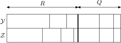 Figure 1
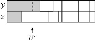 Figure 2
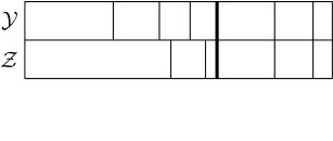 Figure 3
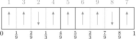 Figure 4
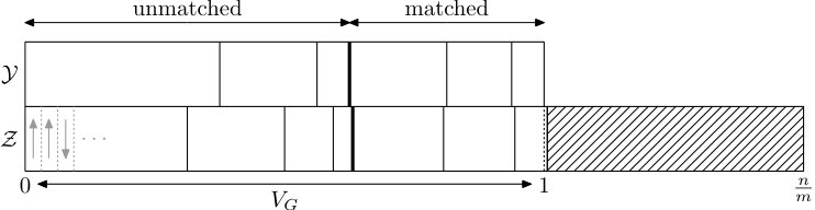 Figure 5
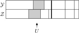 Figure 6
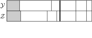 Figure 7
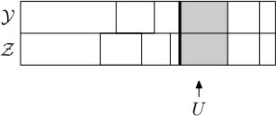 Figure 8
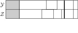 Figure 9
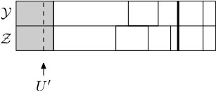 Figure 10
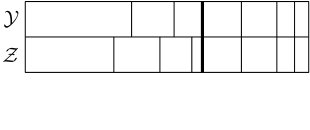 Figure 11
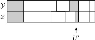 Figure 12
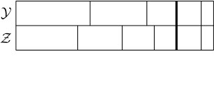 Figure 13
 Figure 14
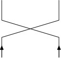 Figure 15
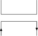 Figure 16
 Figure 17
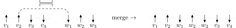 Figure 18
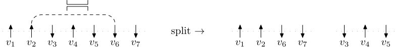 Figure 19
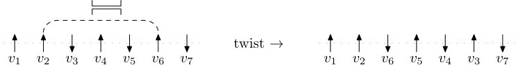 Figure 20
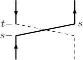 Figure 21
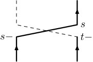 Figure 22
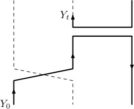 Figure 23
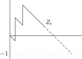 Figure 24
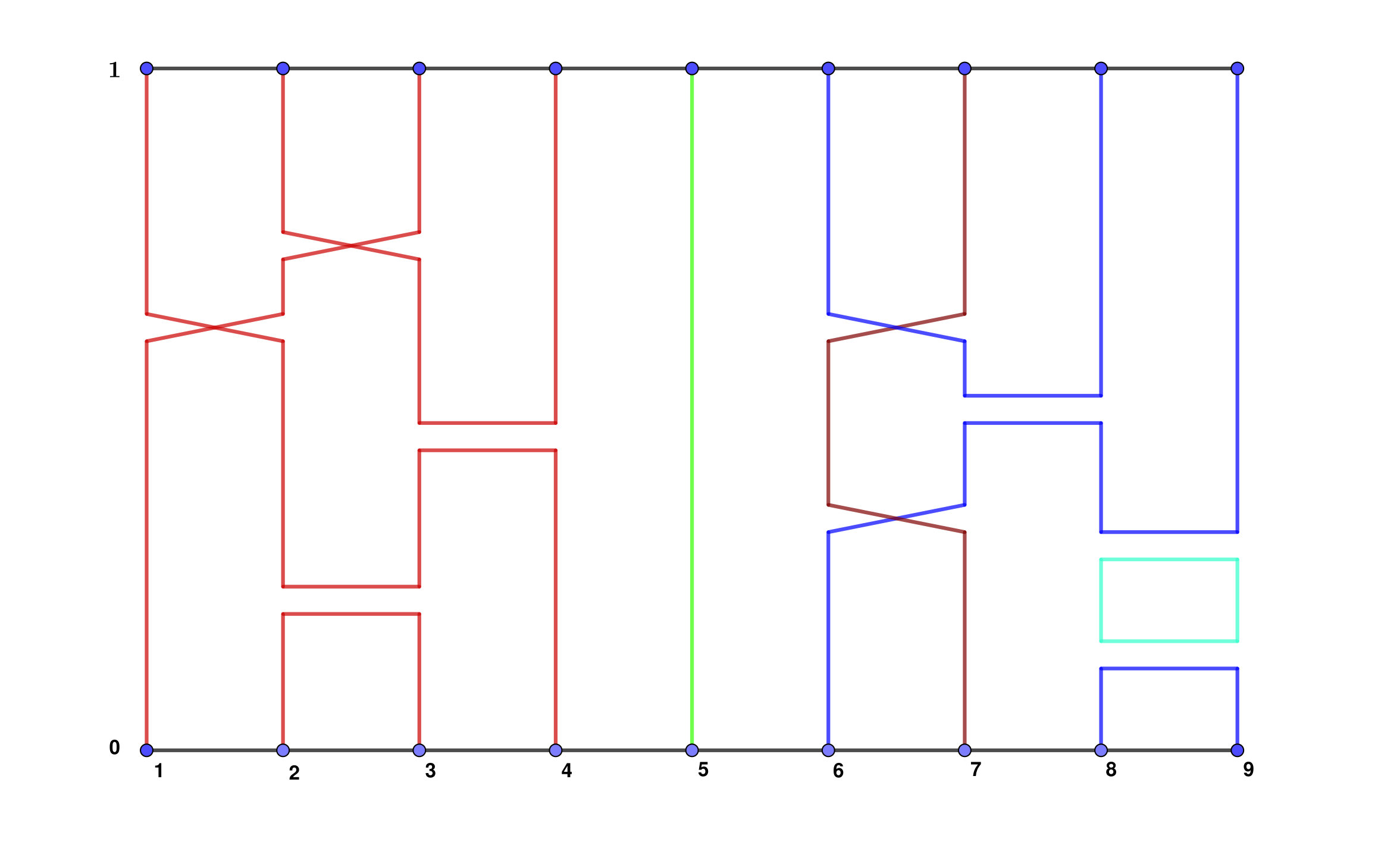 Figure 25
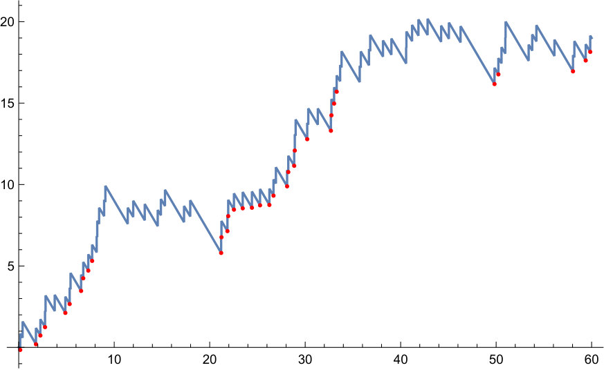 Figure 26
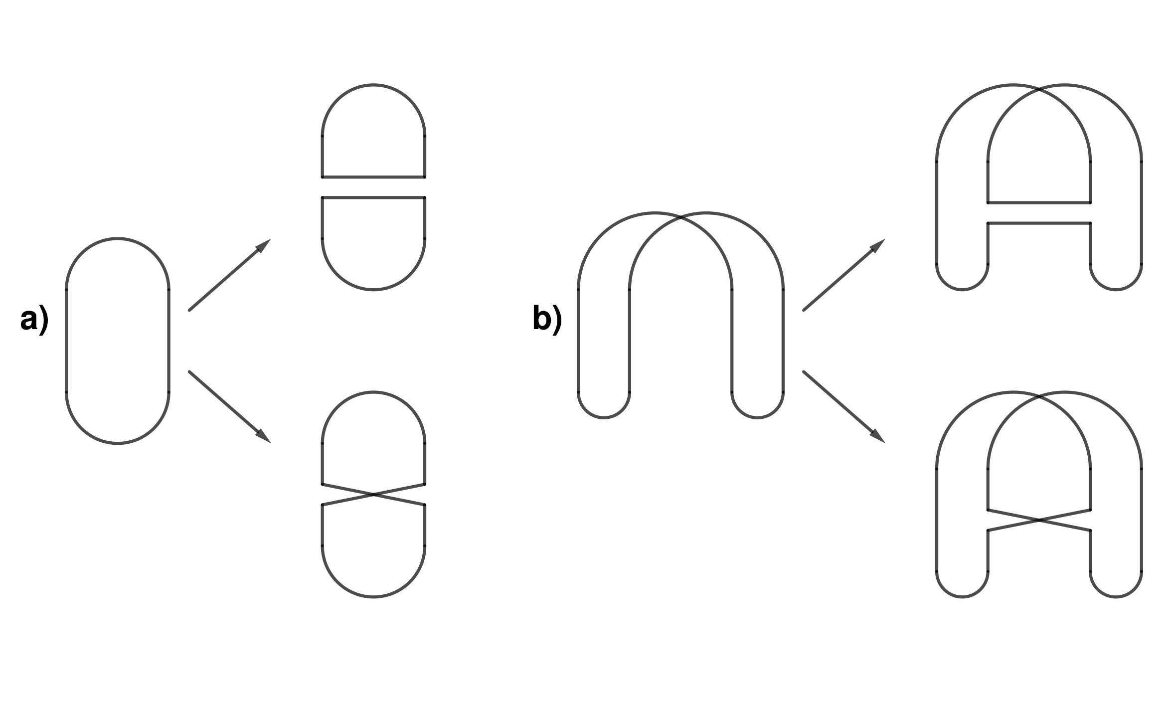 Figure 27
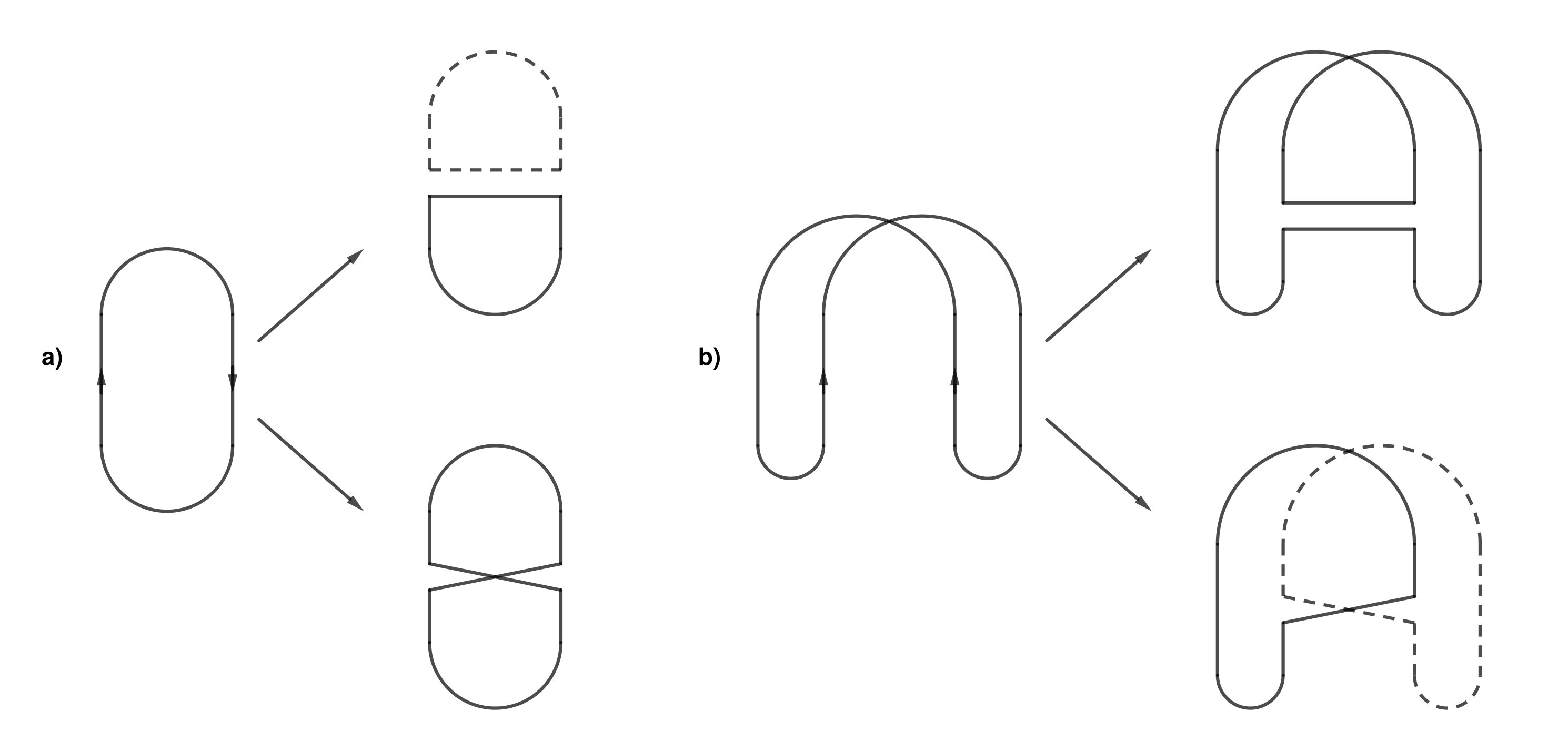 Figure 28
Peer Reviews
No public reviews on file for this paper yet. If you reviewed it on a platform where reviews are public (OpenReview, ICLR, NeurIPS, ICML), you can paste yours below so the community can read it here.
Videos
No videos yet. Explain this paper in a talk, walkthrough, or lecture? Add one.
The interchange process with
reversals
on the complete graph
J. E. Björnberg1
1Department of Mathematics, Chalmers University of Technology and the University of Gothenburg, Sweden
,
Michał Kotowski2
2Institute of Mathematics, Faculty of Mathematics, Informatics, and Mechanics, University of Warsaw, Banacha 2, 02-097 Warsaw, Poland
,
B. Lees3
3Fachbereich Mathematik, Technische Universität Darmstadt, Germany
and
P. Miłoś4
4 Institute of Mathematics of the Polish Academy of Sciences, Warsaw, Poland
[email protected], [email protected]
[email protected], [email protected]
Abstract.
We consider an extension of the interchange process on the complete graph, in which a fraction of the transpositions are replaced by ‘reversals’. The model is motivated by statistical physics, where it plays a role in stochastic representations of xxz-models. We prove convergence to PD() of the rescaled cycle sizes, above the critical point for the appearance of macroscopic cycles. This extends a result of Schramm on convergence to PD(1) for the usual interchange process.
Contents
1. Introduction
Recent years have seen a growing interest in the cycle structure of large random permutations. A major example is the interchange process, or random-transposition random walk. One motivation for studying this process is that it plays a key role in a stochastic representation of the most important quantum spin system, the ferromagnetic Heisenberg model. This representation was developed by Tóth in the early 1990’s [23] (after an earlier observation by Powers [20]).
At about the same time, a closely related stochastic representation was discovered for the anti-ferromagnetic Heisenberg model, by Aizenman and Nachtergaele [2]. Very roughly speaking, in the ferromagnetic Heisenberg model the interaction between neighbouring electrons behaves like a transposition of the spins. In the antiferromagnetic model the interaction involves a ‘reversal’, which Aizenman and Nachtergaele depicted as on the right in Figure 1.1.
In both cases, the stochastic representation of the spin system involves randomly placing these objects in the product of the graph with an interval. In the case of the ferromagnetic model, the relevant measure has transpositions appearing randomly at each edge, in the manner of independent Poisson processes. For the antiferromagnetic model, the structure is the same except that the transpositions are replaced by ‘reversals’ as on the right in Figure 1.1. Many quantities of interest for the spin systems, such as correlation functions, may be expressed using expected values of suitable random variables in these processes.
Recently, Ueltschi [25] explained that weighted combinations of the two processes described above also lead to representations of certain quantum spin systems (known as xxz-models). The relevant measure has independent Poisson processes on the edges as before, but the objects are now randomly chosen to be either transpositions or ‘reversals’, independently over the points of the process and with some fixed probability (see Figure 1.2). In this paper we study such a process defined on the complete graph. Our main result is that the correlation structure in this model, above a critical point, is described by a probability distribution on random partitions called the Poisson–Dirichlet distribution with parameter . To state our results more precisely, let us give the relevant definitions.
1.1. Definitions
We consider the complete graph on vertices. The vertex set is and the edge-set consists of all pairs of vertices . To each edge and vertex we attach a circle of circumference , which we denote by . We will sometimes identify with the unit interval . A configuration is a finite subset of E_{n}\times S^{1}\times\{\lower 1.42262pt\hbox{\includegraphics{interchange-1}},\lower 1.42262pt\hbox{\includegraphics{interchange-2}}\}, where \lower 1.42262pt\hbox{\includegraphics{interchange-1}},\lower 1.42262pt\hbox{\includegraphics{interchange-2}} are two possible marks which we call a cross and a bar, respectively. The collection of configurations is denoted . An element of the configuration is called a link and if is a link then we say that has a link at .
We will primarily be interested in configurations obtained as samples of a (marked) Poisson point process defined in the following way. Fix and . For each edge we consider a Poisson point process with intensity on , these Poisson processes being independent for different edges . This defines a configuration of unmarked links. The configuration is then obtained by assigning to each link a mark, independently of all other links, which is either a cross, , with probability , or a bar, , with probability . The probability measure corresponding to this point process will be denoted by (we consider to be fixed and it will be suppressed in the notation), and the corresponding expectation will be denoted by . We will refer to this process as the interchange process with reversals (the usual interchange process would correspond to taking ).
Such a configuration gives rise to a set of loops . We first give an informal description and then a more precise definition. For a fixed point the unique loop, , containing it is constructed by the following process. Starting from we move on the associated circle in the positive direction, i.e. after time we are at a point . If we encounter a point such that has a link at for some , then we traverse this link to . We then continue moving in the positive direction if the link was a cross, or in the negative direction if the link was a bar. Each time we encounter a link we follow this rule of traversing the link, reversing our direction if the link was a bar. Continuing until we arrive back at we have traced out a single loop, .
More formally, following [10, 25] we may define the loops as follows. A loop of length is a function such that, writing , the following properties hold:
- (1)
is injective and satisfies . 2. (2)
is piecewise continuous, and if it is continuous on the interval then and are constant on , with . 3. (3)
is discontinuous at the point if and only if has a link at for some , in which case . 4. (4)
If and with continuous on and but discontinuous at then for any and we have that if the link at is a cross and if it is a bar.
Loops with the same support but different parameterisations are identified. This means that the functions , and, for , are identified. From this description we can give a natural pictorial representation, see Figure 1.2.
A cycle is a sequence of vertices such that the points are visited by a single loop. Namely, suppose we start at a point and follow the loop , in either direction, until we return to the starting point. If we enumerate the successive visits to as then the corresponding cycle is
[TABLE]
Here the cycle has length , and the denote the direction in which we pass through the point , with corresponding to the positive direction () and corresponding to negative direction (). Note that the directions in a cycle are defined up to an overall reversal and that we made an arbitrary choice of the first vertex . It is also worth noting that not every loop gives rise to a cycle, see Figure 1.2. A fixed configuration of links, , has an associated set of cycles which we denote by .
1.2. Main result
Let be sampled from the measure . Consider the random graph where an edge is present between vertices and if there is at least one link on in . By the Erdős-Rényi theorem, if then the largest connected component of this graph, , has size approximately where is the positive solution to . (If the largest component has size smaller than and the same holds for the largest cycle.) Let denote the list of rescaled cycle sizes, ordered by decreasing size (we make it into an infinite list by appending infinitely many 0’s). Our main result is the following.
Theorem 1.1**.**
Let and . Let be sampled from the corresponding measure . As the law of converges weakly to the Poisson–Dirichlet distribution PD().
More precisely, we will show that for given and there exists such that for there is a coupling of the interchange process with reversals with a PD() sample such that
[TABLE]
Note that this result holds for any .
The Poisson–Dirichlet distribution with parameter , PD(), can be defined via the ‘stick-breaking’ construction as follows. Let be independent Beta() random variables, thus for . We construct a random partition of using the by letting and . We can think of constructing by progressively breaking off pieces of , with the removed piece being a fraction of what remained after pieces had been removed. The law of the partition is called the GEM() distribution. The PD() distribution is obtained by sorting the in order of decreasing size.
Returning to the context of Theorem 1.1, let us comment on the case (only crosses allowed) which is excluded by our result. This is the (usual) interchange process, and was considered on the complete graph in a famous paper by Schramm [21]. To be precise, he considered the closely related process where the configuration is obtained by placing the crosses successively one after the other, uniformly and independently at each step. Viewing the crosses as transpositions, as above, the process is a random-transposition random walk on the set of permutations of objects. In this case Schramm proved that, when the number of transpositions exceeds for , then the rescaled cycle sizes of the resulting random permutation converge in distribution to PD(1).
The main tool in Schramm’s argument was a coupling with a split-merge process which has PD(1) as an invariant distribution. Roughly speaking, the important feature is what happens to an existing cycle when a uniformly chosen transposition is applied. If the transposition transposes two points which belonged to different cycles then those cycles merge; if they belonged to the same cycle then the cycle is split. A similar principle applies to the loops, which on the addition of another cross to either merge, if the ends are in different loops, or split, if both ends are in the same loop (Figure 1.3).
Now we may explain how the case is different from , and why we get PD() rather than PD(1). The key point is that the presence of bars () introduces changes of orientation within the loops. This means that on adding a link (cross or bar) with both endpoints in the same loop, this loop will not always split. Whether or not the loop splits depends on the orientation of the loop at the points where the new link is placed. Specifically, if the link is a cross then a split occurs if and only if the orientation is the same; if it is a bar then the opposite applies. The situation is depicted in Figure 1.3.
Intuitively, when one would expect large loops to encounter many bars. Hence a uniformly chosen pair of points on a large loop (with the same -coordinate) should have probability close to of having the same orientation, meaning that the probability of splitting is close to . The corresponding split-merge dynamics, where proposed splits occur with probability , has PD() as its invariant distribution.
1.3. Outline and related works
In order to prove Theorem 1.1 we need three ingredients. Firstly, we need that with high probability (converging to 1 as ) there are cycles of size , and that these large cycles occupy almost the entire giant component . This is proved in Section 2 by a straightforward adaptation of arguments in [21]. Secondly, we need that in large cycles roughly half of all vertices are passed through in the positive direction () and roughly half in the negative direction (). In fact, we need the stronger statement that the large cycles are ‘well-balanced’, namely: one may partition them into much smaller segments such that each segment consists of roughly half and half (ruling out, for example, a situation in which a cycle of size consists of a block of vertices passed in direction followed by a block of vertices with direction ). This is the main novel contribution of the present paper, and is the content of Section 4. In proving this result we rely on a process which we call the exploration process, which we study in Section 3. Thirdly, we show that Schramm’s coupling, when combined with the previous two ingredients, can be adapted to couple a PD() sample with such that the two samples are close. This appears in Section 5.
We now briefly summarise some other related works apart from Schramm’s paper [21]. First note that interchange processes, with reversals () or without (), can be defined on more general graphs, by placing independent Poisson processes of links on the edges of the graph. Most papers dealing with graphs other than the complete graph have studied the question of whether there can be large cycles. The case when the graph is a hypercube, and , has been investigated by Kotecký, Miłoś and Ueltschi [15]. The case of Hamming graphs, also for , has been investigated by Miłoś and Şengül [17] and by Adamczak, Kotowski and Miłoś [1]. In the case when the graph is an infinite tree one may ask about the occurrence of infinite cycles. For this question was investigated by Angel [3] and by Hammond [12, 13]; and for by Björnberg and Ueltschi [8] as well as Hammond and Hegde [14].
As mentioned above, the original interest in the process was due to its connections with quantum spin systems. When the measure defining the process is given an additional weighting of for , the loop-model is essentially equivalent to a spin system on the same graph. This was first proved by Tóth [23] in the case (spin- Heisenberg ferromagnet for ) and Aizenman and Nachtergaele [2] in the case (Heisenberg antiferromagnet, provided the graph is bipartite). This connection was extended to the case by Ueltschi [25]. From a probabilistic point of view, any makes sense. Such models have been considered on trees [9, 5] and on the Hamming graph [1]. In very recent work there has been some limited progress in the direction of establishing Poisson–Dirichlet structure in these and related loop models [4, 7]. For the Heisenberg model ( and ) on the complete graph, the critical point for the appearance of cycles of diverging length was established already in the early 1990’s by Tóth and by Penrose [18, 22].
Acknowledgements
The research of JEB is supported by Vetenskapsrådet grant 2015-05195. BL gratefully acknowledges support from the Alexander von Humboldt Foundation. JEB and BL also gratefully acknowledge support from Stiftelsen Olle Engkvist Byggmästare. MK acknowledges support from the National Science Centre, Poland, grant no. 2015/18/E/ST1/00214. PM is supported by the National Science Centre, Poland, grant no. 2014/15/B/ST1/02165. We thank Radosław Adamczak for useful discussions about this project.
Notation
[TABLE]
2. Large cycles
In this section we show that, for , with high probability there are cycles of length of order . The precise statement appears in Lemma 2.4 at the end of the section. The argument is a minor adaptation of Schramm’s [21, Section 2].
As in [21], we will actually work not with configurations sampled from the Poisson measure , but instead with configurations constructed sequentially one link at a time. Given any configuration , note that the set of cycles only depends on the relative order of the links of as well as their position relative to , but not on their precise -coordinates. Given , let us order its elements (links) with respect to the -coordinate, namely we write , with (we can assume that there are no distinct links with , since under this occurs with probability ). We denote by the ordered list of links with -coordinates suppressed. With a slight abuse of terminology we will also refer to the entries of as links. As noted above, is a function of only, hence we may write .
In the rest of this section we will work with a random obtained by sequentially laying down a fixed number of random links. More precisely, first let be chosen uniformly from the edge-set and let m_{1}\in\{\lower 1.42262pt\hbox{\includegraphics{interchange-1}},\lower 1.42262pt\hbox{\includegraphics{interchange-2}}\} be chosen independently of , with probability for . Next, given the first links , we select uniformly from and the mark m_{s+1}\in\{\lower 1.42262pt\hbox{\includegraphics{interchange-1}},\lower 1.42262pt\hbox{\includegraphics{interchange-2}}\}, with probability for , independently of each other and of the previous choices. Write and let denote the set of cycles after steps. Note that, if is taken to be Poisson-distributed with mean , then is equal in distribution to for sampled from . Due to concentration properties of the Poisson-distribution, there is very little difference between for on the one hand, and for sampled from on the other. We will not make this statement more precise at this point, deferring this to later (see Section 5.3).
We now describe in detail the effect that appending the next link to has on the cycles, that is, the transition . See Figures 2.1, 2.2 and 2.3 for illustrations in the case when m_{s+1}=\lower 1.42262pt\hbox{\includegraphics{interchange-2}}.
For we write for the reversed arrow. We have the following:
- •
If the endpoints of are in different cycles of then those cycles merge.
- •
If the endpoints are in the same cycle then the result depends on the mark in the following way. Let us assume that and that where . Without loss of generality (since directions are defined up to an overall reversal) we may assume that .
- –
If m_{s+1}=\lower 1.42262pt\hbox{\includegraphics{interchange-1}} is a cross then splits if and only if ; in this case the two resulting cycles and are given by:
[TABLE]
On the other hand, if then is not split; instead it is modified into where
[TABLE]
- –
If m_{s+1}=\lower 1.42262pt\hbox{\includegraphics{interchange-2}} is a bar then splits if and only if ; in this case the two resulting cycles and are given by:
[TABLE]
On the other hand, if then is not split but modified into where
[TABLE]
Note that the edge may be selected by first choosing uniformly from and then uniformly from . In particular we see that, just as in [21, Lemma 2.1], we have:
Lemma 2.1**.**
In the step from to , the probability that some cycle is split into two cycles, with at least one containing at most vertices, is at most .
Building on this, and replicating the arguments of Schramm [21], we obtain the following sequence of lemmas. Lemma 2.2 is proved exactly as [21, Lemma 2.2]. Lemma 2.3 is a version of [21, Lemma 2.3] and is proved in a similar way, see [1, Lemma 5.1] for details. Briefly, the reason that these results hold exactly as in [21] is that, firstly, if the endpoints of are in different cycles then those cycles always merge, and, secondly, the cycle may or may not split if the endpoints are in the same cycle. This means that both the upper bounds on the probability of splitting, as well as the lower bounds on the probability of merging, are identical to [21]. This is all that we need.
In the following statements we consider a random graph with vertex set obtained by placing an edge between a pair , , if in there is at least one link , , such that . We write for the set of vertices in connected components of containing at least vertices. Similarly, we write for the set of vertices belonging to cycles of which are of length at least .
Lemma 2.2**.**
For any ,
[TABLE]
Lemma 2.3**.**
Let , , and be such that . Assume that the following conditions hold in the transition from to :
- (1)
there exists such that for any , we have
[TABLE] 2. (2)
there exists such that for any and any two cycles we have
[TABLE]
Then there exist , depending only on , such that if
[TABLE]
then
[TABLE]
Note that in our case condition (1) is satisfied because of Lemma 2.1 and condition (2) is trivially satisfied. In notation of [1, Lemma 5.1] this corresponds to taking the stopping time , i.e. conditions (1) and (2) hold for all times . The lemma states that if, at some time , enough vertices are in reasonably large cycles (size ) then at some carefully chosen later time most of these vertices will be in cycles of size of the order . Here one should think of as approximately and of for some . Then by the Erdős–Rényi theorem, hence by Lemma 2.2 also . Note that if then is of the order , thus for any and we may select such that .
The final result of this section paraphrases [21, equation (2.4) in Lemma 2.4]. It tells us that most of the vertices in (the largest connected component in ) belong to large cycles. The proof is precisely as in [21] as the only appeal to the particular structure of the cycles is through invoking the previous lemmas, which all hold as in [21].
Lemma 2.4**.**
Fix , take , . There is some such that for any , if is large enough we have
[TABLE]
3. Exploration processes
An important tool in proving Theorem 1.1 is the exploration process, which we will define in this section. The exploration process is sometimes also called the cyclic-time random walk, see e.g. [13, 14]. It will allow us to uncover the loop containing some specified point at the same time as we uncover the configuration itself. We will also define a process which we call the simple exploration process which is easier to analyse and which may be coupled with the exploration process. In this section we work with a random sampled from the Poisson measure for some fixed (the definitions will make sense for all ). Recall that is fixed throughout.
3.1. Definitions
The exploration process will be denoted and takes values in . Recall that we identify with the unit interval using periodic boundary conditions. We will write . Let be an initial direction and set , where . The process starts by traversing at unit speed in the direction specified by , meaning that , and . This continues until it either encounters a link of , or it returns to its starting point, i.e. . If a link is encountered first, say at time and with other endpoint in , then the process jumps to and proceeds in a direction which depends on whether the link was a cross or a bar. That is, we set and and if the link was a cross or and if the link was a bar. We define the process to be right-continuous (càdlàg). The process proceeds in this way, traversing links and adjusting its direction accordingly, until it returns to the starting point . We let
[TABLE]
be the time when this happens. After this time the process is no longer useful to us, but to be definite we declare that the process continues by repeating itself periodically after time . Note that at time , the loop containing has been fully discovered.
Let us consider those links that, by time , have been traversed by at least once. Some of them have been traversed only once, others twice (no link can be traversed more than twice before time as this would entail visiting a previously visited point ). We say that a link is discovered at the time of its first traversal, and backtracked on its second traversal (if traversed twice). Let denote the number of times the exploration , started at and run for time , has discovered a link (‘jumped’). Let denote the number of times it has traversed some link, including backtracking. Thus for all . Next, define the history of as
[TABLE]
This is the set of points in visited by up to time . Finally, let denote the natural filtration of the exploration process, namely \mathcal{F}_{t}:=\sigma\big{(}(X_{s})_{0\leq s\leq t}\big{)}, and .
When is randomly sampled from the Poisson measure we may, thanks to the memorylessness of Poisson processes, construct (part of) itself simultaneously with . This fact is central to our approach. We formulate the construction as a proposition. In the following result we will be using a Poisson process on and we will say that rings at time if it has an arrival at that time.
Proposition 3.1** (Construction of the exploration process).**
Let , and . Consider the following independent objects:
- •
a Poisson process with intensity ,
- •
a sequence of i.i.d. random variables distributed uniformly on ,
- •
a sequence of i.i.d. random variables taking values and satisfying .
When has law , then the law of the exploration , started at , may be constructed as follows:
- (1)
The process starts at and initially only changes, according to . 2. (2)
Whenever rings, say at time , we inspect vertex . We have two cases:
- (a)
If or then nothing happens and the process continues on, i.e. . 2. (b)
Otherwise we set and then evolves according to . 3. (3)
Between successive rings of the process may backtrack across previously discovered links. More precisely, a backtrack occurs at time if there exists another time such that and either:
- •
, in which case we set , or
- •
, in which case we set .
See Figure 3.1.
The construction of Proposition 3.1 is fairly standard and has been used previously in for example [1, 13, 14], hence we do not give a proof. Let us however draw attention to the condition that, when or , then the jump proposed by is canceled. This means that cannot jump to a previously visited point , which effectively amounts to a reduction of the intensity of jumps (see Lemma 3.5 below).
The main difficulty in analysing is that it may discover a new link which takes it to a previously visited copy of , i.e. it may jump at time to a point satisfying for some . We refer to this as jumping to the history. In this case has already been partially explored, making quite difficult to analyse directly.
To get around this problem we introduce what we call the simple exploration process , which is easier to analyse and (on time intervals which are not too long) can be coupled with the exploration process . Roughly speaking, the idea is that for we replace the vertex set with an augmented vertex set , where the -coordinate increases on discovering a new link. The interpretation is that each newly discovered link brings us to a ‘fresh’ circle .
Below we give a detailed definition. Notice that the wording is very similar to Proposition 3.1, the main difference being what happens at the jump times of .
Definition 3.2** (Simple exploration process).**
Let , and . We construct the simple exploration process as a càdlàg process, using the following independent objects:
- •
a Poisson process with intensity ,
- •
a sequence of i.i.d. random variables distributed uniformly on ,
- •
a sequence of i.i.d. random variables taking values and satisfying .
Using these sources of randomness the process is constructed as follows:
- (1)
The process starts at and initially only changes, according to . 2. (2)
Whenever rings, say at time , we inspect vertex ; we have two cases:
- (a)
If then nothing happens and the process continues on, i.e. . 2. (b)
If we set and then evolves according to . 3. (3)
Between successive rings of the process may backtrack across previously discovered links. Now there is only one possibility for backtracking: a backtrack occurs at time if there exists another time such that and , and then we set .
As we did for we let
[TABLE]
be the first time at which the simple exploration process arrives back at the starting point. Note that , in contrast to , may take the value , see Proposition 3.4. If we assume that the process stops evolution after .
For we define the history by
[TABLE]
By slight abuse of terminology, if for some then we say that started at . As for we denote by (respectively, ) the number of times the simple exploration process has discovered (respectively, traversed) a link when started at and run for time . We denote by the restriction of to , that is if then .
The important point which makes simpler to analyse than is that, each time discovers a new link (i.e. rings and ), we set to a previously unused value, namely . This means that , by construction, can never jump to its history. Crucially, it does still backtrack across previously discovered links.
3.2. Coupling with the simple exploration process
The following lemma shows that when is randomly sampled from , one can couple the exploration process and the simple exploration process so that they evolve in the same way on a sufficiently short time scale. One should think of .
Lemma 3.3** (Coupling with the simple exploration process).**
Fix . Let be the exploration process and let be a stopping time with respect to the filtration such that jumps to a previously unvisited vertex at time . Conditionally on , there exists a coupling of a process with a process such that:
- (1)
The process is a simple exploration starting from where . 2. (2)
\mathbb{P}\big{(}\big{\{}\tilde{X}_{t}\big{\}}_{t\geq 0}\in\cdot\mid\bar{\mathcal{F}}_{\sigma}\big{)}=\mathbb{P}\big{(}\left\{X_{t+\sigma}\right\}_{t\geq 0}\in\cdot\mid\bar{\mathcal{F}}_{\sigma}\big{)}. 3. (3)
\mathbb{P}\big{(}\forall_{t<\tau^{Y}\wedge T}\;\tilde{X}_{t}=Y_{t}^{\prime}\mid\bar{\mathcal{F}}_{\sigma}\big{)}\geq 1-4\beta T(\mathcal{J}^{X}_{\sigma}+\beta T)/n.
If at some time we have then we consider the coupling as failed at time . The history of is defined as in (3.2).
Proof.
In the following we write simply for . We will construct \big{\{}\tilde{X}_{t}\big{\}}_{t\geq 0} using the same sources of randomness as for , namely the same , and as given in Definition 3.2. We write .
- (1)
The process starts at and initially only changes, by . 2. (2)
Whenever rings, say at time , we inspect vertex ; we have two cases:
- (a)
If or then nothing happens and the process continues on. 2. (b)
Otherwise the process jumps to . 3. (3)
Between successive rings of the process may backtrack as before, using links of both and .
It follows from Proposition 3.1 that and have the same distribution, giving statements (1) and (2) from the lemma.
For the proof of (3), let
[TABLE]
be the sets of vertices visited by up to time and by up to time , respectively. We define
[TABLE]
Until time the processes and are equal, thus
[TABLE]
Each time when rings there is a chance that . This has probability at most the number of previously visited vertices divided by . Since the number of visited vertices cannot exceed the number of discovered links by more than 1, we get
[TABLE]
where in the last equality we used that has Poisson distribution with mean . Since this gives the claimed bound on \mathbb{P}\big{(}\forall_{t\leq\tau^{Y}\wedge T}\tilde{X}_{t}=Y_{t}^{\prime}\big{)}. ∎
3.3. Properties of the exploration processes
Next we present some basic properties of the processes and , starting with the simple exploration .
First note that , the number of links discovered by time , is a Poisson process with rate , stopped at time (at which time itself terminates). It will be convenient to extend this process beyond time . For this purpose we let denote a Poisson process of rate which agrees with up to time .
Many relevant properties of can be understood in terms of the process given by . For example, if hits then this corresponds to returning to its starting point, that is to say we have that . To see this, note that counts the number of copies of that has visited by time . If then , which means that the total time spent equals the number of ’s visited. Hence at this time has explored the entirety of each copy of it has visited, meaning that it must have returned to its starting point. See Figure 3.2
Note that implies that almost surely. We define a sequence of random times which we call frontier times , as well as processes , as follows. First, we let and . Next, we let be the time when attains its global minimum (note that as almost surely, this time is almost surely finite). This is necessarily a jump time of (equivalently, of ) but it is not a stopping time. Inductively, is the time when attains its global minimum. We also write for the time spent between successive frontier times. See Figure 3.3 for a sample trajectory of the process with frontier times marked.
In terms of the simple exploration , the frontier times play the following role. Recall that the jump times of are exactly the times when discovers a new link. The frontier times are the times when discovers a new link which is never backtracked.
Proposition 3.4** (Survival and increments of the simple exploration).**
Let and write .
- (1)
We have that , where is the unique positive solution of . 2. (2)
There exists such that
[TABLE] 3. (3)
Conditionally on , the sequence \big{\{}\big{(}\Delta_{k},(Z^{(k)}_{t})_{0\leq t<\Delta_{k}}\big{)}\big{\}}_{k=0}^{+\infty} is i.i.d. 4. (4)
There exists such that for any
[TABLE]
The proof is based on well-known properties of Poisson processes, for completeness we provide details in Appendix A. The first two parts of the proposition tell us that the simple exploration either continues indefinitely, or it closes ‘quickly’. Intuitively, the former scenario parallels the situation when the (true) exploration process explores a large cycle. The other two parts tell us that, conditionally on ‘surviving’, the frontier times are renewal times, and the renewal intervals are typically short.
We now turn to discussing some properties of the exploration process . Recall that \mathcal{J}^{X}_{t}:=\#\{s\leq t\colon\textrm{Xs}\}. Let
[TABLE]
denote the total number of vertices visited by up to time , and let denote the event that no more than vertices have been visited up to time . Note that and that where is the Poisson process of rate in Proposition 3.1. From this and a simple argument using Laplace transform we see that
[TABLE]
In particular, if then for some .
By we will denote the set of vertices available to the exploration at time by means of a new jump, i.e. if , otherwise if then
[TABLE]
Recall that a counting process is a nondecreasing, integer valued càdlàg stochastic process starting at zero and with jumps equal to one. Let be an -adapted counting process. We will say that a nonnegative process is an intensity of if is -progressively measurable, a.s. for all , and the process is an -martingale.
Lemma 3.5** (Intensity of jumps).**
The processes and are counting processes with intensities , given respectively by
[TABLE]
In particular, on the event we have .
A proof of this rather intuitive statement may be found (in a more general setting) in [1, Lemma 3.7]. The following lemma also appears in a more general form in [1, Lemma A.2], we include its proof here for the sake of completeness.
Lemma 3.6**.**
Suppose is a counting process with intensity and let . Let , be stopping times such that . Let . Then we have
[TABLE]
Proof.
Consider any with positive probability and the process , which is a counting process with intensity with respect to the filtration . Let . We have . Let be a Poisson process with intensity such that almost surely (see [1, Theorem A.1] and references there). We get
[TABLE]
Using the form of the Laplace transform of and Chebyshev’s inequality we obtain
[TABLE]
where in the second step we have used the elementary inequality valid for . Thus we get
[TABLE]
for arbitrary of positive probability, which implies the lemma. ∎
Corollary 3.7** (Visits to previously unvisited vertices).**
Let be a stopping time with respect to the filtration of the exploration process and let be the first time after when makes a jump to a previously unvisited vertex. For any on the event we have
[TABLE]
Proof.
By definition of , between times and there are no jumps to previously unvisited vertices. In particular implies that and that holds. Thus Lemma 3.5 implies, with being the intensity of and , that then . Applying Lemma 3.6 with , and easily gives the desired estimate. ∎
4. Balance
This section contains the main work of the paper. The goal of the section is to prove that large cycles are ‘balanced’ in the sense that they contain roughly equal numbers of vertices passed in the directions and . In fact we show that, with high probability, in a cycle which is at least long each segment of consecutive vertices is balanced in this sense. Throughout the section we work with a random sampled from the Poisson measure for some fixed (recall that is fixed).
We start by introducing some notation. Given , and , let us write for the cycle containing . Without loss of generality we may assume that and that . Under these assumptions, we let
[TABLE]
denote the set of the first vertices of following . Note that if the cycle containing has length smaller than then . We further let
[TABLE]
denote those vertices in which are passed in the same, respectively opposite, direction as . Finally we define the balance of the segment of length after in the loop, as
[TABLE]
The main result of this section is the following proposition, which tells us that is typically of much smaller order than .
Proposition 4.1** (Segments of cycles are balanced).**
Let . There exist such that for all and for any , we have
[TABLE]
This says that cycles of length at least are very likely to have balance . Cycles containing fewer than vertices may possibly be unbalanced, but this does not concern us. A key feature of this result is that the upper bound kills any polynomial in , making it possible to use quite crude union bounds later in the proof of Theorem 1.1. Also note that the bound is claimed to be uniform in for any . This will allow us to derive a version of the proposition stated above where we ‘remove’ a deterministic number of links from , which will be important for the coupling with PD() in Section 5.
To formulate the last claim precisely, recall the notation for the ordered list of links of , and note that , , , and all depend on only. Also recall that, for , we write for the sequence of the first links. If is a random variable which only depends on the relative order of links in we write for its value on any link configuration with the same relative order.
Proposition 4.2**.**
Let and . For write
[TABLE]
There exist such that
[TABLE]
The proofs are given at the end of the section, after several preparatory results.
4.1. Winding processes
Recall the notation and for the exploration and simple exploration, in particular that indicates the direction of motion. We will use superscripts and on to distinguish between the two processes. Define the winding processes and by
[TABLE]
Thus increases at rate when the process travels in the positive direction, otherwise it decreases at rate , and the same is true for .
To prove Proposition 4.1 we will first estimate , and then transfer these estimates to . In order to estimate we will use the coupling of and introduced in Lemma 3.3, together with the following estimate on :
Proposition 4.3** (Winding of the simple exploration process).**
Let . There exist such that for any , and we have
[TABLE]
where .
Proof.
Fix . We use Proposition 3.4 and the notation therein, we also write . For lighter notation, within this proof let .
At each frontier time the process jumps, meaning that discovers a new link. We let and let be the subsequence consisting of the times at which the link is marked as a bar (i.e. in the notation of Definition 3.2). As the choice of markings is independent of , using Proposition 3.4 we conclude that form an i.i.d. sequence under , satisfying
[TABLE]
for some . Also, the increments are independent under .
Now, the key observation is that we have the equality in distribution
[TABLE]
because upon crossing a bar the winding processes changes its orientation. Using these facts we infer that for any
[TABLE]
are symmetric random variables with being independent. Moreover, by and (4.1) they have exponential tails.
Let us set for some to be chosen later. We consider the cases and separately. If then we can cover with the intervals for . As is continuous in , we can replace the supremum of by maximum. The maximum can then be bounded by the maximum at endpoints plus the maximum increment over all the intervals . The maximum increment on is in turn bounded by the length . We thus get
[TABLE]
The first of these two terms can be bounded by applying a union bound and Etemadi’s inequality [6, Thm. 22.5], giving
[TABLE]
where we have used that are i.i.d. By symmetry of and Markov’s inequality we have for any that
[TABLE]
For small enough the Laplace transform is finite, since the ’s have exponential tails. Using that we see that there exist such that if then . Setting with chosen large enough so that we get (using and )
[TABLE]
with .
For the second term on the right in (4.1) we recall that the ’s have exponential tails. As , we thus obtain for some
[TABLE]
Finally, by standard large deviation considerations for i.i.d. variables we have
[TABLE]
for some , provided we choose large enough so that the mean of the sum above is larger than .
This proves the claim for any fixed . The uniformness over such follows since the upper bound can be chosen as a continuous function of . ∎
In order to compare with we need to keep track of how many times the exploration passes level . To this end we make the following definitions. Denote by (respectively, ) the number of times (respectively, ) passes through when started at moving in the positive direction () and run for time . We will write (respectively, ) when the starting point is not ambiguous. Recall the definition of given right after (3.4).
Proposition 4.4** (Winding and the number of visited vertices).**
For any and any we have
[TABLE]
Moreover, there exists and such that
[TABLE]
where as usual .
Proof.
The proofs of (4.2) for and are the same. We write and , omitting , , and in order to simplify the notation.
Define a sequence of times and, for ,
[TABLE]
We first claim that for we have
[TABLE]
Indeed, at time the exploration passed and if it passes 0 again without traversing a link this means that it has completed a full lap on one copy of . From (4.4) we deduce that
[TABLE]
Let be such that . Then
[TABLE]
as claimed.
Now we turn to (4.3). Recall from Proposition 3.4, and the discussion preceding it, the notation and as well as the notion of frontier times. Let us use the term return times for the jump times of which are not frontier times, and return links for the corresponding links traversed by . Observe that , where denotes the number of return links which have been backtracked by up to time . This is because does not visit its own history other than by backtracking, hence between discovering a return link and backtracking it must complete at least one circle.
Let denote the total number of return times of . By Proposition 3.4, conditionally on the sequence is a renewal-reward process, and by the basic renewal-reward theorem [11, Theorem 10.5] it thus follows that
[TABLE]
The result (4.3) follows from , which is easily checked. For example, it suffices to check that . Letting denote the jump times of and using that we get
[TABLE]
∎
We now come to the key technical result of the paper, an upper bound on when explores part of a large cycle. At the same time we also provide a lower bound on since the proof follows a similar structure.
Proposition 4.5** (Winding for the exploration process is small).**
Let , and consider the exploration started at an arbitrary point . There exist such that for any we have
[TABLE]
Moreover, we have for some
[TABLE]
Before giving the proof we outline the main ideas. We want to use the coupling of the exploration process to the simple exploration process from Lemma 3.3, as well as the concentration result for the latter process, Proposition 4.3. To get good concentration we will decompose into many shorter time intervals of length approximately each. On each we will wait for a ‘good’ coupling with a simple exploration: first we wait until the exploration jumps to a new vertex so we can start a coupling, then we check if the simple exploration survives indefinitely, which it does with probability . If so, we can apply Proposition 4.3 in this interval. If not, then we repeat the procedure, waiting for a jump of to a new vertex and looking at the coupled simple exploration. Typically we only need to perform this a small number of times until we get a coupling with a simple exploration which survives.
Let us make these ideas formal and introduce the setup that will be used in the proof. Set . We define where , . Writing , we decompose
[TABLE]
Fix . Let us first analyse the change of the winding process on one interval . To this end we will define two sequences of times and as well as a sequence of simple explorations . The will form a non-decreasing sequence, taking values in , and will be defined so that, for and as long as , the process jumps to a new vertex at time . For such , the process is defined to be an independent copy of a simple exploration, coupled with as in Lemma 3.3, starting at time . The possibility signifies that we have finished with the interval and must move on to the next one.
We now define the times and . First we set . Next, for we set
[TABLE]
where is the time when terminates (returns to its starting point). Note that if then . In particular, this will occur if . In this case we do not need to define Also note that, since the coupling of with entails constructing both processes using the same sources of randomness, we may work with the as if they are adapted to the filtration of , even though they are defined in terms of .
In words, these definitions mean that, firstly, is a simple exploration coupled with , started at time , the first time in that jumps to a new vertex. This coupling is then run either for the remaining time in , or until returns to its starting point (after time ). For , if the simple exploration has returned to its starting point, at time , then we wait until jumps to a new vertex again. We call the time when this occurs and we begin a new coupling with a simple exploration, , from the location of at this time.
Let
[TABLE]
The first possibility, , means that at attempt number the coupled simple exploration survives (and is the first one with this property). The other possibility, that but , means that after time the exploration never jumps to a new vertex until the end of the interval . Included in this possibility is the case when closes the loop before jumping again. Intuitively, is the number of attempts at coupling with a simple exploration which survives, until we either succeed or run out of time.
We now turn to the proof of the proposition.
Proof of Proposition
4.5.
Fix . We first show (4.5) for this . Recall the definition of the event given above (3.7). First note that it suffices to show that
[TABLE]
satisfies the claimed bound, due to (3.7). Also note that for .
Consider the interval , the stopping times and the variable from the preceding discussion. Keeping fixed for now, we will drop it from the superscript on , and . We claim that, under , the random variable is stochastically dominated by a geometric distribution with parameter , that is to say,
[TABLE]
Here is the survival probability of a simple exploration, see Proposition 3.4. The claim is easily established by induction, using
[TABLE]
and
[TABLE]
We now show that there exist constants , uniform in and in , such that for all , on the event we have
[TABLE]
First we establish that there are such that for any and any , on we have
[TABLE]
Indeed, for any we have , so
[TABLE]
The second term is at most , for some , by (3.5) from Proposition 3.4. To estimate the first term, note that together with implies that , in particular does not visit previously unexplored vertices for time at least after . Thus
[TABLE]
By Corollary 3.7 the probability is at most for some , which together with the previous estimate proves (4.8).
Now note that
[TABLE]
where by (4.8) each summand, conditionally on all previous terms, has exponential tails. Since , the number of summands, is by (4.6) itself dominated by a geometric random variable, one may conclude that the sum itself has exponential tails, as claimed in (4.7). In more detail, we have for any that
[TABLE]
Now for any we have
[TABLE]
where (using that )
[TABLE]
Here the inner factor may be written as
[TABLE]
Using (4.8) we conclude that we may choose (depending on constants , in (4.8)) such that, on ,
[TABLE]
say, for all . It follows by induction that
[TABLE]
and hence
[TABLE]
Setting and using (4.6), this gives (4.7).
Recall the notion of a failed coupling from Lemma 3.3. The bound (4.7) tells us that typically we don’t wait too long for a coupling with a simple exploration process that survives. If the coupling doesn’t fail, we will be able to transfer estimates of the winding process from the simple exploration to the process .
To this end we distinguish three possible scenarios of what can happen during a given time interval. We say that the interval is good, denoting this event by , if the following hold:
- •
, and
- •
none of the attempted couplings failed until time .
On the event the coupling started at time survives and it lasts until time , in particular cannot close its loop before time (as this would entail returning to some vertex visited before time and hence returning to its starting point, i.e. ). Thus . Next, we say that the interval is terminal if and , and we denote this event by . Note that . Finally we let , and if this event occurs we say that the interval is bad. On this event one of the attempted couplings failed.
Let us now estimate the winding process on each of the above events. We have
[TABLE]
where for the second and third term we used the trivial estimate that
.
We will now estimate each of the three terms in (4.1) separately. Let us start with the first one. We will estimate on the event . Since increases at rate at most , we have the estimate
[TABLE]
By (4.7), on the first term on the right hand side in (4.11) is at most with probability at least . In the second term we may, on , replace by , where is the simple exploration started at time . Now we apply Proposition 4.3 with and . As , we obtain in particular
[TABLE]
Thus
[TABLE]
for some . Furthermore, applying a union bound we obtain that (recalling )
[TABLE]
We now move to the second term of (4.1). We need to estimate . To this end notice that by Lemma 3.3 the probability for any given coupling to fail is bounded above by
[TABLE]
Defining , we have, for any , that
[TABLE]
Recalling that and choosing it follows that, for some ,
[TABLE]
We claim that, on the event , we have for large enough that with from (4.12). Indeed,
[TABLE]
On the right-hand-side, the indicator vanishes on , and the probability is at most for some , since is a counting process with intensity bounded above by , see Lemma 3.5 and the argument for (3.7). The claim follows.
Thus, employing (4.12), we obtain for large enough that
[TABLE]
The sum inside the first probability is a martingale, with increments bounded by . Thus by the Azuma inequality (see e.g. [16, Theorem A.10]) we get
[TABLE]
As before we have that for some . Taken together, these facts give
[TABLE]
for some .
Finally, let us now consider . Observe that for the event requires that the exploration neither jumps to an unvisited vertex nor closes the loop for a time period of at least . By a similar application of Corollary 3.7 as for (4.9) the latter event has probability smaller than , for some . We thus have
[TABLE]
for some .
From (4.1), (4.1), (4.14) and (4.1) we conclude that for some
[TABLE]
Since , this concludes the proof of (4.5) for a fixed . The uniformness over such follows since the upper bound can be chosen as a continuous function of .
Now we turn to (4.5). We aim to do a similar decomposition as above, and as before it suffices to work on the event . For , let be the coupled simple exploration started at time , and let be the event that survives. On the event we have in particular that occurs, and we can use . On we simply use . Therefore
[TABLE]
Hence
[TABLE]
Using (4.7) we get for some
[TABLE]
To bound the first probability, we use that
[TABLE]
The processes are i.i.d. and by (4.3) from Proposition 4.4 we get
[TABLE]
Hence by standard large deviations estimates we get for some
[TABLE]
provided we pick small enough.
It remains to bound the contributions involving and . Recall from Proposition 4.4 that , and from the observations preceding (3.7) that the number of ‘jumps’ is dominated by a Poisson process with rate . It follows that, with probability at least , we have that for all . Consequently, using also (4.14)
[TABLE]
Finally, for the terms involving we again use that for all , with probability at least , combined with (4.1) to get
[TABLE]
This establishes (4.5). ∎
4.2. Proofs of Propositions
Now we turn to the proofs of the main results of Section 4, namely Propositions 4.1 and 4.2, which concern the balance in cycles of length at least . We start with the following corollary of Proposition 4.5, which states that the bounds in that proposition hold uniformly over all possible starting points for the exploration process . We use the notation , and when starts at .
Corollary 4.6**.**
Let . There exist such that for all we have
[TABLE]
and, for some ,
[TABLE]
In the proof we will use the following notation. For a measurable subset and we denote the restriction
[TABLE]
Also recall that we will often identify with the interval .
Proof.
We give details for (4.15), the argument for (4.16) is very similar. Write
[TABLE]
We fix to be a small enough positive constant (to be specific, needs to be smaller than the constant in the exponent on the right-hand-side of (4.5)). Let and define the growing sequence of sets , where \delta=\delta_{n}:=\tfrac{1}{m}\big{(}1-\tfrac{\beta_{0}}{\beta_{1}}\big{)} and . We will consider the sequence which we think of as revealing the configuration in increments of size . Consider the event
[TABLE]
that each step in the sequence reveals at most one more link. Since is Poisson distributed with mean we have for some that
[TABLE]
Thus it suffices to show that satisfies the bound (4.15).
Now on , to determine if there is some for which holds it suffices to consider of the form for . Indeed, if is arbitrary, let be such that . Then (on ) the exploration started at agrees either with that started at or that started at (up to a small time-shift of size at most which we will ignore). Hence, using Proposition 4.5,
[TABLE]
For small enough, this satisfies the claimed bound. ∎
To proceed we will need some notations and observations which will allow us to relate the winding process, , to the balance of cycles, . Let denote the exploration started at in the direction , viewed at time . Let us write and define
[TABLE]
(Although formally the summation is over an uncountable set, almost surely there is only a finite number of nonzero terms.) In words, totals the number of visits of to level , counted with the sign given by the direction of travel. Note that our previously defined balance-quantity may be written as
[TABLE]
where is the first time at which has made visits to level .
It is easy to see the following: for any starting point and any we have that
[TABLE]
Indeed, for the two terms are either 1 and 0 (if ) or 0 and 0 (if ). As increases, stays constant until passes level , at which time it changes by 1. Until this time can change by at most 1, since if it changes more then this necessarily means that passes level ; hence the difference in (4.18) is certainly bounded by 2. Between successive visits to it remains bounded by 2 for the same reason. Finally, after the last visit to we may have that changes by up to 1 while remains constant. Thus the difference is at most 3.
Proof of Proposition 4.1.
Let
[TABLE]
and
[TABLE]
where is as in (4.5). (To see that and are measurable, note that one gets the same events if is restricted to rationals.) By Corollary 4.6 we have for some , so it suffices to consider .
Suppose is such that (otherwise there is nothing to prove). For , let and let . Thus by time the exploration (started at ) has visited the first vertices in following . Since , the contributions to between successive are all at least ; using the additivity of we conclude that .
Let us write . Note that (using (4.18))
[TABLE]
As we get
[TABLE]
for large enough, as required. ∎
Proof of Proposition 4.2.
This will follow from Proposition 4.1 using a similar argument as for Corollary 4.6. As in that argument, we fix some small enough and we use the same notation , , and .
Note that, on , for each there is some (random) such that . Hence the probability in (4.2) is at most
[TABLE]
We observe that under the distribution of is the same as the distribution of under , with . Using Proposition 4.1 and a straightforward bound on we deduce that the probability in (4.2) is at most
[TABLE]
Choosing small enough concludes the proof. ∎
5. Poisson–Dirichlet coupling
In this section we prove our main result, Theorem 1.1. From the previous sections, Lemma 2.4 tells us that there are cycles of size of the order and Propositions 4.1 and 4.2 tell us that these cycles are ‘balanced’. The former lemma is stated in terms of a sequentially constructed with a fixed number of links, whereas the latter are formulated in terms of sampled from the Poisson law , so one of our tasks is to combine these two descriptions. Another task is to convert the balance-property of Propositions 4.1 and 4.2 into a quantitative result about the probability of splitting cycles when a uniformly placed link is added, see Lemma 5.1. Following that, the main task will be to provide a coupling of a PD() sample with the rescaled cycle sizes. We begin by introducing some relevant notation and facts, as well as an outline of the proof. Throughout this section, and are fixed.
5.1. Preparation and outline
The coupling with PD() will involve sequentially appending a small number of uniformly, independently placed links to a random configuration . We will do this as follows. First, let have distribution . Next, let be an integer-valued random variable which is independent of and bounded (as ). Recall that denotes the ordered sequence of links in and that denotes the first links of .
To start the coupling, we will consider for . We construct a sequence for , where and the following are obtained by sequentially and independently appending in total uniformly placed links one at a time. Obviously the final configuration then has links, and it agrees in distribution with . Letting denote the cycle structure of , it thus suffices to prove that Theorem 1.1 holds for .
Before proceeding, let us recall the key features of which follow from our work in the previous sections. Precise statements are deferred to Section 5.3. First, it is clear that (since ) we can find a constant such that the number of links satisifes with high probability (converging to 1 as ). On this event Lemma 2.4 applies to , meaning (roughly speaking) that there are cycles of size of the order which together occupy a fraction of all vertices. (Here is the same as in Proposition 3.4.) Second, since is bounded, Proposition 4.2 certainly applies to . Thus (with high probability), in any of the large cycles of , any segment of consecutive vertices in that cycle has balance .
Next, let us describe the evolution of , , in a way which is suitable for the coupling with PD(). Since PD() is a probability distribution on ‘continuous’ partitions of the interval it is convenient to represent also as a (labelled) partition of (in the actual proof we will use a different interval but the idea is the same). The mapping is fairly intuitive so we do not give a completely detailed description. Each vertex is represented as a subinterval of the form for , and this mapping is chosen so that the cycles of become disjoint intervals of the form for , where if are consecutive in a cycle then and are consecutive subintervals of (interpreted cyclically). The subintervals are labelled using the labels , consistently with the orientations of the vertices within the cycles. See Figure 5.1.
Naturally, this mapping is defined up to (i) cyclic rotations within each cycle, (ii) overall reversal of all the labels (arrows) in cycles, and (iii) the relative placement of the intervals representing the cycles within . Regarding the last item, the canonical way to order the intervals would be by decreasing length, but we wish to keep the flexibility of reordering them for the time being.
In this setting the dynamics of uniformly placing links may be constructed using two independent uniform random variables in :
- •
We first sample the mark m\in\{\lower 1.42262pt\hbox{\includegraphics{interchange-1}},\lower 1.42262pt\hbox{\includegraphics{interchange-2}}\} of the link with probability for .
- •
We then sample and set the first endpoint of the link to be if falls in the interval .
- •
Before selecting the other endpoint we (i) move the (interval representing the) cycle containing to the front of , then (ii) cyclically reorder this cycle so that .
- •
Now we select the second endpoint by setting it to be if . It may happen that ; since this has probability we will in practice be able to disregard this possibility, but to be definite let us say that nothing happens to the cycles in this case.
Having selected the endpoints of the link as well as its mark, we apply the rules given in Section 2 for splitting, merging or twisting cycles.
Using this construction, the sequence may be obtained starting with and using a sequence of independent random variables with the above distributions.
We now turn to the task of showing that the probability of splitting a large cycle is close to , in a sense which we will make precise. Let us assume that belongs to the event
[TABLE]
that any cycle of size at least is ‘balanced’. This event holds with high probability due to Proposition 4.2. Recalling that the cycles form a partition of the vertex set , we define a refinement of this partition into ‘segments’ as follows. For each cycle satisfying we fix a division of into non-intersecting sets of consecutive vertices, each of size between and . If then we declare to be a segment on its own. On the event in (5.1) we see using the triangle-inequality that each segment satisfying has balance , where is the difference between the number of and number of in .
As we proceed by adding links, and thereby modify the cycle structure, we keep the partition into segments fixed. That is, at all later steps we will ‘remember’ for each vertex which segment it belonged to at . After some steps a segment need no longer be a consecutive set of vertices within a cycle, for example if a cycle is split in the middle of . We say that a segment is untouched at step if none of the links placed in steps had an endpoint in , otherwise the segment is touched. If is untouched then it is also ‘intact’ in the sense that it is still consists of consecutive vertices in some cycle, and is unchanged from .
In the representation of as a collection of marked subintervals of , the segments become subintervals (of length ) of the intervals representing the cycles (possibly we may have to interpret these subintervals cyclically). Recall that we used a uniform random variable to select the second endpoint of a uniformly placed link. We now modify this construction slightly, and will instead use two uniform independent . We begin by sampling , and we note which segment it falls in (more precisely, which subinterval representing such a segment). If this segment is touched then we let be the vertex selected by as before and we do not use . However, if is untouched then we do not record the precise location of within ; instead we use to independently select a uniform location within and we select the second endpoint of the link to be if .
The following result is now straightforward. Intuitively, it tells us that the probability of splitting a long cycle is very close to , moreover the choice of whether or not to split is almost independent of the location where we propose to split.
Lemma 5.1**.**
Assume that the event in (5.1) holds at . At step (i.e. in the transition ), let be the vertex selected by and let be the cycle containing . Fix the orientation of so that has label . Suppose that selects a segment which: (i) is untouched, (ii) is in the cycle , i.e. , and (iii) has size . Let be the label of the vertex selected by . Then (on the event described) the conditional probability that has the same orientation as satisfies
[TABLE]
Proof.
We have that so
[TABLE]
We now give a brief outline of the rest of this section. First, in Section 5.2, we describe a slight modification of a coupling due to Schramm [21]. The coupling evolves a pair of partitions of the interval such that, firstly, the marginal dynamics have PD() as an invariant distribution, and, secondly, the two partitions become ‘close’. Moreover, for these dynamics are very similar to the dynamics of above (Schramm defined the coupling for but as we will see and as has been noted before [10], the extension to is completely straightforward). Then, in Section 5.3, we focus on the case and show how an adaptation of Schramm’s coupling allows us to couple a PD()-sample to the ‘discrete’ partition coming from the cycles . This will allow us to prove Theorem 1.1. Lemma 5.1 comes in here and, intuitively speaking, by using the pair as described above we “trade accuracy for independence”: will tell us the exact location for splitting in the PD()-distributed partition, whereas in this is decided by . As we will see, the locations in the segment defined by and are close enough to each other, and is close enough to , that the two partitions become more and more similar.
5.2. Schramm’s coupling
Fix any , later we will take . We will define a sequence \big{(}(\mathcal{Y}^{t},\mathcal{Z}^{t}):t=0,1,\dotsc\big{)} of pairs of random partitions of into countably many intervals , in such a way that (i) the marginal dynamics are stationary for PD(), and (ii) regardless of starting configuration, and become ‘closer’ in a sense to be defined later.
The subintervals of constituting the partitions and will be called blocks. We will think of the blocks of and as distinguishable, and as before leave some flexibility about the relative placement of the blocks within . By a slight abuse of notation we will identify a block with its length .
Some of the blocks of will be matched with blocks of , and this relation is symmetric (if is matched with then is matched with ). Other blocks are unmatched. Matched pairs of blocks have the same size, and such pairs will be created in some instances of the process we are about to describe. The total length of all unmatched blocks will be denoted by and the total length of matched blocks . We place the matched blocks at the end of and the unmatched blocks at the beginning, and within the matched and unmatched parts we order the blocks by decreasing size. See Figure 5.2.
A step of the coupling is completed with the help of three independent random variables , and , all uniformly distributed in . First is sampled, and if falls in the blocks and of and , respectively, then we say that these two blocks of and are highlighted. Moreover, the highlighted blocks are moved to the front of , see Figures 5.3 and 5.4. Then is sampled and we do the following:
- •
if (in either or ) we have that falls in a block different from the highlighted one, then this block is merged with the highlighted block;
- •
if falls in a highlighted block then we propose a split of the highlighted block(s) at the position ;
- •
in the case of proposing a split, the split is carried out if we have that .
Thus it is possible to merge blocks in both and , to merge blocks in one but (propose a) split in the other, or to (propose a) split in both. In the case when we propose a split in both and , note that the same is used for both, thus either both split or neither. In this case, if they split then at least two of the newly created blocks are of the exact same size (see Figure 5.5), and those blocks are then declared matched and moved to the matched part. Before the next step the blocks are sorted into the matched and unmatched parts and ordered by size within those parts, as before. Figures 5.5, 5.6 and 5.7 show some of the possible scenarios.
The following result about the marginal dynamics is due to Tsilevich [24] (for ) and Pitman [19] (general ). Another proof can be found in [10, Theorem 7.1].
Lemma 5.2**.**
If (respectively, ) has distribution PD() then (respectively, ) has distribution PD() for all .
We will need quantitative results about how the sizes of the largest unmatched blocks evolve under these dynamics. We will present a sequence of results, Lemmas 5.4 to 5.6, which culminate in Corollary 5.7. As the proofs of these lemmas are identical or nearly identical to the corresponding proofs in [21] we omit the details, but give comments where there are differences in the case .
Fix and introduce the following notation. Let and denote the number of unmatched blocks of size in and , respectively, and let be the total number of unmatched blocks of size after steps. Let be the total length of blocks smaller than in , and similarly define . Also let .
Before presenting the lemmas about the coupling, we note the following a-priori estimates:
Proposition 5.3**.**
- (1)
If for some and all we have
[TABLE]
then for some we have . 2. (2)
If has distribution PD() with then .
The proof is sketched (for ) in [21]. For completeness we give details in Appendix B. In the proof of Theorem 1.1, will have the PD()-distribution while will satisfy a bound of the form (5.2). Thus, in the following sequence of lemmas, one should think of as being of the order as , and as of the order .
In the next few results we will be working conditionally on , hence and will be treated as constants. We let be a random time, independent of the chain , and write .
Let and denote the largest unmatched blocks in and , respectively. In the following result, note that is small if most of the unmatched length is covered by the largest unmatched block in either or in . Hence the product is small if either is small (which is what we want), or the unmatched part contains a large block (which can be handled because such a situation is ‘unstable’).
Lemma 5.4**.**
Conditionally on ,
[TABLE]
When applying this and the following estimates, the main case will be when is uniformly distributed on . Then is approximately and is of the order . If and are of the order indicated above then the right-hand-side is small (of the order ).
Proof.
The proof is essentially identical to the proof in [21, Lemma 3.1] and uses that on the event that up to time no blocks of size are created or merged, is non-increasing for . The only extra case which arises for is when, going from to , two blocks are merged in (respectively, ) but a split is proposed for (respectively, ) and not accepted. In this case we see that , hence is still non-increasing. ∎
Write for the second-largest unmatched block in .
Lemma 5.5**.**
For we have (conditionally on )
[TABLE]
The lemma says that the two largest unmatched entries together dominate the unmatched part (if , , and are of the order indicated above, then the right-hand-side is small as long as, say, ).
Proof.
This proof is virtually identical to the proof of [21, Lemma 3.2]. We consider whether the event occurs or not. In the case when does not occur we can apply Lemma 5.4 exactly as in [21]. In the case when does occur, the key observation in [21] is that there is good probability that splits into two blocks of size while two unmatched blocks of merge, allowing us to apply Lemma 5.4 in the next step instead. The only extra consideration for is that the split must be accepted, which happens with probability , resulting in the factor in the statement of the lemma. ∎
We next bound the ‘average’ probability of having a large unmatched block. Its corollary, Corollary 5.7, is especially important for us.
Lemma 5.6**.**
Let and let and be such that . Then (conditionally on )
[TABLE]
for some constant .
Proof.
The proof is identical to the proof of [21, Lemma 3.3] where we insert the bounds from Lemmas 5.4 and 5.5 when the bounds from [21, Lemma 3.1] and [21, Lemma 3.2] are used. ∎
We now make some additional assumptions on and , which allow us to obtain a more explicit bound on . As usual we work conditionally on .
Corollary 5.7**.**
Assume that and that
[TABLE]
Then for some we have that for all ,
[TABLE]
Proof.
The proof is identical to the proof of [21, Corollary 3.4] (in [21] there is an additional parameter which we have set to 1). ∎
Note that if is uniformly distributed on and is of the order at most , as discussed above, then (5.4) holds. Moreover, in this case . If is at most of the order as discussed above then the right-hand-side of (5.5) can be made arbitrarily small by choosing small.
5.3. Proof of Theorem 1.1
We now turn to the proof of our main result. Let , to be fixed later. Recall the set-up of Section 5.1: is sampled from where , and we consider for . We take to be uniformly distributed on . Let be the event that the following conditions hold:
- •
for some we have ;
- •
the event in (5.1) holds for ; and
- •
the random graph , which has an edge wherever has at least one link, has a unique giant connected component containing between and vertices, and any other connected component has size at most . (Here is the same as in Proposition 3.4.)
In the following discussion we will assume that holds, as as . Note that the cycles refine the components of , hence (on ) a cycle is either contained in or it has size .
We take to have distribution PD(). Roughly speaking, will be obtained from the cycles and we want to use the coupling from Section 5.2 to obtain . The main modification of the coupling is that we use the construction in Lemma 5.1 for splitting in . There are also several minor modifications to take into account. In what follows we work conditionally on .
We subdivide the cycles of into segments as in Section 5.1. Write . We let be a representation of the cycles as intervals as in Section 5.1, but now as subintervals of rather than . Thus each vertex is represented by a subinterval of the form where . Note that has length roughly . In keeping with the terminology of the previous subsection, we refer to the intervals which represent the cycles as blocks. The subintervals representing the vertices are labelled using , as before. Clearly, a cycle of size in is represented as a block of size in .
We place the blocks representing the cycles of which lie in the giant component at the start of , i.e. in . The blocks representing the remaining cycles are placed in . Within we will later have matched and unmatched blocks, as in Section 5.2, and again we place the unmatched blocks first and within the matched and unmatched parts we order the blocks by decreasing size. See Figure 5.8.
We will define dynamics for such that the marginal dynamics for are as in Section 5.2 with , and the marginal dynamics for are as in Section 5.1. Thus will have distribution PD() for all , due to Lemma 5.2, and will be a representation of the cycles as intervals.
In order to be able to define a successful coupling later on, we will need the notion of a forbidden set (for any given time ). This set will arise due to small errors which accumulate during the process. Initially, for , we set . In later steps, we define as consisting of the following parts:
- •
First, all segments which have been touched up to time (or rather, the union of the for belonging to touched segments) in are forbidden.
- •
Second, contains an overhang (defined as ) which arises because in cycles outside the giant component may merge with cycles inside the giant component, meaning that the giant component grows with time.
- •
Third, it will be necessary to allow matched blocks, defined shortly, to have slightly different sizes, rather than the exact same size as in Section 5.2. When the blocks of and are lined up as in Figure 5.8, the subset in where part of a matched block does not overlap with its partner belongs to the forbidden set .
- •
Also, is forbidden. To understand the meaning of this, recall that once has been sampled, the block it highlighted is moved and rotated so that the corresponding is moved to . Putting this interval in the forbidden set will simply be a way to enforce that all links have two different endpoints.
Once we have described precisely the transitions in our process we will easily be able to bound the size by a very small number, see (5.6).
Let us now define a step of the process. Steps will again be accomplished using independent uniform random variables , , and , but now and will be uniformly distributed in while and are still uniform in . For we will also sample the mark m\in\{\lower 1.42262pt\hbox{\includegraphics{interchange-1}},\lower 1.42262pt\hbox{\includegraphics{interchange-2}}\} of the corresponding link in each step. In what follows we will assume that and never fall in the forbidden set. For concreteness, if or fell in the forbidden set we would declare the process failed and stop.
Firstly, if or falls outside we perform the corresponding transition in , using the rules from Section 5.1, but do nothing to . Let us now assume that , both fall in . When and highlight different blocks these blocks are merged, as before. For the labels , must be handled appropriately, taking into account also the mark m\in\{\lower 1.42262pt\hbox{\includegraphics{interchange-1}},\lower 1.42262pt\hbox{\includegraphics{interchange-2}}\} of the link, as in Section 2. In the case when falls in a block highlighted by (in either , or both) it has to be decided if a split should be carried out. There are three cases for how this is decided. First, if a split is proposed in only (Figure 5.7) then it is carried out if , so this case is the same as in Section 5.2. Second, if a split is proposed only in then we decide whether to carry it out by looking at the labels , in the intervals and selected by and , as well as the mark m\in\{\lower 1.42262pt\hbox{\includegraphics{interchange-1}},\lower 1.42262pt\hbox{\includegraphics{interchange-2}}\} of the link, and applying the rules of Section 2. In this case we do not need to use . However, the third and most important case is when a split is proposed in both and . In this case we do the following:
- (1)
In we record the exact location of . If we decide to carry out the split in , then it will be done at the location of . 2. (2)
In we only record the segment in which falls; 3. (3)
Then we use to independently sample a uniform point within and make the splitting decision for as in Section 5.1.
It only remains to specify how we decide whether or not to split in . Let be such that . Assume that the block of highlighted by has size , and that , did not fall in the forbidden set . We are then able to apply Lemma 5.1. Thus the conditional probability that and have the same label is within of . Depending on whether is bigger or smaller than , and also on the mark m\in\{\lower 1.42262pt\hbox{\includegraphics{interchange-1}},\lower 1.42262pt\hbox{\includegraphics{interchange-2}}\} of the link, the conditional probability of splitting in is thus either slightly above or slightly below . We wish to ‘maximally couple’ the decision whether or not to split in with the decision in , but keeping the splitting probability for at exactly . Let us describe this assuming , the other case is similar.
- •
If the mark m=\lower 1.42262pt\hbox{\includegraphics{interchange-1}}, recall that this means that we split in if has label , i.e. with probability . Our rule for is then: split in if has label , but if has label split in anyway with probability (independently of all other choices).
- •
If the mark m=\lower 1.42262pt\hbox{\includegraphics{interchange-2}}, this means that we split in if has label , i.e. with probability . Our rule for is then: do nothing (no split) in if has label , but if has label also do nothing in with probability (independently of all other choices).
It is not hard to check that these rules ensure that the probability of splitting in is exactly , independently of the location of the proposed split. We can also see from this that the probability of and making different choices (i.e. one splits and the other one twists) is .
If the decision is to split in both and , the blocks created are declared matched as in Section 5.2 (if the blocks which split were already matched we get two pairs of matched blocks, otherwise one pair). Note that and differ by at most due to the upper bound on the size of segments ; this will give us a bound on how much matched blocks can differ in size.
There is one final case in which we need to specify the rules for deciding to split, which is when a split is proposed in both and but the block of has size . This is unlikely and we will see that we can assume that this does not occur, but to be definite let us say that in this case we split in if .
Now we turn to bounding the size of the forbidden set . We claim that, for any we have
[TABLE]
Indeed, after steps we have added at most due to touched segments, at most due to overhang, and at most due to the size-difference of matched blocks. Adding to this for and recalling that we arrive at (5.6).
Let us say that the coupling was successful, denoting this event by , if the following occur for all :
- •
, do not fall in the forbidden set ;
- •
in step we do not propose to split a block of which has size ; and
- •
if at step it is proposed to split a block in both and then we either split in both or in neither.
Using (5.6) and Lemma 5.1 and recalling that we get:
[TABLE]
Here we bounded the probability that we make different decisions for splitting a large block in and in by , which is valid for large enough .
We can now put the different pieces together and wrap up the proof of Theorem 1.1. Having defined , let us now order the blocks in both of them by decreasing size, and let us think of them as two infinite sequences by appending infinitely many 0’s at the end. Let be arbitrary and write
[TABLE]
It suffices to show that can be made arbitrarily small by choosing small and large.
Recall that we have been working on the event defined in the beginning in this proof. Also recall the quantities and defined in Section 5.2. We now define and similarly but counting only those blocks which intersect . Given this, and are given as in Section 5.2. By (2.4) in Lemma 2.4 we have for some and any that . Hence by Proposition 5.3 we also have . By the same Proposition, the same bounds also apply to . Hence and . Defining the events and and using Markov’s inequality, we get
[TABLE]
On , we can apply Corollary 5.7, with say, and . (We use rather than to account for such things as the size-difference of matched blocks; thus should be taken sufficiently large.) This gives, for some and large
[TABLE]
The right-hand-side can be made arbitrarily small by picking small and large. (Since involves the entire process, to be completely rigorous Lemmas 5.4–5.6 and Corollary 5.7 should be proved on the event . This can be done by working with the time where is the first time at which fails. From (5.7) we see that, with high probability, and so the only change is the addition of an term.) ∎
Appendix A Proof of Proposition 3.4
We use the notation from Proposition 3.4, noting that . Also note that when , since if then which by the Markov property would imply , contradicting the fact that almost surely.
It will be useful to consider the times of record minima , which are defined as follows. Let denote the jump times of (equivalently, of ). First we define , and then inductively
[TABLE]
Importantly, the are stopping times and they characterize the frontier time by , i.e. equals the last record time. The later frontier times may be expressed similarly using the record minima of . Using that the are stopping times we have for all that
[TABLE]
Proof that :.
Write . By conditioning on the first time when hits we see that for all . Since only takes integer values it follows . From this and the Markov property at time 1 we find that
[TABLE]
as claimed. ∎
Proof that, given ,
the sequence \big{\{}\big{(}\Delta_{k},(Z^{(k)}_{t})_{0\leq t<\Delta_{k}}\big{)}\big{\}}_{k=0}^{+\infty} is i.i.d.:.
We start by establishing that
[TABLE]
This is reasonable since, for example, after we know that does not set a new record minimum, which is the same as saying that does not hit . Using induction, (A.2) follows from these two equalities in law:
[TABLE]
To prove (LABEL:Z1-Z0-eq), let be some event. Using the description of in terms of the stopping times we see that
[TABLE]
thus .
It will be useful to note the following:
[TABLE]
In particular, letting ,
[TABLE]
Using this we find that
[TABLE]
Thus \big{(}Z^{(1)}\mid Z\in\mathcal{S}\big{)}\overset{{\scriptscriptstyle\mathrm{(d)}}}{=}\big{(}Z\mid Z\in\mathcal{S}\big{)}.
It remains to prove independence. For this it suffices to show that, for any and events we have
[TABLE]
We give details for the case , the other cases are similar. Using (A.2) we have
[TABLE]
Note that
[TABLE]
The right-hand-side of (A.4) equals
[TABLE]
By conditioning on and we find that this equals
[TABLE]
which by (LABEL:X0-eq) and (A.2) equals . ∎
Proof of (3.5) and (3.6).
Both will follow from . Indeed, for (3.5) we have that
[TABLE]
and for (3.6) we have by what was shown above
[TABLE]
We have
[TABLE]
since if then in particular must be for some which requires that . Now is Po()-distributed, so a simple computation with Laplace-transforms gives
[TABLE]
Since we have that , and the bound follows. ∎
Appendix B Proof of Proposition 5.3
Let us write simply for . For the first part, let . We have
[TABLE]
Hence using (5.2),
[TABLE]
which gives the claim.
Next, if is PD()-distributed then a size-biased sample from is Beta(1,)-distributed. This means that if we select a random index in such a way that , then
[TABLE]
as claimed. ∎
The reference list from the paper itself. Each links out to its DOI / PubMed record.
- 1[1] R. Adamczak, M. Kotowski and P. Miłoś, Phase transition for the interchange and quantum Heisenberg models on the Hamming graph , preprint ar Xiv:1808.08902
- 2[2] M. Aizenman and B. Nachtergaele, Geometric aspects of quantum spin states , Comm. Math. Phys., 164, 17–63, (1994)
- 3[3] O. Angel, Random infinite permutations and the cyclic time random walk , Discrete Math. Theor. Comput. Sci. Proc., 9–16, (2003)
- 4[4] C. Benassi and D. Ueltschi, Loop correlations in random wire models , ar Xiv:1807.06564
- 5[5] V. Betz, J. Ehlert and B. Lees Phase transition for loop representations of Quantum spin systems on trees , J. Math. Phys., 59 (11):113302, (2018)
- 6[6] P. Billingsley, Probability and measure , Third Edition, Wiley, (1995)
- 7[7] J. E. Björnberg, J. Fröhlich and D. Ueltschi, Quantum spins and random loops on the complete graph , ar Xiv:1811.12834
- 8[8] J.E. Björnberg and D. Ueltschi, Critical parameter of random loop model on trees , Ann. Appl. Probab., 28 (4), p. 2063-2082 (2018)