On Spatial Matchings: The First-in-First-Match case
Mayank Manjrekar

TL;DR
This paper analyzes a spatial matching process involving red and blue particles arriving and matching within a domain, providing steady state characterizations and ergodicity results for both compact and Euclidean spaces.
Contribution
It introduces a new spatial matching model with first-in-first-match rules, characterizes its steady state in compact spaces, and proves ergodicity in Euclidean domains.
Findings
Product form steady state distribution in compact spaces
FKG inequality indicating clustering in steady state
Existence of stationary regime in Euclidean space
Abstract
In this paper, we describe a process where two types of particles, marked by the colors red and blue, arrive in a domain at a constant rate and are to be matched to each other according to the following scheme. At the time of arrival of a particle, if there are particles of opposite color in the system within a distance one from the new particle, then, among these particles, it matches to the one that had arrived the earliest. In this case, both the matched particles are removed from the system. Otherwise, if there are no particles within a distance one at the time of the arrival, the particle gets added to the systems and stays there until it matches with another point later. Additionally, a particle may depart from the system on its own at a constant rate, , due to a loss of patience. We study this process both when is a compact metric space and when it is a Euclidean…
Click any figure to enlarge with its caption.
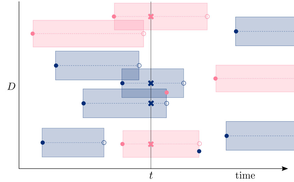 Figure 1
| Domain of interaction of particles. A metric space | |
| The set of types of particles, reds and blues | |
| , | Opposite color |
| Radon measure on | |
| Counting measure on | |
| The parameter of the exponential random variables describing patience of particles. | |
| Space of simple Radon counting measures on , with marks in | |
| Space of simple locally-finite ordered subsets of , with marks in | |
| , | Number of elements in |
| The set ordered as in | |
| , | Position, birth time, color and patience of , i.e., . |
| , | . |
| Region of maximum priority of . | |
| Ordered collection of particles present in the system at time | |
| Poisson arrival process used in the construction of the process. It is a random element of | |
| Set of discrepancies in the CFTP construction | |
| Killing function | |
| Matching function | |
| , | Marks to indicate whether a particle is matched or unmatched in the detailed processes |
| Backward detailed process | |
| Forward detailed process | |
| For , it is the number of unmatched particles among the first particles of . | |
| For , it is the number of matched particles excluding the first particles of . | |
| Density of the stationary measure of the Backward detailed process | |
| Density of the stationary measure of the process | |
| Janossy density of stationary version of the point process | |
| Set of all permutations of the elements of a finite set . | |
| The set of all paths in a square lattice from to | |
| A representation of the map that gives the canonical bijection between and . |
Peer Reviews
No public reviews on file for this paper yet. If you reviewed it on a platform where reviews are public (OpenReview, ICLR, NeurIPS, ICML), you can paste yours below so the community can read it here.
Videos
No videos yet. Explain this paper in a talk, walkthrough, or lecture? Add one.
On Spatial Matchings: The First-in-First-Match Case
Mayank Manjrekar
Abstract.
In this paper, we describe a process where two types of particles, marked by the colors red and blue, arrive in a domain at a constant rate and are to be matched to each other according to the following scheme. At the time of arrival of a particle, if there are particles of opposite color in the system within a distance one from the new particle, then, among these particles, it matches to the one that had arrived the earliest. In this case, both the matched particles are removed from the system. Otherwise, if there are no particles within a distance one at the time of the arrival, the particle gets added to the systems and stays there until it matches with another point later. Additionally, a particle may depart from the system on its own at a constant rate, , due to a loss of patience. We study this process both when is a compact metric space and when it is a Euclidean domain, , .
When is compact, we give a product form characterization of the steady state probability distribution of the process. We also prove an FKG type inequality, which establishes certain clustering properties of the red and the blue particles in the steady state. When is the whole Euclidean space, we use the time-ergodicity of the construction scheme to prove the existence of a stationary regime.
UT Austin, USA. E-mail: [email protected]
This work is supported by award from the Simons Foundation (award number 197982) to the University of Texas at Austin.
1. Introduction
Let be a metric space, with complete metric , and let be a Radon measure defined over it. Suppose for now that is compact, so that . We study the time-evolution of a continuous time stochastic Markov jump process whose state is defined by an ordered configuration of two types of points in . The two types are assigned to be the colors red and blue, and referred in short by the letters and respectively. A configuration here refers to a locally finite collection of points. When is compact, a configuration consists of finite number of points.
The process evolves over the space of ordered configurations on as follows. New particles of each type arrive according to an independent Poisson point process on with intensity , where is the Lebesgue measure on . Suppose, for instance, that a red particle arrives at time , at location . Then we look for the first blue particle in the ordered sequence whose distance to location is less than . If there is such a particle, , the new state is obtained by removing the particle from , while keeping the order of the remaining elements fixed. If there is no such particle, then the new state is obtained by adding a particle, with location and mark , to . In this case, the order within the elements of is preserved and the new particle is placed at the end of the sequence . The arrival of a blue particle is handled similarly. Additionally, any particle in the configuration is removed at a constant rate , while preserving the order of the remaining particles. Note that if is the empty configuration, then the ordering of particles in is simply the order in which those particles have arrived in the system. We will call this the First-in-first-match (FIFM) spatial matching process.
Figure 1 gives an illustration for the above dynamics.
1.1. Motivation and previous work
The motivation for studying this problem comes from modern shared-economy markets, where individuals engage in monetized exchange of goods that are privately owned in a via peer-to-peer marketplace. Examples of such marketplaces include ride-sharing networks, such as Uber or Lyft, and renewable energy networks with distributed generation of power. Here, consumers and producers can be viewed as individuals distributed in an abstract space, who engage in a transaction with others in close proximity. The abstract space could model factors such as location, product preferences, price and willingness to pay, etc. In the example of ride-sharing network, the position of an individual would correspond to its physical location, while in a renewable energy network, the position could model a combination of physical location and price. In this study, our goal is to comment on the spatial distribution of individuals in the long-run, under a well-defined matching scheme such as the one described in the introduction.
The underlying dynamics in our model can be viewed from a queuing theoretic viewpoint. Most queuing theoretic models study systems where there is an inherent asymmetry between customers and servers. Customers are usually transient agents that arrive with some load, and depart on being processed. Servers meanwhile are present during the whole life-time of the study of the stochastic process, and serve the customers according to a given policy. In the literature, there are only a few examples of queuing systems where customers and servers are treated as symmetric agents that serve each other. The double-ended queuing model discussed in [14] studies a model for a taxi-stop where taxis and customers arrive independently according to two Poisson arrivals. If a taxi (or a customer) arrives at the taxi-stop and finds a waiting customer (taxi) waiting, then it matches instantly, using say a first-come-first-serve (FCFS) policy, and both agents depart. Otherwise, the taxi (customer) waits until it is matched with a customer (taxi) that arrives later.
The FCFS bipartite matching model that was introduced in [7], and later studied in some generality in [1], is another such model. In this model, the customers and servers belong to finite sets of types, and respectively, which determine whom they can be matched to. The compatibility of matches between the various types of customers and servers is expressed in terms of a bipartite graph , where . The process, , is the ordered list of unmatched customers and servers arriving before time . At each time , one customer, , and one server, , arrive to the system. Here, and are independent sequences of i.i.d. random elements of and , with distributions and , respectively. is obtained from , and by matching and from elements in , if possible, using the FCFS policy, and removing the matched pairs. This model is called the FCFS bipartite matching model. In this series of works ([7, 2, 1]), the authors derive a product form distribution for the steady state under the so-called complete resource pooling condition:
[TABLE]
or equivalently,
[TABLE]
The authors also provide expressions for performance measures in the steady state, such as the matching rates between certain type of pairs, and waiting times of agents. These expressions are computationally hard to evaluate, owing to the hardness in computing the normalizing constant in the product form distribution.
We now briefly discuss variants of the FCFS bipartite matching model. Bušić et.al ([6]) generalize the bipartite matching model by dropping independence of arriving types and considering other matching policies. Büke and Chen [5] study a model where the matching policy is probabilistic. In their model, when a customer (server) arrives in a system, it looks at the possible matches and independently of everything else, selects one using a probability distribution. There is also a positive probability of not finding any suitable server (customer), in which case it starts to wait for a compatible server (customer). They also consider models where the users are impatient and may depart if they are not matched by a certain time. An exact analysis of these models becomes quite intractable and in [5] the authors study the fluid and diffusive scaling approximations of these systems.
The model we consider in this paper is essentially a continuous time and continuous space version of the model studied in [1], with the added feature that particles may also depart on their own due to a loss of patience. This spatial matching model is related to the FCFS bipartite matching model in the following sense. Just like the classes of customers and servers in that model, in our model, we still have two classes, the red and blue particles; each particle has a location in which is akin to the types within a class; and two particles are supposed to be compatible in the sense of the FCFS bipartite matching model, if they are within a distance one from each other.
In this paper, in the case when is compact, we derive a product form characterization of the steady state distribution of the process we consider. The analysis needed to obtain this product form distribution is an extension of the analysis in [1] to the continuum. We guess the reversed process and the steady state, and then check the local balance conditions to get the product form distribution in Theorem 2.3.
The two particle Widom-Rowlinson (WR) model is related to the distribution of the unordered configuration, , in the steady state of our model. The one and the two particle WR models were defined in [19] as a mathematical model for the study of liquid-vapor phase transition in physical systems. The two particle WR model is a point process that consists of two types of particles, and , as in the steady state of our process. This model on a compact domain can be described as the union of two Poisson point processes with intensities and , conditioned on the event that there are no two particles of opposite types within a distance one from each other. On the infinite Euclidean domain, , it is defined as a Markov random field (see [18]), with Papangelou conditional intensity and , where and are the collection of red and blue points of . The single particle WR model is obtained by marginalizing over one of the particles in the two particle WR model. The two particle WR model is interesting as it is the first continuum Markov random process where a phase transition has been rigorously established. It was basically established that, in the phase diagram, along the line , symmetry is broken when is large enough. This was first shown in [17] using an adaptation of Peierl‘s argument. [8, 12] independently give modern self-contained proofs of this phenomenon using percolation based arguments. The key ingredient in the proof in [8] is the observation that when we disregard the types of the particles, the resulting model, called the Gray WR model, is the continuum version of the random cluster model. The Gray model, in particular, satisfies the FKG property (with the usual lattice structure) and the corresponding positive association inequalities, that are crucial in showing existence of a percolation thresholds, and consequently a phase transition in this model.
Contrary to the two particle WR model, we believe that in our model, the unordered collection of the points in the steady state is not a Markov points process. The definition of a Markov point process (see Chapter 2 of [18]) requires, first, that there exists a symmetric reflexive relation over the domain, and second, that the Papangelou conditional intensity at a point depend on the configuration only through the points in that are related to the by . In our case, we are unable to show the existence of such a symmetric relation. However, we are able to show that the Papangelou conditional intensity at a point depends on the clusters of overlapping unit balls that intersect with the unit ball around the point.
In spite of this limitation, we show that the point process satisfies an FKG lattice property, with a specific lattice structure, similar to one satisfied by the two particle WR model (see Section 2 of [8]). The lattice structure as follows: we say if and only if and . The resulting positive association inequality can be used in conjunction with the results in [4], to prove that the points of the same type are weakly-super Poissonian. This is interesting since any exact analysis of the clustering of the steady state from its product form distribution is prohibitively hard as there is no closed form expression for its normalizing constant. In fact, in discrete systems, it is a -complete problem to compute the normalizing constant ([2]).
In this paper, we also consider the same matching dynamics in the infinite Euclidean domain . In this regime, using coupling from the past based arguments, we give a formal definition and a construction of the process, and show that there exists a stationary regime for this process. The existence of the stationary regime is obtained using certain coupling from the past ideas that were developed in [3].
In the following sections, we will discuss the notation required to formally define our model. Other notation will be required as we go along – see Appendix G for a table of notation. We begin Section 2 with the formal definition of the model in a compact domain. In Section 2.1, we give a coupling based argument that the steady state exists and is unique, and in Section 2.2, we present the product form distribution for this steady state. Then, in Section 2.3, we introduce and prove the FKG lattice property satisfied by the unordered version product form distribution. We then proceed to study the model in the infinite Euclidean domain, in Section 3. In Section 3.1, we give a construction and in Section 3.3, we give the construction of the stationary regime.
1.2. Notation
Let be any metric space, endowed with a Radon measure, . We use to denote the space of simple counting measures on . There is one-to-one correspondence between and the space of locally finite collection of points in . is equipped with the -algebra generated by the maps , , where is the Borel -algebra on . In our presentation, we will frequently abuse notation and use the same variable to denote both an element of and its support, which is a subset of .
Every particle in our model also carries information about its patience. To encode this, we need the notion of a marked counting measure. A marked simple counting measure on , with marks in a space , is a locally finite simple counting measure on such that its projection is an element of . We denote the space of all such measures by .
We will also require the definition of the space of locally-finite totally-ordered collection of points in the space , . For any , the order within the elements of will be denoted by . The order will be used to indicate the priority of the particles when matching with other particles. So, if the state of the system is and an incoming point is compatible with both , then it prefers over . has a natural projection onto , obtained by dropping the order within its elements – for any , the unordered collection is denoted by . For compact , may be canonically identified with . Finally, the space of totally-ordered marked locally-finite collection of points, with marks in , will be denoted by .
For any (or ), we will use the notation to denote the number of elements in , i.e., .
As mentioned in the introduction, the symbols and will be used to denote the types red and blue respectively. Moreover, we will let , and let a line over a color denote the opposite color, i.e., and .
2. First-in-First-Match Matching Process on Compact Domains
In this section, we first give a formal definition of the process on a compact domain. Let be a compact metric space with a Radon measure . The state of the process will contain information about the location, color and the order of arrival of the particles present in the system. Thus, the state space will be the set of totally-ordered collection of particles, with location in and with marks in the set , namely . The order represents the order of arrival of particles into the system, and hence represents their priority when two particles are in contention to be matched to the same particle.
We will require the following notation to describe the evolution of the process. For a point , we denote the projection onto by and denote the projection onto by . For any point , we denote the set of incompatible points of opposite color by , where denotes the ball of radius centered at . For any subset , we set . Let , where is the counting measure on . For any and , let be the element of formed by ordered as in . Further, if is represented as a list , then for any , , we set . The region of highest priority of a particle in , denoted (or just if the context is clear), is defined to be the set .
Let us recall the description of the dynamics in terms of the above notation. We consider a Markov jump process, . Suppose that a new particle, , arrives at time . If the ordered collection is non-empty, then the particle matches to the lowest-ranked particle in this set and the matched particle is removed from . Equivalently, matches to if and only if . Otherwise, is added to the ordered set at the end, so that for all , while the order among the elements of is preserved. Additionally, independent of everything else, particles may depart on their own when they lose patience at rate .
This description fixes the form of the generator of the process, which is given by
[TABLE]
where is a measurable function defined over . In the following we give an explicit construction of a process which will serve as the formal definition of our process. It can be easily verified that, if is the constructed process, then
[TABLE]
for any bounded continuous function over (we refrain from identifying the full domain of the generator). For us, the form of the generator will be useful in characterizing the stationary distribution, while the explicit construction will be useful later in the construction of the process on .
Let be a Poisson point process on , with i.i.d. marks in . The intensity of the point process is , where is the Lebesgue measure on . Both the marks are independent, with the color uniformly distributed and the other mark is an exponential random variable with parameter . Let be the initial state of the system at time [math]. Each point in is represented by four coordinates , with , and . denotes the spatial position of the point , denotes the time of its arrival, denotes its color and denotes its patience. The following display presents an algorithm for the construction of the process on compact domains.
•
Data:
a.
: A realization of the arrivals.
b.
: A realization of the initial condition.
c.
: End time of simulation.
•
Result: : The final state of the system as time .
(1)
Set .
(2)
For each , assign i.i.d. marks , that are exponentially distributed with parameter .
(3)
Set . If , quit and return .
(4)
If is due to arrival of a new particle (first infimum):
•
Let the particle be .
•
If there is a particle of opposite color in :
–
Match to the first particle of opposite color in and remove that particle. This gives .
•
Else:
–
Add the particle to the end of to give
(5)
Else if is due to a particle losing patience (second infimum), then remove this particle to yield .
(6)
Set . Go to Step 3.
2.1. Existence and Uniqueness of a Stationary Regime
In this section, we look at the stationary regime of the process on a compact domain , defined in Section 2. We first show that there is a unique stationary measure for this process, and in the subsequent sections give a product form characterization.
It can be seen that if in the model, we have , the process does not have a stationary regime. Indeed, in this case, starting from , . The process on the right-hand side does not have a stationary regime. So, we need to assume . It is easy to argue then, using a standard coupling from the past or a Lyapunov technique, that there is a unique stationary distribution. For the sake of completeness, we give a coupling from the past construction of a stationary regime and prove that it is unique.
Suppose we have a bi-infinite time-ergodic Poisson point process on , with marks in , where the first coordinate is the color of the particle and the second coordinate is the time the particle is the patience, as in the construction in Section 2. We define the notion of a regeneration time of the Poisson point process as follows. A time is called a regeneration time if for all , with , we have . That is, there is no possibility that a particle arriving before survives beyond time . For any process, , started with empty initial conditions at time , and driven by the process , we note that , for all and all regeneration times . Therefore, a stationary regime exists if we can show the existence of a sequence of regeneration times that diverge to almost surely. This is an instance of a coupling from the past scheme. The following lemma provides such a sequence of regeneration times.
Lemma 2.1**.**
Under the setting of this section, there are infinitely many regeneration times in the list , almost surely.
Proof.
Let us find the probability of the event, , that [math] is a regeneration time. We have:
[TABLE]
where in the third equation we have used the Fatou‘s lemma and the Laplace transform formula for Poisson point processes. Now, let be event that is a regeneration time. If is a time-shift operator, we have . By time-ergodicity of , must occur infinitely often, almost surely. Thus, there are infinitely many regeneration times in the list . ∎
The uniqueness of a stationary regime can also be show using a coupling argument. We only give an outline of this procedure here. Suppose we consider two stationary measures of the process. Let and be realizations of these two states. For large enough , the probability that and is less than . Conditioned on this event we may couple the processes in a time , using the coupling scheme from the previous lemma. Note that with such a scheme, we have . Thus, the total variation distance , using the coupling and the Markov inequalities. Since , we must have that must be equal in distribution to .
In the next section, we present a product form characterization of this steady state distribution. To do this, the key step is to construct the reversed process.
2.2. Product Form Characterization of the Steady State
Let be the driving Poisson point process on , with i.i.d marks in , that is given as data as defined in the coupling from the past construction in Section 2.1.
Lemma 2.1 implies that there exists a unique bi-infinite spatial matching process that is driven by . We can thus define a (random) matching function, , such that
[TABLE]
Conversely, stores all the information necessary to build the process . Indeed, the state of the spatial matching process we are interested in is given by
[TABLE]
where the list is ordered according to the birth-times, .
To get a handle on the stationary distribution of this process, we shall create its reversed process. Taking inspiration from [1], we will include some additional data in the state of the system that will simplify the description of the reversed process. We shall consider a process that we call the backward detailed process generated by and . This process contains unmatched and matched particles in its state, and we distinguish these types by using marks ’’‘‘ or ’’‘‘ respectively. For any particle in the state, will refer to this mark.
For , let
[TABLE]
be the time of arrival of the earliest among the unmatched particles at time . Let
[TABLE]
be the set of (location, arrival-times and colors of) unmatched particles in . Let
[TABLE]
be the set of so-called matched and exchanged particles that are present in . In the last expression, the first set of elements corresponds to particles that arrive in the relevant interval, , and are matched by the time ; but instead of recording their positions and types, we record that of their matches. The second set of elements in that expression corresponds to particles arrive before , that depart on their own in the time interval ; we record the time at which they depart.
Finally, define the backward detailed process, , be the list , ordered according to the values of . Clearly, the original process can be obtained from by removing the particles with marks . Notice that if , the first element in , denoted by , always satisfies .
The backward detailed process, , is a stationary version of a Markov process. A valid state of this Markov process is any finite list of elements, from the set that satisfies the following definition.
Definition 2.2** **(Definition of a valid state of
).
We say that a finite list of elements , with and , is a valid state of if the following three conditions are satisfied:
- (1)
, if . 2. (2)
For all , and implies that . 3. (3)
For all , , and implies that .
Condition 2 in the above definition essentially states that there cannot be a compatible unmatched pair in a valid state. This condition is equivalent to the condition that
[TABLE]
Condition 3 cannot be violated, since otherwise the particle whose matched and exchanged pair is could instead have matched to that arrives earlier. This condition is equivalent to the condition that for all ,
[TABLE]
Any valid state can be achieved by the process in finite time with positive probability. Indeed, starting from the empty state, a valid state, , can result from empty state if the arrivals occur in the order listed in , with appropriate patience so that the particles in marked survive until time , and the particles in marked exit on their own before the next arrival.
Transitions for occur at the time of arrival of a new particle or at the event of a voluntary departure. At the time of a new arrival, we match and exchange the particles in the list , and at the time of a departure, we put the departing particle at the end of the list , while updating the mark to . Below, we describe the transitions and transition rates of this Markov process in detail.
The transitions and transition rates for are as follows: Let , , be a valid state.
- (1)
A particle , with , loses patience: This occurs at rate . In this case, the new state is obtained by removing the and inserting at the end of the list . Additionally, we need to prune leading matched and exchanged particles from to obtain the new state. 2. (2)
A new particle arrives and is matched to a particle , with and : This occurs at rate . The new state is obtained by matching and exchanging the appropriate pair, and then pruning the leading matched and exchanged particles. 3. (3)
A new particle arrives and there is no particle of opposite color within a distance from it: This occurs at rate . The new state is the one obtained by adding this new particle to the end of the list as an unmatched particle.
We now guess the time-reversed version of the backward-detailed process, and obtain its transition rates. The following construction will be useful in doing this. Consider a dual process , that we call the forward detailed process. It is defined as follows: for let
[TABLE]
be the latest time at which all unmatched particles at time are matched or exit. Let
[TABLE]
be the matched and exchanged particles corresponding to the particles that are born before time , but have not been removed from the system by time . Let
[TABLE]
be the particles in the relavant interval , whose match arrives after time . Now, let , ordered according to the values . Thus, the last element in the list , always has . For motivations for these definitions, see [1].
Under our construction, using the bi-infinite Poisson point process , the process is a stationary process. In fact, it is a stationary version of a Markov process, since all the arrivals and deaths are Markovian. The transitions and transition rates are defined in detail in Appendix D.
The underlying idea in obtaining the product form distribution is the following. For any list of elements , let be the list of elements in written in the reverse order, with the marks and flipped. Then we claim that, a version of time-reversal of the backward-detailed process , is given by . That is,
[TABLE]
Indeed, the two processes are exactly equal if is constructed using the time-reversal of . We refrain from showing this observation in detail, and instead check the local balance conditions to obtain the product form result. See Appendix A for definition of local balance conditions.
Before we state the main result of this section, we need to fix some notation. For any list and , we define the to be the number of unmatched particles among the first particles on , and define to be the number of matched particles excluding the first particles of . In this notation, we may drop the reference to when the context is clear. Also, for the sake of brevity, we will write, for any , . We have the following result.
Theorem 2.3**.**
The density of the stationary measure of the backward detailed process, , w.r.t. the measure on , is given by
[TABLE]
where , and where is the normalizing constant,
[TABLE]
The proof of the above theorem is given in Appendix D.
For the stationary distribution of the original process , we compute the marginals of . Firstly, a state is a valid state of the process, , if and only if .
Corollary 2.4**.**
The density of the stationary distribution of the process , w.r.t. the on , is given by
[TABLE]
where is the same normalizing constant as in Theorem 2.3
Proof.
We calculate the marginal distribution of the unmatched particles from the distribution in 2.3. Given that is in the steady state, let , , denote the number of matched particles present between and in the detailed version of the process. The only restriction that these particles must satisfy is that they must be incompatible with . Integrating over the positions of each of the particles gives a factor . Thus, we have:
[TABLE]
∎
2.3. Clustering Properties and the FKG Property
In this section, we focus on the stochastic geometric properties of the steady state arrangement of the particles in space . Hence, we forget the reference to the order of the particles in the steady state. The Janossy density ([9]) of a point process intuitively is the relative probability of observing a given configuration of points with respect to a given reference measure. The Janossy density of the steady state distribution of our point process model, with respect to the Poisson point process on with intensity is given by dropping the order of particles in Equation 4. That is, the Janossy density is
[TABLE]
where is the set of all permutations of , and is a normalizing constant.
Let us take a moment to interpret the term that appears in the above expression. This is the sum of the volumes of the union of balls around red particles in and the union of balls around the blue particles in . Since such terms appear in the denominator in eq. 6, we expect that in the steady state the particles of the same color are clumped together.
In a variety of point processes, such as the one-particle Widom-Rowlinson model, or certain Cox processes [4], the FKG lattice property is a useful tool for proving stochastic dominance and clustering properties. In the case of Widom-Rowlinson model, the FKG inequality is also useful in showing the existence of a phase-transition [8]. The FKG lattice property defined on a measure over a finite distributive lattice states that for every ,
[TABLE]
If satisfies eq. 7, it is said to be log-submodular. The FKG lattice property implies the positive association inequality:
[TABLE]
for all increasing functions and on , where represents the expectation of with respect to .
This theorem can also be extended to point processes in the continuum as follows (see [11, 8] for details). Let is point process on a measurable space , with Janossy density with respect to a Poisson point process with intensity , the FKG lattice property states that:
[TABLE]
Under this hypothesis, one can conclude positive association inequalities such as eq. 8, where and are now increasing functions on .
Remark 2.5**.**
The FKG lattice property in the continuum point process case can also be stated in terms of the Papangelou conditional intensities: If is the Papangelou conditional intensity of a point process with Janossy density , then eq. 9 is equivalent to for all and with (see [11] for details).
In the following, we prove an FKG lattice property in the steady state version of our model, under a specific lattice structure defined on . Let and be two configurations in , where and are the red particles, and and are the blue particles in these configurations. We say that if and only if and . We note that the FKG lattice property is satisfied in the binary particle Widom-Rowlinson model with the same lattice structure. In [8], the authors also use discretization based arguments to lift the positive associations result for this lattice structure in the continuum.
To prove the FKG lattice property in our setting, we need the following auxiliary lemma.
Lemma 2.6**.**
Let and be two sets of positive numbers. Let be the set of all increasing paths in the grid , so that for any , we have , , and is either or , for all . Then, we have
[TABLE]
Here, and denote the and coordinate respectively.
The proof is by induction on . The proof is not central to the current discussion, so we present it in Section E.
We are now ready to prove a weak form of FKG lattice property for the Janossy density given in eq. 6.
Theorem 2.7**.**
Let and be disjoint finite subsets of such that the set is valid. Then, we have
[TABLE]
Moreover, if and are such that , then equality holds.
Proof.
Let and . There is a canonical bijection between and . For we denote by the corresponding element in . We will use the coordinate-wise notation for . Also, for any sets , let .
We have
[TABLE]
where in the second step we have used that
[TABLE]
and in the last step we used Lemma 2.6 with and . The proof now follows, since . Note also that if , then equality holds in eq. 11. ∎
The above theorem is useful in the proof of the main result of this section only through the following corollary.
Corollary 2.8**.**
If is a valid configuration (i.e., ), where and are the red and blue particles respectively in . Then,
[TABLE]
or equivalently,
[TABLE]
We now state the FKG lattice property for the usual subset ordering for the same type of particles.
Theorem 2.9**.**
Let and be finite subsets of . Then,
[TABLE]
A similar property holds when and are finite subsets of .
The statement of the previous theorem is combinatorial in nature. However, its proof is interesting since we were able to use probabilistic tools by introducing artificial randomness. In particular, at one stage in the proof, we employ the FKG inequality on the lattice (for some ). For the sake of exposition, this proof is moved to Appendix F.
Using Corollary 2.8 and Theorem 2.9, we conclude the main result of this section.
Corollary 2.10**.**
For any two finite subsets, and of , we have
[TABLE]
where the and .
Proof.
By Corollary 2.8 we have
[TABLE]
By Theorem 2.9, we have
[TABLE]
Now, since and are valid configurations, the proof follows by using Corollary 2.8 again. ∎
From Corollary 2.10 and the FKG inequality (see Appendix in [8]), we can conclude that the stationary measure is positively associated, i.e., for any two increasing functions and , then
[TABLE]
where is a version of the unordered stationary process, and has the density with respect to the Poisson point process with intensity . The above positive association inequalities also imply that the marginal point processes of the red (or the blue points) are also positively associated. This can be seen by taking increasing functions and that depend only on the red points (or the blue points). From this result and Corollary 3.1 of [4], we can conclude that and are weakly-super Poissonian. Intuitively, this means that the points are more clustered than the points in a Poisson point process of the same intensity.
2.4. Boundary Conditions and Monotonicity
In this section, we assume that is a compact subset of the Euclidean domain , for some . We will use the FKG lattice property to prove monotonicity of measures under different boundary conditions. To state these theorems we will require the following notation. Let be a valid state, i.e., . For any such boundary condition, we define a measure on with Janossy density
[TABLE]
Three important boundary conditions are , and . These are termed the red, the free and the blue boundary conditions respectively. We use special notation for the densities with these boundary conditions, namely, , and .
The boundary conditions can also be partially ordered: let if and only if and . We are now in a position to state the first result of this section.
Theorem 2.11**.**
Let be compact set. Let be two boundary conditions on . Then, the measure with density stochastically dominates the measure with density .
Outline of the proof.
By Holley‘s inequality [13], it is enough to prove that for two states, and , we have
[TABLE]
We first note that if and , then
[TABLE]
Since the red and blue subsets do not interact by Corollary 2.8, we only need to show that if and and , then
[TABLE]
The proof of the last statement follows by simple modification of the proof of Theorem 2.9, presented in Appendix F. Specifically, Equation LABEL:eq:fkg-4 in the appendix is modified to
[TABLE]
where the expectation is over a uniformly random choice
[TABLE]
The rest of the proof follows similar steps to the proof in Appendix F. ∎
Remark 2.12**.**
The above proof can be suitably modified to give the following interesting result. Let be two compact subsets of . With an abuse of notation, let denote the marginal-Janossy density of observing in , under the measure with density . Similarly, we overload the notation for . With this notation, we may prove that and . For the proof, we apply Holley‘s inequality, which requires that the following inequality holds:
[TABLE]
where are two valid configurations. This is follows from the inequality
[TABLE]
where is any configuration such that is a valid configuration. The later inequality can be proved using similar ideas used in the proof of Theorem 2.9 in Appendix F. We skip the details of the cumbersome calculations here. We will only remark here that, such a monotonicity of measures allows us to consider the limiting extremal measures and , on the infinite Euclidean domain . In the next few sections, we will consider the First-in-first-match process on infinite Euclidean domains, and prove the existence of a stationary regime. We leave the job of exploring of the connection between the stationary measure so obtained and these limiting measures to future work.
3. First-in-First-Match Matching Process on Euclidean domains
In the following few sections, we extend the definition of the process previously given on a compact space to a non-compact space. We will specifically focus on the Euclidean space , for some . The following methodology can be extended to other non-compact spaces that satisfy certain additional assumptions, but we refrain from presenting these results in complete generality. When , there are infinitely many arrival and departure events that are triggered in any finite interval of time. So, the process cannot be constructed as a jump Markov process using the algorithm presented in Section 2.
The key to the definition and construction of the process on is the following viewpoint. Let us look understand this viewpoint the compact setting first, and see its relation to the algorithm given in Section 2. Let be a compact space. Let and be the driving Poisson point process and the initial condition, respectively, as defined in the Section 2. Here, each particle is of the form , where , and are the position, color and patience of the particle. Similarly, any point is of the form , where additionally denotes the arrival time in .
We will treat as an element of , where the points of are ordered according to their birth times, as in Section 2. We will also treat as an element of , by setting for all , while preserving the order in . Moreover, we also consider as an element of , where all the elements of are ranked less than the elements of , while preserving the order within these sets.
We define a function , which we call the killing function, that is created as the process is built by the algorithm in Section 2. We set according to the following exhaustive set of rules.
- (1)
If arrives after and matches with it, then . 2. (2)
If is accepted into the system, then . 3. (3)
If , then .
According to the description of the process, the function satisfies the following recursive property. For any ,
[TABLE]
where the minimum above is set equal to if the above set is empty. In words, the conditions in the definition of the above set select particles of opposite color that arrive before (or are ranked lower), are accepted when they arrive, whose patience does not run out before arrives, and are not matched to any particle arriving before .
The above recursive property can serve as a definition of the function , even in the non-compact case, if we can show that the recursive definition terminates almost surely. We note that we could compute the value of if we knew all values of on points in that are within a spatial distance from and that arrive before it. It is also enough to just know all the values of for point in within a spatial distance that arrive before . The following lemma provides the tool needed to claim the termination of the recursive definition.
Lemma 3.1**.**
Suppose be a Poisson point process of intensity , where is the Lebesgue measure on corresponding Euclidean spaces. Then, there is no infinite sequence such that and for all .
Proof.
Let be fixed. Consider the event , where , , is the event that the Random Geometric graph (see [16]) obtained by joining any two points in whose positions are within a distance from each other does not percolate. From Theorem 3.2 of [16], we know that for every if is small enough. Hence, for small enough . This precludes the presence of an infinite sequence such that and , for all . Indeed, if such a sequence exists then the limit exists and by density of in , this event belongs to the set . ∎
The above lemma ensures that we can obtain the value of for any by recursively applying the Equation 18. The process in turn can be defined by setting
[TABLE]
for all . On the unbounded domain , this will serve as the definition of the FIFM spatial matching process.
3.1. Construction of Stationary Regime on Euclidean domains
The simple coupling form the past argument presented in Section 2 does not hold in the case where , since we cannot find a sequence of regeneration times going to in this case. We can show however that a coupling from the past argument can still be performed locally in space. This is done by first showing that, for a compact subset of the domain , there exists time beyond which two simulations agree for all times beyond time (So, is not a stopping time). A key ingredient in proving the existence of is an analysis of the decay in first order moment measures of the discrepancies between the two point patterns in simulation. Using this analysis, we are also able to bound the moments of , which enables the application of ergodic theorems, as applied in the simple coupling from the past construction in Section 2. In the following sections, we present this coupling from the past argument in detail.
3.2. A Coupling of Two Processes
We will first obtain some results about a coupling of two different processes, and , starting from the two different initial conditions, but driven by the same driving process . Let and be the two valid initial conditions (). At any time , there are some particles that are present in both processes. These particles will be called Regular particles, and denoted by. Call those particles that are present in and absent in as Zombies, and those that are absent in and present in as Antizombies. We denote them by and respectively. Further, call particles in as Special particles, and denote them by .
We now prove that the density of the special particles decays exponentially to zero.
Theorem 3.2**.**
There exist constants , , for all , where is the intensity of the special points, .
Proof.
Let be compact. Define and , and . Also, let for any , denote the set . Now, we will compute the difference for small , by tracking the changes that may occur in the short time interval . Recall that we use the notation to denote the domain of influence of the particle , . Also, in the following we have on . The following possibilities may occur:
- •
A zombie in exits on its own by losing patience. The expected difference is
[TABLE]
- •
With probability , two or more particles arrive or depart in . The expected change in , given that this occurs, is .
- •
A zombie in matches with a particle arriving in , which is accepted in the process . This results in a difference of
[TABLE]
- •
A zombie in matches with a particle arriving in , which is accepted in the process . This new particle is an antizombie. The resulting change is
[TABLE]
- •
A zombie in matches with an arriving particle, which also matches with some particle in in the complementary process. This results in an expected change of
[TABLE]
- •
A zombie in matches with an arriving particle, which also matches with some anti-zombie in . This results in an expected change of
[TABLE]
- •
An anti-zombie matches with a particle arriving in , that is accepted in the complementary process. This particle becomes a zombie. This results in an expected change of
[TABLE]
- •
An arriving particle matches with a zombie in and a regular particle in . The regular particle turns into a zombie. This results in a change of
[TABLE]
Hence, we have:
[TABLE]
Taking only the 2nd, 5th and 6th terms of the square braces of the above expression, dividing by , and taking the limit as , we obtain:
[TABLE]
We have similar bounds for derivatives of . Adding these expressions we obtain:
[TABLE]
Taking the limit , by spatial ergodicity of the process , we obtain
[TABLE]
from which we can conclude that . ∎
3.3. The Coupling from the Past Construction
In this section, we present the coupling from the past construction of the stationary regime. Let be a doubly infinite Poisson point process, as in Lemma 2.1. That is, is a Poisson point process defined on , with i.i.d. marks in . The intensity of the point process is and the marks are independent of each other, with the color uniformly distributed in and the patience an exponential random variable. Let be a sequence of time-shift operators such that . Let , , be a sequence of processes starting at time with empty initial conditions and driven by arrivals from . We have .
The processes and are driven by the same Poisson point process beyond time [math]. Treating the particles in as the initial conditions, we have a coupling of and as in Section 3.2. The discrepancies on any bounded set goes to zero exponentially fast by Theorem 3.2. In the following lemma, we show that such an exponential rate of convergence is enough to show that the time after which discrepancies never appear in any compact region has finite expectation. For any compact , define
[TABLE]
and in the following, let denote the set of discrepancies, . Note that is not a stopping time in our setting, since, first, for all a.s. (there are always discrepancies somewhere in ) by spatial ergodicity, and second, once discrepancies vanish in , they can reappear due to interactions with the particles from outside of .
We have
Lemma 3.3**.**
For all compact , .
Proof.
We view , , as a birth-death process. Let , where and are simple counting processes. Since new special particles only result from interaction of arriving particles with existing special particles, the rate of increase in is bounded above by . Hence,
[TABLE]
Since total departures are less than total arrivals, . This in particular shows that and exist and are finite a.s. Thus, also exists and is finite a.s. By dominated convergence theorem, . Thus, by Theorem 3.2, , a.s. This shows that a.s.
Further, we have:
[TABLE]
∎
Now, let be defined as
[TABLE]
denotes the time at which executions of processes and coincide inside the set . We have
[TABLE]
That is,
[TABLE]
Therefore, the sequence is a stationary and ergodic sequence. By Birkhoff‘s point-wise ergodic theorem and by Lemma 3.3,
[TABLE]
Therefore the last term in the summation, goes to [math] as . From this we conclude that
[TABLE]
This result has the following implication. For every realization of , any compact set and , there exists a such that for all , . That is, the execution of all processes , , coincides at time on the compact set . Then, locally in the total variation sense, the following limit is well-defined a.s. on the same probability space:
[TABLE]
The process is compatible since
[TABLE]
Further, the process can also be shown to be compatible. Indeed, fix . Let us implement a similar coupling from the past procedure, but with processes that start with empty initial conditions at time , . If is the process obtained in such as manner, it can be shown that is equal to generated as above. Thus, . This proves the is the stationary regime of the process.
4. Conclusion and Future Work
In this paper, we focused on a dynamic matching model with a natural policy, under the added assumption that particles may depart without being matched. We were able to find a characterization of the steady state distribution of the particles. Then using this characterization, we proved the FKG lattice property, which in turn enabled us to conclude that the property that particles of the same type are weakly-super Poissonian. We also prove that there is a stationary regime for the dynamics is the infinite Euclidean domain, .
The two particle Widom-Rowlinson model is a simpler model, where the FKG property, as satisfied by our model, is also satisfied. There, this property is used to show the existence of Markov random fields on the infinite Euclidean domain, . In the future, we would like to see whether this construction works in our setting, and how it relates to the stationary regime constructed on the domain .
The gray version of two particle WR model, which is obtained by removing the reference to the colors of the points also satisfies an FKG inequality – we are unable to prove this in our setting. This is a fundamental step in the symmetry breaking argument of [8]. We have not found such an argument in our setting. A symmetry breaking argument will show, for certain values of the parameter, that there are more red points than blue points in the steady state, or vice-versa. This also has implications on the relaxation times of the Markov process on finite domains. In the future, we would like to explore these problems.
Appendix A Dynamic reversibility of Markov processes
In this section we give a brief discussion of a result needed to construct the product form distribution. This concept will be termed dynamic reversibility of a Markov process, following the terminology in [15], where the concept was discussed for Markov processes on countable state spaces. We thus define it on countable state spaces first, and then on general state spaces.
Let be a stationary, irreducible continuous-time Markov process with values in a countable state space . Let denote the transition rate from state to and let be the stationary distribution of the process. In this case, the balance equations are .
The reversed process, , is also a stationary Markov process with transition rates . The converse of this statement can be used as a characterization of the stationary distribution. We state this result in the following theorem.
Theorem A.1**.**
Let be a stationary irreducible Markov process with transition rates . If there exists a collection of numbers , and a probability measure on such that
[TABLE]
then is the stationary distribution of the process and is the transition rate matrix for the reversed process.
Thus, if we can guess the transition rates of the reversed process and a stationary measure, we can verify them by checking a local balance condition of the form eq. 31. See Theorem 1.13 of [15] for a proof of this result. In practice, finding is usually as intractable as finding the stationary distribution directly. However, occasionally we may come across pairs of Markov processes that are reversed versions of each other, perhaps after a transformation of the state space. We state this phenomenon in the next theorem.
Theorem A.2**.**
Let be two countable spaces. Let and be two stationary irreducible Markov processes with values in and , and transition matrices and respectively. Suppose there is an isomorphism between the two spaces. Also suppose that there is a probability measure on such that
[TABLE]
then is the stationary distribution of and is the stationary distribution of .
Theorem A.2 can be stated in a more general setting, which we now state and prove.
Theorem A.3**.**
Suppose and be two locally compact Hausdorff topological spaces. Let and be two stationary Markov jump processes with values in and . Suppose that probability semi-group of the process () is characterized by the generators (), that is defined over (), where the domain is a subset of the Banach space of continuous functions over () vanishing at infinity, equipped with the uniform norm topology. Let be a measure space isomorphism such that for all , we have . If is a probability measure on such that
[TABLE]
then is a stationary distribution for .
Proof.
Let be any element in . Taking a sequence such that converges pointwise to the constant function , as , we have
[TABLE]
By standard results from the theory of positive operator semi-groups it is known that for implies that the map belongs to (see Lemma 1.3 of [10] for example). Thus, for , we have
[TABLE]
It is also known that is dense on the space of continuous functions vanishing at infinity (Theorem 1.4 of [10]). This implies that for all bounded continuous functions and all , and so, must be a stationary measure of . ∎
If two processes satisfy the hypothesis of the above theorem, we say that the processes are dynamically reversible.
Appendix B Some Additional Global Notation
In the following few sections we need some useful universal notation to define the transitions in the Markov processes. We collect them here in this section.
Let , and respectively be a list of elements and a particular element belonging to the same abstract space . We define the following operators:
- (1)
Let , , denote the insertion of element after the -th element in , i.e.,
[TABLE] 2. (2)
Let , , denote the removal of the -th element of , i.e.,
[TABLE] 3. (3)
Let denote the replacement of the element in with , i.e.,
[TABLE] 4. (4)
In the above notation, we may drop the subscript if , i.e., when we are making changes to the last element.
Appendix C Continuous-Time FCFS Bipartite Matching Model with Reneging
In this section, we illustrate how dynamic reversibility is used in the proof of Theorem 2.3, by working on a countable state space Markov model. This allows us to organize and present the main ideas without the complexity of dealing with measure valued processes.
Specifically, in this section, we consider the following modified version of the First-come-first-serve bipartite matching model considered in [1]. Consider two finite sets of types and and a bipartite compatibility graph with . Let be a measure on , and be a parameter. We say that and can be matched together or are compatible if in the compatibility graph . We define the first-come-first-serve bipartite matching model with reneging as a Markov jump process with state space, , which is the set of all finite ordered lists of elements from such that for every and in the list, . Further, given that the state of the process at any time is , the state is updated with the following transition rates:
- (1)
A new element arrives at rate . At the time of the arrival, if there is one or more elements in that is compatible to , then the first such element, , is removed, and we say that and are matched. If there is no such element, then is added to the end of the list . 2. (2)
Each element in the list is removed at rate .
The comments and results of Sections 2.1 and 2.2 can be mirrored in this setting. We briefly review them here.
We can simulate the above process by using arrival from a Poisson point process on , with i.i.d. exponential marks in , and with intensity . The base of the Poisson point process encodes the arrivals of the agents, and the mark of a point encodes the time each agent is willing to wait (its patience), if they are accepted. We will use the following notation: for any point , will denote its projection onto , will denote the second coordinate, and will denote the third coordinate.
Standard coupling or Lyapunov based arguments can be used to show that this Markov process has a stationary regime. Moreover, a stationary version of the process can be constructed by using a coupling from the past scheme that uses an ergodic arrival process, , which is now a Poisson point process on , with marks as above. To construct the stationary regime, the notion of regeneration time of the system may be defined as follows. We say that is called a regeneration time of if for all with , we have . The forward-time construction of the process starting from a regeneration time with empty initial conditions is clear. Moreover, if are two regeneration times and and are such processes starting from and respectively, then for , . Thus, we can construct a bi-infinite stationary version, , of this process as a factor of , if we can find a sequence of regeneration times going to . Indeed, if is such a sequence (and set ), then the for , and for some , is obtained by simulating the process starting from empty initial conditions from time until time . An argument similar to the Lemma 2.1 can used to show the existence of such a sequence of regeneration times.
This coupling from the past scheme gives the definition of the matching function,
[TABLE]
similar to the one defined in Section 2.2. For , let , be a regeneration time before . The value of can be set by simulating the process using , starting from time , with empty initial conditions. If is matched to an agent , then . Otherwise, if reneges, then .
Given the function , we can obtain the process , since , where the agents in the list are ordered according to their birth-times . Let and be additional marks, referring to whether an agent is matched or unmatched respectively. Consider the following detailed stochastic process : for ,
- (1)
Let . 2. (2)
Let and . 3. (3)
Define , where refers to the matched or unmatched status of an agent , and the list is ordered according to their second coordinates, .
Clearly, can be obtained from by removing the agents with marks . We call the process the Backward detailed process, following the terminology in [1].
Since the backward detailed process at time only depends on the points of before time , it is a stationary process. Moreover, it is a stationary version of some Markov process since for , the state at time can be constructed using the state at time and the process in the interval . We describe this Markov process in detail now. A valid state of this Markov process can be a finite list of elements, from the set such that
- (1)
, if . 2. (2)
If then . 3. (3)
For all , if and then .
Below, we utilize the definitions in Section B. Additionally, mirroring our notation in the continuum setting, we define for any , let and for any let . With an abuse of notation, we will let for . Also, for and any , we will denote
- •
,
- •
and ,
- •
[TABLE]
The transitions and transition rates for the backward detailed process are the following: Given that the state of system is ,
- (1)
any agent , with , loses patience. In this case, the new state is , except possibly when , where we need to prune all the leading matched and exchanged elements from . We still denote the new state by , even in this case, keeping in mind the all leading matched terms must be removed. Each such transition occurs at rate . 2. (2)
a new agent , , arrives and is matched to the agent , with and . In this case, the new state is (a valid pruning of) . This occurs at rate . 3. (3)
a new agent , with arrives and is not matched to any agent. The new state is . This occurs at rate .
We now define the Forward detailed process, which is the dual of the process , that we denote by . For , define
- (1)
Let . 2. (2)
Define , and . 3. (3)
Define , where the elements are ordered according to the second coordinates .
The forward detailed process is also a stationary version of a Markov process. Any valid state, , of this Markov process of the system satisfies:
- (1)
, when . 2. (2)
If , then . 3. (3)
If , , , then .
The transitions and the transition rates of the Markov process are given as follows: Given that the state of the system is , the next jump occurs at rate , where is the number of matched elements in after -th location. Intuitively, this is so because the total rate of new arrivals is and the total death rate is , since is the number of unmatched agents in the forward process. For the sake of brevity, let us denote by , for all . If is non-empty, at each jump, to obtain the new state, we need to process the first element, , in . This is done with the following probabilities:
- (1)
If is matched, then it is removed from . The new state is . 2. (2)
If is unmatched, then for the next state, we sample a random variable with distribution
[TABLE]
and then sample i.i.d. random unmatched elements in with distribution .
- (a)
If there is a FCFS matching , , then set the new state to , with the understanding that all the ending unmatched agents are discarded. 2. (b)
If there is no FCFS matching, set the new state to .
If the state is , then the next jump occurs at rate . When a jump occurs, a random unmatched point is sampled with distribution . The next state is decided as in step (2) above, with this new , we ignore the details here.
We have the following theorem.
Theorem C.1**.**
The two processes and are dynamically reversible. The concerned isomorphism is the one that takes a valid state , reverses the order of its elements and flips the marks and . The stationary distribution is
[TABLE]
where and where is a normalizing constant.
Outline of the proof.
To prove this, we start by looking at the balance equations of the form in Theorem A.2. Let be the state of the backward detailed process, and let be a state after a valid transition. In the following, we illustrate the local balance condition eq. 31 for only one type of transition. Other kinds of transitions can be handled similarly. Let and be the transition rates of the backward and forward detailed processes respectively. Also, let denote the type of the -th element in for any .
Suppose that , , and that is obtained from when one of the elements at , at some location , is matched and exchanged with a new arrival . In this case, and
[TABLE]
The first elements in are and . Moreover, for . Hence, eq. 32 simplifies to
[TABLE]
We claim that local balance equations for other valid transitions can also be handled similarly. This completes the proof this theorem. ∎
Appendix D Proof of Theorem 2.3
In this section we present detailed calculations to show that the backward detailed process, , and the forward detailed process, , defined in Section 2.2, are dynamically reversible as jump Markov process. In turn, we are able to prove Theorem 2.3.
We first define the valid states of the Markov process corresponding to the forward detailed process, and present the transitions and the transition rates, since these were skipped in the discussion in Section 2.2.
A valid state of the forward detailed process is given by the following rules.
Definition D.1**.**
is a valid state of the forward detailed process if
- (1)
, if , 2. (2)
For all , if and , then , 3. (3)
For all , if , and , then .
Condition 2 in the above definition essentially states that there cannot be a compatible matched pair in a valid state. This condition is equivalent to the condition that
[TABLE]
This is because, if there was a violating pair at time , such a pair could have potentially matched to each other before time instead of matching to their present matches. Condition 3 is required since otherwise a violating pair and , , the particle could potentially have matched with the particle instead, which arrives before the particle is matched to. This condition is equivalent to the condition that for all ,
[TABLE]
The Markov process corresponding to evolves as follows. Let , , be the state of the system at some time . The next jump occurs at rate . If is non-empty, the first element, , in the list is processed at the next jump according to the following rules.
- (1)
If is matched, then it is removed from . The new state is . 2. (2)
If is unmatched, then for the next state, we sample a random variable with distribution
[TABLE]
and then sample i.i.d. random unmatched points in with distribution .
- (a)
If there is a first-in-first-match , , for , then set the new state to , with the understanding that all the unmatched particles at the end of the list are discarded. 2. (b)
If there is no FIFM matching, then set the new state to .
If the state is , then the next jump occurs at rate . A random unmatched particle is sampled from with distribution . The next state is decided as in step (2) above with .
We are now ready to prove Theorem 2.3.
Proof of Theorem 2.3.
To obtain the stationary distribution, we check the conditions of Theorem A.3. The space is viewed as a subset of , and we use the induced topology on . With this topology, is a locally compact Hausdorff space. Let and let be the measure on . The probability semi-group of the processes acts over the Banach space of continuous functions that vanish at infinity, where we use the uniform norm topology. Moreover, the generator of can at least be defined on the space of compactly supported continuous functions, and has the form:
[TABLE]
Similarly, it can also be seen that the generator of can also be defined over the space of compactly supported continuous functions, and the value of the generator is the sum of the following terms (in the order of the transitions listed earlier):
- •
(1): ,
- •
(2a):
[TABLE]
where we have set for all .
- •
(2b):
[TABLE]
where for all .
When , we have the following terms in .
- •
(2a.):
[TABLE]
where, for all .
- •
(2b.):
[TABLE]
where, for all .
For the product form distribution, we check the balance condition of Theorem A.3, with an appropriate measure space isomorphism . The isomorphism is given by the function , defined in Section 2.2, that reverses the order and flips marks and of a valid state. In the following, let denote this function.
Taking any two compactly supported continuous functions , and taking each term of , we show that it corresponds to a few terms in , so that the sum of these expressions is equal. In particular, the following steps suffice.
- (1)
Take the first summation term of when it is expanded using eq. 33. Take -th term, with . Set . Let , and so . Also, let and . The corresponding term is
[TABLE]
where in the second equality, we have used that , and in the third equality, we use
[TABLE]
Similarly, in the first summation term of , taking , and letting be the maximum element such that are all matched in , we have
[TABLE]
where we have used the fact that if , then . Consider the first term in the above expression. Setting and , we obtain:
[TABLE]
where are i.i.d. particles in with marks , with distribution . Using a similar computation as in eq. 35, it is easy to see that RHS of eq. 37 is
[TABLE]
Similarly, the second term in the eq. 36 is
[TABLE]
where, are as before, and is an independent sample from with mark . 2. (2)
Now, take the second summation in , and the -th term, , in that summation. Using a similar computation as in previous item, we obtain:
[TABLE]
Setting and , we have the RHS of the above equation is equal to
[TABLE]
Similarly, taking first term in the second summation, and letting as before, we have
[TABLE]
Computations similar to the one in eqs. 37 and 38 show that the above is equal to
[TABLE]
where and are i.i.d. with marks and are i.i.d with marks . 3. (3)
Finally,
[TABLE]
Setting , , we have
[TABLE]
Since summing over the RHS of equations LABEL:eq:test1 to LABEL:eq:test5, for all , we get , we conclude that the two Markov processes and are dynamically reversible with respect to . ∎
Appendix E Proof of Lemma 2.6
The proof is by induction on . For , we need to show that
[TABLE]
We use induction on to prove eq. 43. For , this is clear, since
[TABLE]
Let the length of the sequence be . Assuming the inductive hypothesis for eq. 43, we have
[TABLE]
where in the first step we have grouped the first terms together. This finishes the proof of the base case (eq. 43) for the induction on .
Now, suppose that the length of the sequence is equal to , . Let , , denote the set of paths in where the first jump is at location . We have the following decomposition of the summation
[TABLE]
where denotes the path obtained by inserting a jump in the -th location of . Thus,
[TABLE]
The inner-most summation in the above expression is the case of this lemma, and therefore, by the induction hypothesis, we get that the
[TABLE]
where is the sequence of length with , for . Therefore,
[TABLE]
by the induction hypothesis. This completes the proof the lemma.
Appendix F Proof of Theorem 2.9
Let , and . The statement of the theorem is equivalent to showing that
[TABLE]
Let denote another copy of the , where we add over-lines to the particles to distinguish them from particles of . Also, for any , let .
Using the auxiliary Lemma 2.6, the LHS of the inequality above can be expressed as
[TABLE]
where we use to represent the first and second coordinates of .
Since
[TABLE]
we claim that eq. 45 is greater than
[TABLE]
Let be the set of all increasing vertex paths from to in , and , for all . We denote the coordinates of by . Using the canonical bijection between
[TABLE]
we see that eq. 47 is equal to
[TABLE]
Applying similar reductions to the RHS of eq. 44, we note that the result follows if we prove
[TABLE]
Note that the only difference in the left and right sides of the last inequality are the terms and .
Equation LABEL:eq:fkg-toprove can be expressed in the following equivalent way
[TABLE]
where the expectation is over a uniformly random element of the set . In the following, we will simply write in place of the symbol .
To prove eq. LABEL:eq:fkg-4, we first prove it on a smaller -algebra. We say that two permutations and are equivalent if by dropping the overline marks of the particles in in both and , we obtain the same sequence of elements. Let denote the -algebra generated by this equivalence relation. We show that for any ,
[TABLE]
Fix . We can express as a composition of a permutation and , so that . Since all permutations in the equivalence class of are equally likely, each conditional expectation in eq. LABEL:eq:fkg-cond-ineq can be expressed as an expectation over auxilliary i.i.d. Bernoulli random variables . To make this precise, let , , and for all and . Also, let and similarly, . We have
[TABLE]
Using the fact that for any , we may write the above inequality as
[TABLE]
It is enough to prove that the integrand in positive for every . Symmetrizing the expression, by replacing with , we obtain the following equivalent expression.
[TABLE]
To prove this, we use the FKG inequality on the lattice with measure
[TABLE]
Claim F.1**.**
The measure is log-submodular.
Proof.
Let . Then,
[TABLE]
Let us look at the first term in eq. 55. We have
[TABLE]
which is non-positive since is contained in both and .
Similarly, we may prove that the second term in eq. 55 is non-positive. For the third term in that equation, we have:
[TABLE]
By symmetry,
[TABLE]
Therefore,
[TABLE]
Consequently, . ∎
Now we show that the two relevant functions in eq. 54 are increasing in .
Claim F.2**.**
The functions
[TABLE]
are increasing in .
Proof.
Let . For any , let . Using the inclusion-exclusion formula, we may write
[TABLE]
Now, let be given. Fix . Fixing all , and taking the difference of the values of when and , we obtain:
[TABLE]
since we have assumed that . Similarly, taking
[TABLE]
we have
[TABLE]
Thus, . By symmetry in the problem, this is also true for . ∎
We are now in a position to apply the FKG theorem to the RHS of eq. 54, and since
[TABLE]
we obtain the result.
Appendix G Table of Notation
Acknowledgements
The author would like to thank his PhD advisor, Prof. François Baccelli, for many valuable discussion on this problem.
The reference list from the paper itself. Each links out to its DOI / PubMed record.
- 1[1] I. Adan, A. Bušić, J. Mairesse, and G. Weiss. Reversibility and Further Properties of FCFS Infinite Bipartite Matching. Mathematics of Operations Research , 43(2):598–621, 5 2018.
- 2[2] I. Adan and G. Weiss. Exact fcfs matching rates for two infinite multitype sequences. Operations research , 60(2):475–489, 2012.
- 3[3] F. Baccelli, F. Mathieu, and I. Norros. Mutual service processes in euclidean spaces: existence and ergodicity. Queueing Systems , 86(1-2):95–140, 2017.
- 4[4] B. Błaszczyszyn and D. Yogeshwaran. On comparison of clustering properties of point processes. Advances in Applied Probability , 46(1):1–20, 2014.
- 5[5] B. Büke and H. Chen. Fluid and diffusion approximations of probabilistic matching systems. Queueing Systems , 86(1-2):1–33, 2017.
- 6[6] A. Bušić, V. Gupta, and J. Mairesse. Stability of the bipartite matching model. Advances in Applied Probability , 45(2):351–378, 2013.
- 7[7] R. Caldentey, E. H. Kaplan, and G. Weiss. Fcfs infinite bipartite matching of servers and customers. Advances in Applied Probability , 41(3):695–730, 2009.
- 8[8] J. Chayes, L. Chayes, and R. Kotecky. The analysis of the widom-rowlinson model by stochastic geometric methods. Communications in Mathematical Physics , 172(3):551–569, 1995.