A Comparison of Different Classical, Semiclassical and Quantum Treatments of Light-Matter Interactions: Understanding Energy Conservation
Tao E. Li, Hsing-Ta Chen, Joseph E. Subotnik

TL;DR
This paper compares classical, semiclassical, and quantum methods for simulating light-matter interactions, highlighting the accuracy of the Ehrenfest+R approach in energy conservation and correct optical signal prediction.
Contribution
It demonstrates that the Ehrenfest+R method accurately reproduces quantum optical signals and energy conservation, outperforming traditional approaches in semiclassical light-matter interaction simulations.
Findings
Ehrenfest dynamics are accurate only in the linear response regime.
Maxwell-Bloch and dielectric theory predict incorrect signals due to double-counting.
Ehrenfest+R approach correctly balances self-interaction and quantum fluctuations.
Abstract
The optical response of an electronic two-level system (TLS) coupled to an incident continuous wave (cw) electromagnetic (EM) field is simulated explicitly in one dimension by the following five approaches: (i) the coupled Maxwell-Bloch equations, (ii) the optical Bloch equation (OBE), (iii) Ehrenfest dynamics, (iv) the Ehrenfest+R approach and (v) classical dielectric theory (CDT). Our findings are as follows: (i) standard Ehrenfest dynamics predict the correct optical signals only in the linear response regime where vacuum fluctuations are not important; (ii) both the coupled Maxwell-Bloch equations and CDT predict incorrect features for the optical signals in the linear response regime due to a double-counting of self-interaction; (iii) by exactly balancing the effects of self-interaction versus the effects of quantum fluctuations (and insisting on energy conservation), the…
Click any figure to enlarge with its caption.
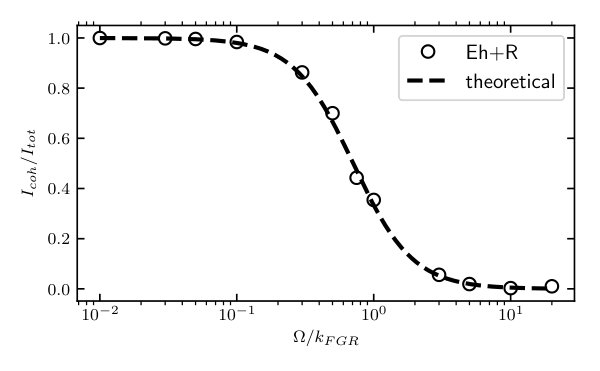 Figure 1
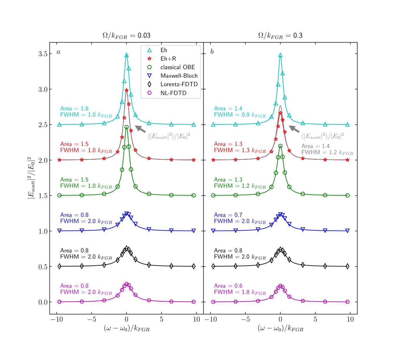 Figure 2
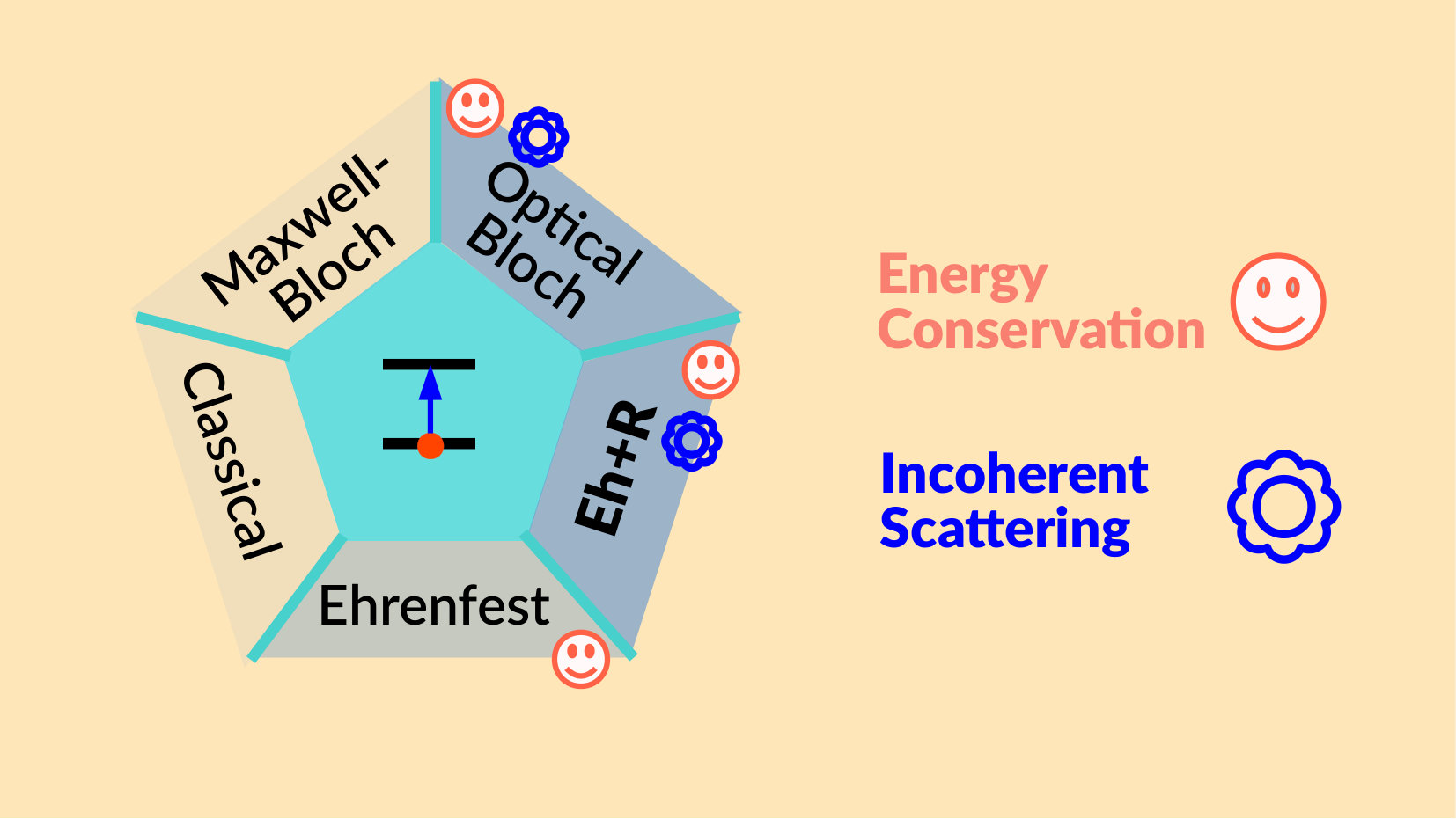 Figure 3
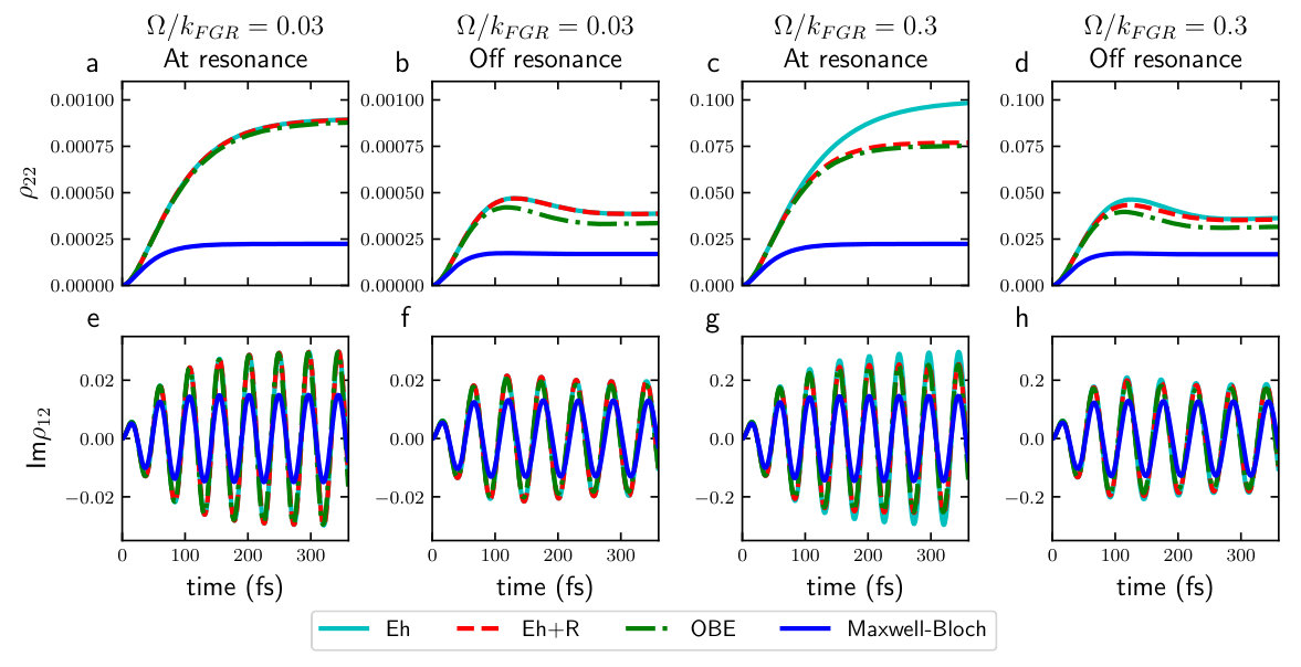 Figure 4
| Approach | Recover SE | Equation of motion for optical polarization | Energy conservation59 |
|---|---|---|---|
| Optical Bloch | True | True (QOBE) | |
| Eqs. (13) and (17) | / False (COBE) | ||
| Maxwell–Bloch | False | False | |
| Eqs. (12-16) | |||
| Ehrenfest | False (True only | True | |
| Eqs. (20) and (16) | when ) | ||
| Ehrenfest+R | True | True | |
| Appendix B | |||
| CDT-Lorentz | — | False | |
| Eqs. (29-31) |
Peer Reviews
No public reviews on file for this paper yet. If you reviewed it on a platform where reviews are public (OpenReview, ICLR, NeurIPS, ICML), you can paste yours below so the community can read it here.
Videos
No videos yet. Explain this paper in a talk, walkthrough, or lecture? Add one.
A Comparison of Different Classical, Semiclassical and Quantum Treatments of Light–Matter Interactions: Understanding Energy Conservation
Tao E. Li
Department of Chemistry, University of Pennsylvania, Philadelphia, Pennsylvania 19104, USA
Hsing-Ta Chen
Department of Chemistry, University of Pennsylvania, Philadelphia, Pennsylvania 19104, USA
Joseph E. Subotnik
Department of Chemistry, University of Pennsylvania, Philadelphia, Pennsylvania 19104, USA
Abstract
The optical response of an electronic two-level system (TLS) coupled to an incident continuous wave (cw) electromagnetic (EM) field is simulated explicitly in one dimension by the following five approaches: (i) the coupled Maxwell–Bloch equations, (ii) the optical Bloch equation (OBE), (iii) Ehrenfest dynamics, (iv) the Ehrenfest+R approach and (v) classical dielectric theory (CDT). Our findings are as follows: (i) standard Ehrenfest dynamics predict the correct optical signals only in the linear response regime where vacuum fluctuations are not important; (ii) both the coupled Maxwell–Bloch equations and CDT predict incorrect features for the optical signals in the linear response regime due to a double-counting of self-interaction; (iii) by exactly balancing the effects of self-interaction versus the effects of quantum fluctuations (and insisting on energy conservation), the Ehrenfest+R approach generates the correct optical signals in the linear regime and slightly beyond, yielding, e.g., the correct ratio between the coherent and incoherent scattering EM fields. As such, Ehrenfest+R dynamics agree with dynamics from the quantum OBE, but whereas the latter is easily applicable only for a single TLS in vacuum, the former should be applicable to large systems in environments with arbitrary dielectrics. Thus, this benchmark study suggests that the Ehrenfest+R approach may be very advantageous for simulating light–matter interactions semiclassically.
{tocentry}
1 Introduction
The nature of light–matter interactions is a never-ending source of stimulation in both experimental and theoretical science. To theoretically study light–matter interactions at the atomic and molecular level, non-relativistic quantum electrodynamics (QED)1 is the ultimate theory: the matter side obeys the Schrödinger equation (or the quantum Liouville equation) and the radiation field is quantized as photons. And for weak light–matter interactions, perturbative approximations of QED are both practical and adequate for describing most experimental findings. However, to understand recent experiments that involve strong light–matter interactions2, 3, 4, 5, 6, 7, one must go beyond the perturbative limit of QED. Furthermore, if we cannot use linear response theory, then both matter and photons must be simulated explicitly and on the same footing. Moreover, because photons are described in a vast infinite-dimensional Hilbert space, a rigorous QED treatment becomes a computational nightmare for calculations applicable to most modern work in nanoscience.
To reduce the computational cost of QED, one plausible simplification is to work in a truncated space of photons, i.e., to consider a subspace with either only a few photon modes or a few photon quanta per mode. In the framework of this simplification, one approach is to invoke Floquet theory8, 9; another approach is to construct a dressed state representation10. Both techniques can accurately describe strong light–matter interactions. Unfortunately, however, these techniques are usually applicable only when modeling either systems exposed to cw light or systems encapsulated in model three-dimensional (3D) cavities.
For large scale simulations of material systems in arbitrary EM fields and not necessarily in a full-3D cavity, a more promising ansatz would appear to be semiclassical electrodynamics11, 12, 13, according to which the matter side is described quantum-mechanically and the radiative electromagnetic (EM) fields are treated classically. More precisely, one replaces the EM field operators (acting in an infinite-dimensional Hilbert space) by c-numbers and propagates the dynamics of the EM field using the classical Maxwell’s equations. Compared with QED calculations, semiclassical approaches are computationally much more affordable, and one can still preserve more of the quantum nature of light–matter interactions than standard classical electrodynamics (where the matter side is described as a dielectric constant14). Thus, semiclassical electrodynamics would appear to be a natural compromise between speed and accuracy.
Now, although semiclassical approaches have many appealing qualities, one inevitable question arises: can one actually capture any true quantum effects of the EM field using such techniques? For example, because of the nature of the quantum radiation field, an electron in an excited state can automatically decay to its ground state even when no external field is applied, a phenomenon known as spontaneous emission. As has been argued by many (including Cohen-Tannoudji)15, 16, 17, 18, this spontaneous process can in fact be dissected into two well-defined sub-processes: (i) first, vacuum fluctuations that arise from the zero-point energy of the EM field; (ii) second, emission carried by electronic self-interaction as the scattered EM field induced by the electron reacts back on the electron itself. While the latter has a classical analog (e.g., the Abraham-Lorentz equation19, 20), the former is a purely quantum effect. Can spontaneous emission be captured by semiclassical approaches (i.e., Ehrenfest dynamics21, 22, 23)? In fact, it is well-known that, according to Ehrenfest dynamics (or neoclassical electrodynamics24), only self-interaction is taken into account in the equation of motion for the electron: vacuum fluctuations are not included. As a result, an electron is stabilized in the excited state according to Ehrenfest dynamics, thus violating many experimental observations of florescence. A lack of spontaneous emission is one failure of semiclassical electrodynamics theory, and one would like to go beyond Ehrenfest when simulating large systems where spontaneous emission cannot be ignored.
1.1 Beyond Ehrenfest dynamics
Perhaps the most straightforward way to correct Ehrenfest dynamics so as to include spontaneous emission is to add a linear, "hard" dissipative term on top of the Liouville equation for the matter side and thus force the electron to decay without concern for the dynamics of the EM fields. This approach makes sense since the overall spontaneous decay rate in vacuum (as carried by self-interaction plus vacuum fluctuations) is a constant — known as the Fermi’s golden rule (FGR) rate — regardless of the instantaneous electronic state. By further assuming that the external field influences the electron in a classical way and does not alter the spontaneous decay rate of the electron, one arrives at the coupled Maxwell–Bloch equations25, 26 for modeling light–matter interactions. According to a naïve implementation of the coupled Maxwell–Bloch equations, the EM field that one molecule feels is composed of both the incident externally imposed EM field plus the scattered field generated by the molecule itself. Given that Ehrenfest dynamics already incorporates self-interaction (as just discussed; see Refs. 22, 27), it is then perhaps not surprising that one can show that a naïve Maxwell–Bloch scheme actually double-counts the electronic self-interaction28.
To avoid such nonphysical double-counting, many additional efforts have been made to exclude the self-interaction component of the EM field so that one need not modify the linear dissipative term within the Maxwell–Bloch scheme. A separation of the EM field into incident plus self-interacting components is possible because of the linearity of Maxwell’s equation so that in principle we can insist that the molecule explicitly experiences only the incident field.29, 28, 30 Nevertheless, for a number of reasons, such an approach becomes difficult for modeling a network of molecules. The first problem one encounters when trying to quarantine self-interaction is an increasing memory cost, as needed to store the incident and scattered fields for each molecule. To reduce this memory cost, a field-partitioning technique31 was recently developed, whereby one divides the computational volume of the EM field into the total field and the scattered field (TF-SF). If each quantum emitter is allowed only one optical transition pathway, (e.g., a TLS), this technique can drastically reduce the memory cost of a simulation. However, the second problem one encounters is the possibility of one atomic or molecular site hosting more than two electronic states. In practice, if each quantum emitter is a multi-level system and more than one optical transition pathway is allowed, it can become very difficult to model one specific optical transition pathway: now one must avoid the self-interaction from this pathway but include the self-interaction from other pathways coming from the same quantum emitter (which is effectively a one-site multiple scattering event32). Thus, one must distinguish between the scattered fields arising from different pathways at the same spatial position (where the emitter lies), which violates the entire premise of the field-partitioning technique (which requires that only one type of field is defined at one point in space). Thus, implementing an efficient Maxwell–Bloch scheme is difficult with field partitioning. Alternatively, another option is the symmetry-adapted averaging technique31 for canceling self-interaction; however, this technique is computationally less stable than the field-partitioning technique. Recently, a photon Green functions (GFs) formulation was proposed, according to which self-interaction can be excluded by carefully evaluating the real-part of GFs; however, this method is currently limited to weak excitations.33
To sum up, the advantage of the Maxwell–Bloch approach is that the added dissipative term is linear, so that a linear and stable Liouville equation can be simulated. The disadvantage of the Maxwell–Bloch approach is that, in practice, one needs to exclude the self-interaction from the EM field operating on each molecule, and when a network of molecules is considered (especially for multi-level systems), exclusion of self-interaction is nontrivial.
1.2 Ehrenfest+R dynamics
When encountering these difficulties as far as excluding self-interaction while keeping a linear dissipative term, one is tempted to change strategy: why not first evaluate the nonlinear dissipative effect of self-interaction, and then second add another nonlinear dissipative term to the Liouville equation to mimic solely the effect of vacuum fluctuations? This approach should also allow one to recover the correct uniform FGR rate of spontaneous emission and is the philosophy behind Ehrenfest+R dynamics.
Let us now be more precise mathematically. For spontaneous emission with a TLS (state and ), the semiclassical self-interaction in Ehrenfest dynamics leads to a decay rate () proportional to the ground-state population34, 22, 27 ():
[TABLE]
where denotes the FGR decay rate. By virtue of Eq. (1), we know that the rate of decay as arising from vacuum fluctuations () must be of the form
[TABLE]
According to Ehrenfest+R, we will add another dissipative term (analogous to Eq. (2)) to the Liouville equation while also taking care of energy conservation. Already, we have shown that such an Ehrenfest+R approach correctly captures spontaneous emission27 and Raman scattering35. Moreover, by enforcing energy conservation, Ehrenfest+R can quantitatively distinguish coherent and incoherent scattering as produced during spontaneous emission from an arbitrary initial state27. Furthermore, compared with previous approaches for excluding self-interaction, Ehrenfest+R should be easy to apply to a network of multi-level molecules with minimum memory cost for the field variables; after all, only one total E-field and B-field are necessary. Thus, in the near future, one of our goals is to use Ehrenfest+R to study a model of electrodynamics with multiple sites and multiple electronic states per site. Nevertheless, for the moment, among the benchmarking tests of Ehrenfest+R above, there is one clear omission. Namely, using FGR to model spontaneous emission assumes spontaneous emission is decoupled from all other dynamical processes. Thus, it is unknown whether Ehrenfest+R can quantitatively recover coherent and incoherent scattering in the limit of reasonably strong cw fields where electronic populations are oscillating rapidly on the time scale of spontaneous emission. Our first goal in this paper is to provide benchmarks for answering this question: how will Ehrenfest+R perform for a TLS subject to not weak EM fields.36
In the context of this question, we expect that the key issue of energy conservation must arise within classical and semiclassical approaches. Standard classical EM theory as well as the coupled Maxwell–Bloch equations do not satisfy energy conservation; and though these ansatzes make sense in the linear regime with low incoming intensities and small excited state populations, one must wonder if/how a lack of energy conservation shows its face when modeling optical signals beyond the linear regime. Thus, our second and more general goal for this paper is to compare the performance of quantum, classical and especially semiclassical methods for modeling stimulated emission, paying special attention to energy conservation (which is not standard in most EM treatments).
1.3 Outline and notation
This paper is organized as follows. In Sec. 2, we introduce the simple model TLS we will study. In Sec. 3, we introduce five methods for simulating light–matter interactions. In Sec. 4, we give all the simulation details; see also the Appendix. In Sec. 5, we carefully examine our simulation results, and compare and contrast different approaches. In Sec. 6, we discuss the accuracy of energy conservation and highlight why enforcing energy conservation is crucial for all semiclassical algorithms. We conclude in Sec. 7.
For notation, we use the following conventions: represents the energy difference between the excited state and ground state , denotes the electric transition dipole moment, denotes the width of molecule, , and represent the energy of the quantum subsystem, the EM field and the total system, respectively. We work below in SI units, but will present all simulation results in dimensionless quantities to facilitate conceptual understanding.
2 Model
To compare different methods clearly, we are interested in the following model problem: an electronic two-level system (TLS) is coupled to an incident cw EM field in one dimension (say, along the -axis)37. Without loss of generality, we suppose the TLS is fixed at the origin. We further suppose the incident E-field is directed along the -axis:
[TABLE]
Here, and are the amplitude and frequency of the cw EM field, is the unit vector along -axis and , where denotes the speed of light in vacuum.
The Hamiltonian for the TLS reads
[TABLE]
in the basis of ground state and excited state . is the energy difference between two states. We further suppose that the TLS has no permanent electric dipole moment and is coupled to the E-field by the transition dipole moment. In general, the coupling between the incident E-field and the TLS can be written as
[TABLE]
Here, is expressed in Eq. (3) and the polarization density operator is defined as
[TABLE]
where
[TABLE]
denotes the polarization density of the TLS in 1D. In Eq. (7), we assume is an -orbital, is a orbital, denotes the width of the electronic wave functions, is the magnitude of the transition dipole moment, and is the effective charge of the TLS. For convenience, we assume that the orientation of the transient dipole is parallel with the incident E-field (both along the -axis).
In realistic calculations, one frequently makes the point-dipole approximation, assuming that the length scale of the TLS is much less than the wavelength of the incident wave, i.e., , where we define . In terms of the transition dipole operator , the coupling in Eq. (5) can be written as
[TABLE]
where
[TABLE]
In order to quantify the magnitude of this coupling, a dimensionless quantity is frequently used38, 32, where
[TABLE]
is called the Rabi frequency39 and
[TABLE]
is the FGR decay rate for the TLS in one dimension40, 22. represents the weak coupling regime and represents the strong coupling regime.
Throughout this work, we will make the point-dipole approximation and we limit ourselves to discussion of a single TLS, so that using or will not change the results. However, for historical reasons (i.e., so that we may be compatible with most references), below we will use when discussing the coupled Maxwell–Bloch equations and the optical Bloch equation (OBE), while we will use when discussing Ehrenfest dynamics and the Ehrenfest+R approach. Note that if we use the more general notation (instead of ), one can generalize the problem of light–matter interactions from one TLS to multiple TLSs at different positions without changing the form of the equations of motion.
3 Methods
As discussed in the introduction, many methods have been proposed to model light–matter interactions. Here, we are interested in the following five methods, each of which treats self-interaction and vacuum fluctuations differently: (i) the coupled Maxwell–Bloch equations, (ii) the OBE, (iii) Ehrenfest dynamics, (iv) the Ehrenfest+R approach and (v) classical dielectric theory (CDT). Apart from the newly developed Ehrenfest+R approach, all other methods are widely applied in different areas of chemistry, physics, and engineering. For instance, the OBE is widely applied in quantum optics and quantum information, the coupled Maxwell–Bloch equations and Ehrenfest dynamics are used to simulate laser experiments, and CDT is routinely applied in engineering and optics.
3.1 Coupled Maxwell–Bloch equations: a double-counting of self-interaction
One of the most widely applied methods to model light–matter interactions is the coupled Maxwell–Bloch equations25, 26. For the dynamics, the matter side is described by the density operator , which is propagated quantum-mechanically:
[TABLE]
Here, the phenomenological dissipative term reads
[TABLE]
describes the overall effects of the quantum field (self-interaction + vacuum fluctuations), which can be derived from quantum calculations, i.e., from a Lindblad term41, 32 for an open quantum system. Note that in Eq. (13), the diagonal decay rate is called the population relaxation rate () and the off-diagonal decay rate is called the dipole dephasing rate (). For spontaneous emission in a secular approximation, the dipole dephasing rate is half of population relaxation rate. However, for realistic systems, these two rates do not necessarily satisfy this relation and can be adjusted empirically.42
As far as the EM field, all dynamics obey Maxwell’s equations. The E-field is composed of the incident field plus scattered field generated by the TLS itself,
[TABLE]
From Eq. (14), to propagate , since the explicit form of at different times is given in Eq. (3), we need only to propagate :
[TABLE]
where denotes the vacuum permittivity and the current density is calculated by the mean-field approximation
[TABLE]
Note that, according to Maxwell–Bloch, the E-field influences the electronic dynamics through the commutator , where the E-field is expressed in Eq. (14). Because this commutator obviously includes the effect of self-interaction, and yet the spontaneous emission rate accounts for both self-interaction and vacuum fluctuations in the term on the right hand side (RHS) of Eq. (12), Maxwell–Bloch evidently double-counts self-interaction.
3.1.1 Advantages and disadvantages
Because the scattered field is explicitly propagated, the advantage of the coupled Maxwell–Bloch equations is that one can model not only a single site, but also many quantum emitters as found in the condensed phase. That being said, however, this method double-counts self-interaction, leading to nonphysical results in both the electronic decay rate and the optical signals, which will be shown in this paper. More generally, stable and fast techniques are needed to separate self-interacting fields from otherwise incident fields in order to avoid double-counting.
3.2 The Classical Optical Bloch equation: exclusion of self-interaction in the EM-field
To exclude the self-interaction in Eq. (12), one needs to replace by in the commutator on the RHS of Eq. (12), resulting in the following Liouville equation
[TABLE]
For the present paper, is defined in Eq. (3); one propagates Eqs. (15) and (17) to obtain the dynamics of . When multiple sites are considered, one would need to distinguish between the incident and scattered fields for each site, which increases the complexity of the EM propagation scheme dramatically, just as for the coupled Maxwell–Bloch equations. However, for a single TLS, Eqs. (15-17) form an efficient approximation known as the classical OBE43.
3.2.1 Advantages and disadvantages
The advantage of the OBE is its accuracy and solvability. This technique can provide useful analytical results, including, for example, the steady state solution of and the susceptibility of molecule when exposed to a cw field. As mentioned above, the disadvantage of the OBE is the implementational difficulty distinguishing the incident and scattered fields for each site when a large system (with multiple sites) are considered; this inefficiency is exactly the same problem as for the coupled Maxwell–Bloch equations.
Before concluding this subsection, we must re-emphasize the obvious: Eqs. (15a-b) are the classical equations of motion (i.e. Maxwell’s equations) for a classical EM field, which is why Eqs. (15) and (17) constitute the classical OBE. Within the quantum optics community, when field strength is large, one usually does not consider a classical EM field, so that one never propagates Eqs. (15a-b), and instead uses the quantum OBE. According to such the quantum OBE, one first propagates the matter quantum-mechanically with Eq. (17), and second one calculates the intensity of the E-field at point quantum-mechanically by evaluating the correlation function for the matter degree of freedom43. For example, for the TLS in our model, the intensity at point at time becomes
[TABLE]
where and represent the positive and negative frequency components of operator , and . Similar expressions can be found for the B-field.
For this paper, we will mostly restrict ourselves to the classical rather than quantum OBE; we wish to evaluate comparable classical and semiclassical approaches without quantized photons. Nevertheless, in Fig. 3 below, we will compare Ehrenfest+R dynamics to the quantum OBE in the discussion section, when we investigate the ratio of coherent to incoherent EM intensity (and it would not be fruitful to consider the classical OBE). In general, the quantum OBE approach operates today as the standard treatment for describing the dynamics of a TLS coupled to the radiation field.44, 45
3.3 Ehrenfest dynamics: including self-interaction and ignoring vacuum fluctuations
Ehrenfest dynamics are a semiclassical approach to electrodynamics derived from the full Power-Zienau-Woolley quantum Hamiltonian after invoking the Ehrenfest (mean-field) approximation for both matter and photons46, 21. According to Ehrenfest dynamics, the semiclassical Hamiltonian reads
[TABLE]
and the full dynamics are defined by
[TABLE]
Here, is the polarization density operator; see Eq. (6). As mentioned above, after invoking the point-dipole approximation (i.e., ), , so that Eq. (19) is equivalent to the form of coupling in Eq. (12). () denotes the transverse E-field (current density). For a single site, one can usually just neglect the nuance in Eqs. (19-20).
Note that due to the lack of explicit dissipation, we can propagate Ehrenfest’s electronic dynamics with a wave function formalism instead of with a density operator. In other words, we can replace Eq. (20a) by
[TABLE]
For a TLS, , where () is the quantum amplitude for the ground state (excited state). In realistic simulations, it is always more computationally efficient to propagate rather than .
From Eq. (20a), in capturing the quantum nature of radiation field, Ehrenfest dynamics consider only the self-interaction induced by the scattered field; one neglects the effect of vacuum fluctuations on the Liouville equation (i.e., there is no explicit dissipative term), which causes problems when describing spontaneous emission. In other words, if \rho=\bigl{(}\begin{smallmatrix}0&0\\ 0&1\end{smallmatrix}\bigr{)} and at time zero, the electronic system will not relax according to Eqs. (20). Let us now investigate spontaneous emission in more detail.
3.3.1 The analytical form of dissipation induced by self-interaction
To begin our discussion, we rewrite Eq. (20a) as
[TABLE]
where we denote
[TABLE]
Here, , and denote the evolution of due to , the incident field and the scattered field, respectively. While and do not cause electronic relaxation explicitly, in Ehrenfest dynamics, one can prove that is effectively a dissipative term that is similar to Eq. (13),
[TABLE]
See Appendix A for a detailed derivation. Over a coarse-grained time scale () satisfying , the nonlinear population relaxation rate reads
[TABLE]
Since no non-Hamiltonian term appears in Ehrenfest dynamics (see Eq. (20a)), purity is strictly preserved for each trajectory, i.e., , and thus Eq. (25) is equivalent to the expression in Eq. (1). Similarly, within the same coarse-grained average, the effective dipole dephasing rate reads
[TABLE]
When a TLS is weakly excited (), according to Eqs. (25) and (26), and , and thus defined in Eq. (24) agrees with defined in Eq. (13). In other words, Ehrenfest dynamics describe almost exactly the same dynamics as the OBE in the weak excitation limit.47
3.3.2 Advantages and disadvantages
Ehrenfest dynamics explicitly propagate the total EM field and are obviously equivalent to the coupled Maxwell–Bloch equations without the "hard" dissipative term ( in Eq. (13)): both techniques are applicable to the condensed phase with many emitters. Near the ground state, Ehrenfest dynamics effectively predict the same results as the OBE for a single TLS (which the coupled Maxwell–Bloch equations do not achieve because of double-counting). Another advantage of Ehrenfest dynamics is the enforcement of energy conservation (which the coupled Maxwell–Bloch equations do not satisfy); see Appendix D. The disadvantage of Ehrenfest dynamics is obvious: Ehrenfest cannot describe the dynamics correctly when the system is strongly excited (), which is why one introduces the extra dissipation in Eq. (12) in the first place.
3.4 The Ehrenfest+R approach: counting self-interaction and vacuum fluctuation separately
We have recently proposed an ad hoc Ehrenfest+R approach to improve Ehrenfest dynamics in the limit of large excitation out of the ground state (as applicable under strong EM fields). With the Ehrenfest+R approach, we want not only to describe the electronic dynamics correctly, but we want also to describe the EM field correctly. The former is rather easy to implement: we need simply to augment Ehrenfest dynamics by adding the difference between and to the Ehrenfest equation of motion for the quantum subsystem. The latter, however, is difficult to implement: quantum-mechanically, the EM fields are operators and are fundamentally different from c-numbers. For example, according to QED, , but this difference cannot be recovered in any classical scheme if only one trajectory is simulated. Now, if one wants to distinguish and in a semiclassical way, the standard approach is to introduce a swarm of trajectories. By calculating and with an ensemble average over many trajectories, one can find different values, especially if there is phase cancellation. Such quasi-classical techniques have long been used in semiclassical quantum dynamics48, 49, 50, 51, 52, 53, 54, 55, 56. Within the context of coupled nuclear-electronic dynamics, all successful semiclassical approaches average dynamics over multiple trajectories (including, e.g., surface hopping49, the symmetrical quasi-classical (SQC) method50, 51, multiple spawning52, and the Poisson bracket mapping equation53, 54, etc; see Ref. 55 for a general review).
Let us now briefly review the operational procedure for Ehrenfest+R; a full description of this method can be found in Ref. 27. An overall flowchart of the algorithm for Ehrenfest+R is shown in Algorithm 1: for each trajectory, we assign a random phase , (which will be motivated later), we propagate Ehrenfest dynamics for a time step (see Eqs. (20)), and then we introduce a nonlinear dissipative event — the +R correction — which forces to decay with an overall FGR rate; since this correction leads to energy dissipation for the quantum subsystem, we also rescale the EM field at each time step to conserve energy; finally we perform an ensemble average over trajectories to calculate , and . Explicit equations are provided in Appendix B.
3.4.1 Advantages and disadvantages
The advantages of Ehrenfest+R approach are obvious: (i) this method recovers the correct spontaneous decay rate, while the coupled Maxwell–Bloch equations and Ehrenfest dynamics cannot; (ii) by taking an average over a swarm of trajectories (with random values of determined for each trajectory at the start of the simulation), Ehrenfest+R not only conserves energy, but also distinguishes coherent scattering from incoherent scattering. The disadvantage of Ehrenfest+R is the computational cost necessitated by introducing a sampling of trajectories with different phases. However, in the benchmark work presented here, to obtain acceptable results, we find the Ehrenfest+R requires only on the order of trajectories. Our hope is that, for large systems, the cost of Ehrenfest+R will remain very moderate.
3.5 Classical Dielectric Theory (CDT): a non-explicit double-counting of self-interaction
Classical electrodynamics is always a competing approach for modeling light–matter interactions. According to CDT, without any free charge, the displacement field , the auxiliary magnetic field , the electric field and the magnetic induction are all transverse, and the EM field obeys the classical Maxwell’s equations:
[TABLE]
Here, as always, the equations that relate fields with and without matter are , , where is the polarization field and is the magnetisation field. If we assume a linear medium, the constitutive relationships become:
[TABLE]
Here, and denote the electric and magnetic permeabilities. Today, the most popular method for numerically solving Eqs. (27-28) is the finite-difference time-domain (FDTD) method57, wherein the displacement field and the magnetize field are explicitly propagated in the time domain (instead of and ), and all vector fields are propagated with a Yee cell58.
When one can ignore the magnetic interactions (as is true for our model with no magnetic susceptibility), one can propagate either or . Since , where denotes the vacuum magnetic permeability, Eqs. (27-28) are reduced to
[TABLE]
Here, and are connected by . In general, the optical response of materials is described by the frequency-dependent dielectric function . By defining , one obtains
[TABLE]
As long as the dielectric function is given, in principle one can apply FDTD to propagate the , and fields in the time domain (using Eqs. (F85-F86)). For details see Sec. 4 and Appendix F.
A derivation of the dielectric function for a TLS is well-known21, 42, and the standard approach is rederived in Appendix E. Here, we present only the final expressions for . In the weak-excitation limit (linear response regime), the dielectric function for a TLS is
[TABLE]
which corresponds to a Lorentz medium. Here, . Beyond linear response, a nonlinear dielectric function can be expressed to the lowest nonlinear order in the series expansion of the incoming field (see Appendix E):
[TABLE]
In Eq. (32), is the amplitude of the incident wave defined in Eq. (3) and we define . One interesting property of the series expansion leading to is that the series converges only when . Therefore, this expansion cannot be used to model very strong light–matter interactions.
In Appendix E, we show CDT (Eq. (29)) with Eq. (31) for the dielectric function double-counts self-interaction for a TLS because of a mismatch between the derivation of (which assumes ) and the way the polarization is used within CDT (, Eq. (30)). In other words, CDT suffers the same problem effectively as the coupled Maxwell–Bloch equation. This double-counting becomes obvious if we evaluate the equation of motion for the optical polarization. See Table 1.
3.5.1 Advantages and disadvantages
For CDT, one propagates only Maxwell’s equations (i.e., no Schrödinger equation) in the time domain, and one can perform large-scale calculations within a parallel architecture. The disadvantage of CDT is that, by treating the matter side classically, one fails to capture any quantum features of the light–matter interactions, unlike the case for semiclassical simulations. Furthermore, CDT double-counts self-interaction for a TLS in a similar manner to the coupled Maxwell–Bloch equations.
3.6 Summary of methods
After introducing the five methods above, we now summarize the main features of each method in Table 1, highlighting (i) the ability to recover the FGR rate in spontaneous emission (SE); (ii) the effective equations of motion for the optical polarization (), and (iii) whether or not energy is conserved. See Appendix C for all derivations.
Note that in Table 1, we define ; we also define as the plasmon frequency, , and are short for and . From the equations of motion of for each method, we can clearly ascertain whether a method double-counts self-interaction or not. For example, in the coupled Maxwell–Bloch equations as well as CDT, both a dissipative term and the total E-field appears, indicating a double-counting of self-interaction.
4 Numerical Details
Our parameters are chosen as follows (listed both in natural units and s as well as in SI units): the energy difference of TLS is (16.5 eV), the transient dipole moment is (11282 Cnm/mol), the width of the TLS is (1.5 nm). We propagate Maxwell’s equations on a 1D grid with spatial spacing (0.3 nm), time spacing ( fs), and our spatial domain ranges from (-12 m) to (12 m). The propagation time is (1 ps). We calculate the steady-state intensity of the EM field by averaging the EM field generated in the time range , where (100 fs).
For the CDT simulation, we use FDTD with the standard Yee cell58. For a Lorentz medium (), we propagate Eqs. (29), (30) and (C63) simultaneously as is standard.60 For the nonlinear dielectric function in Eq. (32), since the incident field is monochromatic, we need simply to treat as a constant during the simulation so that the equations of motion are similar to the linear case. The standard trick for simulating dynamics with a Lorentz susceptibility is repeated in Appendix F.
For all methods apart from CDT, all time derivatives for fields and matter are propagated by Runge-Kutta 4th-order solver61 and spatial gradients are evaluated on a real space grid with a two-stencil. For the Ehrenfest+R approach, we average over 48 trajectories unless stated otherwise.
5 Results
In this section, we report the electronic dynamics and the steady-state optical signals arising when an incident cw field excites a TLS starting in the ground state.
5.1 Electronic dynamics
Fig. 1 shows the electronic dynamics of a TLS as a function of time for all methods (except CDT for which there are no explicit TLS dynamics). Among these methods, the OBE (green dashed-dotted) can be regarded as a "standard" method for all conditions. Our results are as follows.
For a weak at-resonant cw field (, ), both Ehrenfest (cyan solid) and Ehrenfest+R (dashed red) quantitatively agree with the OBE for the evolution of the excited state population (Fig. 1a) and the imaginary part of (Fig. 1e). Ehrenfest and Ehrenfest+R agree in the limit of weak excitation (where the +R correction [proportional to ] for Ehrenfest+R is negligible) and both methods agree with the correct OBE. That being said, the coupled Maxwell–Bloch equations (blue solid) predict different results: both and are drastically suppressed (see Figs. 1a,e) because of the double-counting of self-interaction. 2. 2.
For a weak off-resonant cw field (, ), not surprisingly, the dynamics for and are suppressed (Figs. 1b,d, respectively) compared with the resonant case. Interestingly, both Ehrenfest and Ehrenfest+R predict a slightly higher response of compared with the OBE. This slight difference originates from two factors. (i) The effective Ehrenfest dissipative term approaches near the ground state only in a coarse-grained sense. (ii) More importantly, the off-diagonal Ehrenfest term is purely imaginary, which leads to slightly less dephasing compared with the term from the OBE, which has a real part, e.g., . Thus, the OBE and Ehrenfest do not yield the exact same dynamics even though the absolute values of the off-diagonal components of both and are identical. See Appendix A for a detailed discussion. Again, Maxwell–Bloch disagrees with all of the other methods because of double-counting. 3. 3.
When the cw field is amplified to slightly beyond the weak coupling limit (), the new feature that arises is that Ehrenfest now over-responds both for and compared with the OBE; at the same time, Ehrenfest+R still nearly agrees with the OBE, just as in the weak coupling case. Obviously, the inclusion of vacuum fluctuations becomes more and more important as the amplitude of the incident field and the excited state population increases. For strong fields, Ehrenfest+R becomes an important correction to Ehrenfest dynamics.
5.2 Steady-state optical signals
In Fig. 2, we plot the steady-state intensity of the scattered field () as a function of incident cw wave frequency () when the light–matter coupling () is weak (, left) and relatively strong (, right). Note that we plot the overall scattered field, integrated over all intensities. While the dots in Fig. 2 represent the simulation data with specific incident frequencies , we also fit these data to a Lorentzian in order to better capture the line width and the magnitude of the optical signal; the Lorentzian is defined as
[TABLE]
where denotes the total integrated area of and denotes full width at half maximum (FWHM) of .
For the weak coupling (; see Fig. 2a), just as for electronic dynamics (see Fig. 1), Ehrenfest (cyan) and Ehrenfest+R (red) agree with the OBE (green) while both Maxwell–Bloch (blue) and CDT (black for linear and purple for nonlinear ) predict different results. When the excitation is weak, both Ehrenfest, Ehrenfest+R and the OBE correctly predict the FGR rate for the electronic relaxation, which now becomes the FWHM for the lineshape. Due to the double-counting of self-interaction, however, the coupled Maxwell–Bloch equations and CDT predict twice the correct FWHM; see the detailed discussion in Appendix C. Lastly, we note that, if one wants to use CDT to predict the correct FWHM for a TLS, one can reduce the width of the dielectric function in half (i.e., reduce to in Eq. (31)). Such a result can indeed be reproduced if one takes care to avoid double-counting. However, we emphasize that generalizing this result to large quantum subsystems (e.g., beyond a TLS) is either tedious or impossible. For this reason, in this paper, we have used the standard susceptibility for a TLS, i.e., Eqs. (31-32) as found in Refs. 21 and 42.
Now let us move to a slightly stronger cw field (). See Fig. 2b. We do not choose a very large field because the nonlinear FDTD simulation will become unstable when due to the convergence issue of ; see Eq. (E83). For even a moderately strong field (), the OBE predicts a saturation effect, for which the intensity of the scattered field is suppressed and the FWHM is broadened. Similar tendencies can also be found in Ehrenfest+R.
Interestingly, for the coupled Maxwell–Bloch equations, a saturation effect is not obvious because of the double-counting of self-interaction. Furthermore, because Ehrenfest does not include vacuum fluctuations, this method predicts the exactly incorrect trend: the FWHM decreases for large incident fields. Finally, regarding CDT, it is not surprising at all that the linear Lorentz medium results do not change when the incident field strength is increased. More interestingly, even if we include the lowest order of non-linearity, CDT predicts the incorrect trend for the absorption FWHM (just like Ehrenfest). Apparently, including only the lowest order of non-linearity is not enough for an accurate description of optical signals outside of linear response.
Finally, before concluding, we note that Ehrenfest+R also makes a prediction of the total scattering intensity (). As such, Ehrenfest+R differs from all the other methods presented in Fig. 2, which predict only the intensity of coherent scattering. The only other method which can make prediction of coherent versus incoherent EM dynamics is the quantum OBE (see Sec. 3.2), which is considered the gold standard for modeling a quantum field of photons interacting with a TLS. Although we do not plot the quantum OBE results in Fig. 2, we will compare Ehrenfest+R with the quantum OBE below in the Discussion.
6 Discussion
The above results demonstrate that the Ehrenfest+R approach may be an advantageous method to model light–matter interactions: this method not only predicts similar electronic dynamics and the same coherent scattered field as the classical OBE, but also directly models the total scattered field by enforcing energy conservation so that one can predict and independently. Thus, in the future, we believe we will be able to use the Ehrenfest+R approach to correctly model light–matter interactions for many emitters (without the requirement of excluding self-interaction, as needed for the coupled Maxwell–Bloch equations). Because so many collective optical phenomena have been recognized — for example, resonant energy transfer23, 6263, superradiance64, 65, 66 and quantum beats67 — the Ehrenfest+R approach is a very tempting tool to generalize and apply.
That being said, it remains to demonstrate that the Ehrenfest+R approach predicts the correct total scattered field as compared with the quantum OBE. To that end, in Fig. 3 we plot the ratio between the coherent and total scattered fields () for a wide range of field intensities () for the case that the TLS is excited at resonance by an incident cw field (). From Fig. 3, results for Ehrenfest+R (open circle) quantitatively match the theoretical prediction calculated by Mollow38 (dashed line):
[TABLE]
The quantitative agreement between Ehrenfest+R and the analytical calculation based on the quantum OBE in Fig. 3 can be understood as follows. From the procedure of Ehrenfest+R (see Sec. 3.4), we are guaranteed both that the excited state will relax with the FGR rate and that energy will be conserved. On the one hand, because of the correct electronic relaxation, Ehrenfest+R must predict nearly the same electronic dynamics as the OBE, so that the coherent scattered field predicted by Ehrenfest should be accurate. On the other hand, because energy is conserved at each time step, the total intensity of the scattered field has to be correct. By combining these two sides, it is not surprising that Ehrenfest+R predicts quantitatively. However, for strong incident fields, beyond the correct prediction of intensities, one can wonder: will Ehrenfest+R also quantitatively capture the frequency dependence of the scattered fields (which is not required in an Algorithm of Ehrenfest+R)? For example, can Ehrenfest+R recover the Mollow triplet 38 correctly? This challenging question will be studied in a future publication68.
7 Conclusion
In this paper, we have benchmarked the performance of five methods (the coupled Maxwell–Bloch equations, the classical OBE, Ehrenfest, Ehrenfest+R and CDT) for modeling light–matter interactions. When studying a TLS excited by an incident cw field, we find: (i) Because Ehrenfest dynamics include only self-interaction for electronic relaxation, this method fails to correctly describe the electronic dynamics and optical signals beyond the linear response regime; (ii) The coupled Maxwell–Bloch equations and CDT fail to predict the correct optical signals even in the linear response regime, because both methods effectively double-count self-interaction: the self-interaction is accounted for through the spontaneous emission with both the scattered field and an explicit dissipative term; see Eq. (12). As a consequence, these methods predict spectra with twice the correct FWHM in Fig. 2; (iii) Because both the classical OBE and the Ehrenfest+R approach carefully count self-interaction only once (but in different ways), these two methods describe both the electronic dynamics and the optical signals correctly in both the linear response regime and slightly beyond linear response. Moreover, because Ehrenfest+R preserves the self-interaction due to the scattered field and also enforces electronic relaxation due to vacuum fluctuations, this approach should be applicable for modeling light–matter interactions for a network of molecules, whereas for the OBE, one would need to carefully exclude the self-interaction due to the scattered field. Finally, by conserving energy, Ehrenfest+R can correctly distinguish coherent and total scattering over a wide range of light–matter couplings and results are in agreement with the quantum OBE.
The role of the total scattered field is essential for many collective phenomena, including, for example, resonant energy transfer and superradiance, and our laboratory is very excited to learn what new physics can be predicted with a powerful, new semiclassical approach to electrodynamics.
{acknowledgement}
This material is based upon work supported by the U.S. Department of Energy, Office of Science, Office of Basic Energy Sciences under Award Number DE-SC0019397. The authors thank Prof. Abraham Nitzan and Prof. Maxim Sukharev for stimulating discussions.
Appendix A Electronic Relaxation within Ehrenfest dynamics
One significant difference between Ehrenfest dynamics and the other methods studied in this paper is that the equation of motion for Ehrenfest dynamics has no explicit dissipative term; see Eq. (20a). One may ask, do Ehrenfest dynamics still recover electronic relaxation? Here, for completeness, we summarize the main points in Ref. 27.
To understand electronic relaxation for Ehrenfest dynamics, we can split the total E-field into the incident field plus the scattered field: . While the incident field obeys , we must explicitly propagate and solve Maxwell’s equations. In 1D, if we initialize the TLS such that at time zero, the solution for is22
[TABLE]
where if we assume a point-dipole, and is the time derivative of , so that , where \hat{\sigma}_{z}=\bigl{(}\begin{smallmatrix}0&1\\ 1&0\end{smallmatrix}\bigr{)}. By substituting Eq. (A35) into Eq. (20a), one finally obtains
[TABLE]
where and are defined in Eqs. (23) and
[TABLE]
Eq. (A37) clearly shows that the scattered field contributes to the electronic relaxation if . Furthermore, though not proven here, Eq. (A37) is valid in 3D (as well as 1D)27. We will now analyze Eq. (A37) in the weak coupling limit.
Population relaxation rate
In the weak coupling limit, , and we can define a time scale () . With this time scale, one can assume so that . We may then define an instantaneous decay rate for , satisfying , where
[TABLE]
We call Eq. (A38) the Ehrenfest decay rate. If we average this rate over all relevant , we find , and one obtains Eq. (25). For Ehrenfest dynamics, because no non-Hamiltonian term appears in the Liouville equation, purity is strictly conserved, so that , and Eq. (25) reduces to Eq. (1).
Dipole dephasing rate
When comparing the Ehrenfest effective dissipative term ( in Eq. (A37)) against the OBE ( in Eq. (13)), we find one interesting disagreement: for Ehrenfest dynamics, the off-diagonal dissipation is purely imaginary, but for the OBE, there is a real component. When averaged over a time , the absolute values of these off-diagonal terms remain the same. However, as shown in Figs. 1b,d, this difference causes the electronic dynamics for Ehrenfest dynamics to differ slightly as compared with the OBE when an off-resonant cw field excites the TLS. This difference can be explained as follows. On the one hand, for the classical OBE, if we consider only the effect of the dipole-dephasing for , i.e., , we can rewrite it as after an integral over time.
On the other hand, for Ehrenfest dynamics, even though we still find , is now purely imaginary (see Eq. (A37)). Hence, it is natural to consider the absolute value of , which satisfies ,
[TABLE]
In a coarse-grained picture, reduces to Eq. (26). When , agrees with the OBE () and Ehrenfest+R is not needed. Thus, the major difference between Ehrenfest+R and the OBE is just the phase of dipole dephasing rate , which can lead to a slight difference in at later times.
Appendix B The Detailed Procedure for the Ehrenfest+R Approach
B.1 +R correction for the electronic dynamics
According to Ehrenfest dynamics, self-interaction leads to some fraction of the true FGR rate of electronic relaxation ( in Eq. (24); see also Eqs. (25-26)). In order to correctly recover the full FGR decay rate, we include an additional dissipative ("+R") term () on top of the normal Liouville equation in Eq. (20a). At every time step, we write
[TABLE]
Here, refers to the electronic density operator that is propagated with Ehrenfest dynamics for one time step; is defined as
[TABLE]
where we define and to be the +R population relaxation and dipole dephasing rates, respectively:
[TABLE]
According to Eq. (B42a), each trajectory experiences its own with an arbitrary phase . Note that this phase does not change during the simulation. From our point of view, introducing this stochastic element on top of Ehrenfest dynamics is entirely reasonable; and similar approaches have already been proposed in the context of nuclear-electronic dynamics69, 70, 71, 72.
In a coarse-grained picture, averaging over the random phase , one finds , so that
[TABLE]
Thus, the total emission (including the self-interaction of the scattered field in Ehrenfest dynamics ( in Eq. (24)) plus the +R quantum vacuum fluctuations pathway ( in Eq. (B41))) is identical to the total dissipation found in the OBE ( in Eq. (13)):
[TABLE]
+R Correction in the Wave Function Picture
One appealing quality of Ehrenfest dynamics is that the purity of the electronic subsystem does not change within a single trajectory, and one can propagate Ehrenfest dynamics with a density operator or a wave function . The Ehrenfest+R approach is consistent with this structure, and can be implemented in the wave function picture as well:
[TABLE]
Here, is the quantum amplitude after one time step propagated according to Ehrenfest dynamics, and is the corresponding quantum amplitude after the +R event. The quantum transition operator in Eq. (B45) is responsible for enforcing additional population relaxation, and changes to :
[TABLE]
For a TLS, the relation between and is
[TABLE]
where is defined in Eq. (B42a). When (and the electronic subsystem is in the excited state), , and and are not well defined. For a practical implementation, when , we force and we allow , where is a random number. Note that and have no correlation.
In Eq. (B45), after invoking the quantum transition operator , we perform a stochastic random phase operator to enforce the additional dipole dephasing:
[TABLE]
where is the identity operator, and RN are independent random numbers with range and . During the time interval , Eq. (B48) efficiently reduces the ensemble average coherence by an amount .
Note that, for Figs. 1-3, we have confirmed numerically that propagating the +R correction in the wave function picture (Eqs. B45-B48) yields the same results compared with the density matrix picture (Eqs. B40-B42). However, for stronger incoming fields, the two methods will not always agree. For instance, the wave function picture that uses stochastic dephasing (Eq. (B48)) can sucessfully predict a Mollow triplet, while the density matrix picture fails to do so; see Ref. 68 for more details. Hence, we recommend always implementing Ehrenfest+R with the wave function picture.
B.2 Rescaling the EM Field
After enforcing the +R correction for the electronic subsystem, in order to conserve energy, one needs to rescale the classical EM field at each time step by giving energy to the EM field:
[TABLE]
In practice, we rescale the EM field after every time step by
[TABLE]
where denotes the E-field for trajectory with no field rescaling and denotes the E-field after field rescaling; the rescaling functions and are chosen according to polarization density and these fields should not self-interfere with the TLS or otherwise influence the propagation of (because the addtion of already leads to the correct spontaneous decay rate). In 1D, for the polarization profile defined in Eq. (7), these rescaling functions are defined as
[TABLE]
More generally, in 3D, and .21, 73 The parameters and are defined to conserve the total energy:
[TABLE]
Here, is short for , and is defined in Eq. (B49); is the self-interference length, which is defined as
[TABLE]
and are the Fourier components of the rescaling fields and :
[TABLE]
For the polarization profile in Eq. (7), we find .
Appendix C Optical Polarization for Each Method
C.1 The optical Bloch equation
For the OBE, one calculates the effective optical polarization, , according to the mean-field approximation:
[TABLE]
Here, one needs to be careful about notation. denotes the total optical polarization, which is the integral over the polarization density operator, in Eq. (6): .
By taking the second-order time derivative of Eq. (C55), using , calculating and and further applying Eqs. (9) and (17), the equation of motion for can be expressed as
[TABLE]
Here, we define to be the plasmon frequency, , is short for .
Eq. (C56) is an anharmonic oscillator picture for optical polarization21. Given an initial condition for , according the classical OBE, one evolves Eq. (C56) coupled with Maxwell’s equations in Eqs. (15) to obtain the optical signals for a TLS.
C.2 The coupled Maxwell–Bloch equations
Following the procedure for the OBE, one obtains a very similar equation of motion for optical polarization in the case of the coupled Maxwell–Bloch equations:
[TABLE]
Here, and are defined the same as in Eq. (C56). Comparing Eq. (C57) to Eq. (C56), because , we see that the optical polarization can be significantly different if the scattered field is not negligible.
C.3 Ehrenfest dynamics
For Ehrenfest dynamics, from Eq. (20), the equation of motion for the optical polarization is easy to derive:
[TABLE]
Compared to the other equations of motion for in Eqs. (C56) and (C57), the major difference is that Eq. (C58) has no explicit relaxation term (). However, the lack of such a relaxation term does not imply that the anharmonic oscillator will not be damped to zero at long times. In fact, since , and is relaxed by the scattered field (see the discussion in Sec. 3.3.1), will eventually be damped to zero as long as the TLS is not initiated exactly in the excited state. More explicitly, if we separate the electric field as , and use the fact that , where we denote , Eq. (C58) can be rewritten as
[TABLE]
Here, the effective relaxation term causes a population-dependent damping for .
C.4 The Ehrenfest+R approach
For Ehrenfest+R, the equation of motion for optical polarization reads
[TABLE]
where is defined in Eq. (B42). To derive Eq. (C60), we simply take advantage of , where and are defined in Eqs. (19) and (B41), and find
[TABLE]
By taking the time derivative of Eq. (C61a) and applying Eq. (C61b), we obtain
[TABLE]
Note that, if we set , we recover Eq. (C58). Nevertheless, if , note also that Eq. (C62) still contains . To eliminate this term, we can rewrite Eq. (C61a) as . By substituting this identity into Eq. (C62), we finally derive Eq. (C60).
In Eq. (C60), by introducing the relaxation term where depends on the electronic state, one recovers the FGR rate correctly as compared with Ehrenfest dynamics. One interesting feature of Eq. (C60) [as compared with Eqs. (C56-C58)] is that the intrinsic frequency is no longer but rather . This frequency renormalization will be studied in a future publication.
C.5 CDT
The susceptibility , which is derived in Appendix E for a TLS, plays a significant role in classical electrodynamics. If we take the Fourier transform of the definition of in Eqs. (30-31), we find that the equation of motion for the optical polarization reads
[TABLE]
Eq. (C63) is very similar to Eq. (C57) in the weak-excitation limit (), indicating that a standard CDT treatment also double-counts self-interaction, just as do the coupled Maxwell–Bloch equations. This double-counting originates from the inconsistency between the derivation of 42 (where we assume ), and the numerical implementation of CDT (where people frequently take for a practical simulation); see Sec. E.
Appendix D Energy Conservation for Each Method
We define the energy of the quantum subsystem as
[TABLE]
For a classical EM field, the energy is defined as
[TABLE]
For semiclassical approaches, the total energy is expressed as .
D.1 The optical Bloch equation
For the OBE, similar to Ehrenfest dynamics (see Eq. (22)), we can express Eq. (17) as
[TABLE]
where and are defined in Eqs. (23) and is defined in Eq. (13). Substituting Eq. (D66) into Eq. (D64), the energy loss rate for the TLS reads
[TABLE]
By taking the time derivative of Eq. (D65), and applying Maxwell’s equations as defined in Eq. (20), the energy gain rate of the EM field is
[TABLE]
Here, denotes the sphere in real space over which we integrate. If we integrate over a large sphere, the first term on the RHS in Eq. (D68) vanishes.
However, because one cannot find an exact cancellation between Eqs. (D67) and (D68), the total energy of the classical OBE is not conserved. That being said, if the EM dynamics are propagated with the quantum EM field instead of classical EM field, the quantum OBE should conserve energy, provided we use the full quantum energy of the EM field,
[TABLE]
For more details about the quantum OBE and Eq. (D69), see Ref. 43.
D.2 The coupled Maxwell–Bloch equations
Just as for the classical OBE, according to the coupled Maxwell–Bloch equations (Eq. (12)), the energy loss rate for a TLS reads
[TABLE]
The energy gain for the EM field is the same as Eq. (D68). After some straightforward algebra, we find the total energy obeys
[TABLE]
In most situations, the magnitude of the coupling is much less than . Under such conditions, we can further simplify Eq. (D71) to read
[TABLE]
Eqs. (D71-D72) show that energy is not conserved for the coupled Maxwell–Bloch equations and the total energy is continuously decreasing with a speed of . This failure cannot be corrected by propagating quantum fields and using QED (as in Eq. (D69)). The fundamental problem is not a quantum-classical mismatch but rather a double-counting of self-interaction.
D.3 Ehrenfest dynamics
As discussed above, for Ehrenfest dynamics, the energy loss rate for a TLS is expressed as
[TABLE]
where is defined as
[TABLE]
Since the energy gain rate for the EM field is defined just as in Eq. (D68), the time derivative of the total energy can be expressed as
[TABLE]
where we apply and for Ehrenfest dynamics. Here, is defined in Eq. (23). Thus, energy is conserved for Ehrenfest dynamics if we integrate over all space (where E and B fields vanish at the boundary).
D.4 The Ehrenfest+R approach
Ehrenfest+R is designed to yield energy conservation provided one averages over trajectories, the total average Ehrenfest+R energy reads
[TABLE]
where denotes an ensemble average over trajectories indexed by . Here, is the total number of trajectories. Because Ehrenfest dynamics alone conserve energy, we need to show only that the energy loss for the quantum subsystem due to the +R correction balances the energy gain for the EM field due to the rescaling of fields at every time step . This can be proved by induction: (i) suppose that, at time , the total energy is conserved; (ii) at , needs to be dissipated to the classical EM field; see Eq. (B49). After the rescaling of EM field by Eq. (B50-B52), the energy increment for the EM field has three components: (1) the squared norm of the added EM field at , (2) the product of the added EM field at with the EM field generated by Ehrenfest dynamics, (3) and the product of the added EM field at with the previously added EM fields (). The overall increase in energy for the EM fields at reads:
[TABLE]
We now average over the ensemble of trajectories: , the second integral in Eq. (D77) vanishes because by definition. The third integral represents the self-interference between the current augmented field and the history of the past augmented EM fields, which is not zero. By carefully defining the prefactors and (see Eqs. (B52-B53)) to reflect how long an E or B field remains in the domain of self interaction, the energy increment for the EM fields can be exactly balanced by ; see Ref. 27.
Appendix E Deriving the Dielectric Function for a TLS
An accurate expression of (or ) plays a key role for classical electrodynamics. The most standard approach to obtain for a TLS is to use the OBE. Although this approach has been discussed in many textbooks21, 42, to facilitate our discussion, we briefly outline the relevant procedure here.
For a TLS excited by an incident cw field of frequency , because is a constant in the steady state, after a Fourier transform of Eq. (C56), the OBE yields
[TABLE]
where the superscript ss represents the steady-state solution. Then, by using the identity
[TABLE]
one obtains
[TABLE]
Now the steady-state can be calculated using the pseudospin form of the OBE43 after the rotating wave approximation. More precisely, if we express the OBE in terms of the variables , , and , where and and are defined in Sec. 3, and then set the time derivatives of these variables to be zero, the pseudospin form of the OBE yields
[TABLE]
In the linear response regime (), , and the dielectric function defined in Eq. (E80) can be reduced to
[TABLE]
which corresponds to a Lorentz medium. Beyond linear response, after a Taylor expansion of Eq. (E81) as a function of , the corresponding dielectric function becomes
[TABLE]
where we define , and expand to the lowest nonlinear order (third order). One interesting issue for Eq. (E83) is that this series converges only when . For not very much smaller than one, higher order nonlinear terms are required to enforce convergence; otherwise an CDT simulation becomes unstable.
Note that in a regular CDT calculation, one simulates the total scattered field, so one calculates by ; this working equation conflicts with the definition of in Eq. (E79) because . This conflict causes a double-counting of self-interaction, in a manner similar to the case of the coupled Maxwell–Bloch equations.
Appendix F The FDTD technique
For the FDTD calculation, we propagate , and in the time domain. Thereafter, we evaluate . To numerically propagate in the time domain, one needs to take the inverse Fourier transform of . For the case of a Lorentz medium defined by Eq. (E82), one finds the following equation of motion for :
[TABLE]
In Eq. (F84), the lowest-order discretizations of time derivatives for are: and , where is the index of time step and is the time interval between the neighboring time steps. Substituting these identities into Eq. (F84) and reorganize the equation, one finally obtains
[TABLE]
where we assume and are oriented along the -axis and is oriented along the -axis; the superscript denotes the -th time step and the index denotes the -th grid in space. According to Eq. (F85), in order to propagate numerically to time step , one needs to save the data for in the previous two time steps ( and ) and update them at every time step. One can numerically propagate the Maxwell’s equations defined in Eq. (29) by propagating Eq. (F85) with
[TABLE]
where is the spatial separation between the neighboring grids. The coefficient in Eq. (F86) indicates that a staggered grid for and is used, which is known as the Yee cell58. See Ref. 57 for a far more detailed account of FDTD.
The reference list from the paper itself. Each links out to its DOI / PubMed record.
- 1Salam 2010 Salam, A. Molecular Quantum Electrodynamics: Long-Range Intermolecular Interactions ; John Wiley & Sons, Inc.: Hoboken, NJ, 2010
- 2Gibbs et al. 2011 Gibbs, H. M.; Khitrova, G.; Koch, S. W. Exciton–Polariton Light–Semiconductor Coupling Effects. Nat. Photonics 2011 , 5 , 275–282
- 3Lodahl et al. 2015 Lodahl, P.; Mahmoodian, S.; Stobbe, S. Interfacing Single Photons and Single Quantum Dots with Photonic Nanostructures. Rev. Mod. Phys. 2015 , 87 , 347–400
- 4Ribeiro et al. 2018 Ribeiro, R. F.; Martínez-Martínez, L. A.; Du, M.; Campos-Gonzalez-Angulo, J.; Yuen-Zhou, J. Polariton Chemistry: Controlling Molecular Dynamics with Optical Cavities. Chem. Sci. 2018 , 9 , 6325–6339
- 5Sukharev and Nitzan 2017 Sukharev, M.; Nitzan, A. Optics of Exciton–Plasmon Nanomaterials. J. Phys. Condens. Matter 2017 , 29 , 443003
- 6Törmä and Barnes 2015 Törmä, P.; Barnes, W. L. Strong Coupling between Surface Plasmon Polaritons and Emitters: a Review. Reports Prog. Phys. 2015 , 78 , 013901
- 7Vasa and Lienau 2018 Vasa, P.; Lienau, C. Strong Light–Matter Interaction in Quantum Emitter/Metal Hybrid Nanostructures. ACS Photonics 2018 , 5 , 2–23
- 8Grifoni and Hänggi 1998 Grifoni, M.; Hänggi, P. Driven Quantum Tunneling. Phys. Rep. 1998 , 304 , 229–354