Towards a Predictive Hybrid RANS/LES Framework
Sigfried Haering, Todd A. Oliver, Robert D. Moser

TL;DR
This paper introduces a novel hybrid RANS/LES turbulence modeling framework that separates mean and fluctuating velocity components and actively transfers fluctuating content, improving predictive accuracy in complex flow simulations.
Contribution
The work proposes a new hybrid RANS/LES approach that overcomes limitations of existing methods by using separate models for mean and fluctuating velocities and employing a forcing strategy.
Findings
Demonstrated on incompressible channel flow
Shows promising improvements over traditional hybrid methods
Addresses issues with blending and model inconsistencies
Abstract
Predictive simulation of many complex flows requires moving beyond Reynolds-averaged Navier-Stokes (RANS) based models to representations resolving at least some scales of turbulence in at least some regions of the flow. To resolve turbulence where necessary while avoiding the cost of performing large eddy simulation (LES) everywhere, a broad range of hybrid RANS/LES methods have been developed. While successful in some situations, existing methods exhibit a number of deficiencies which limit their predictive capability in many cases of interest, for instance in many flows involving smooth wall separation. These deficiencies result from inappropriate blending approaches and resulting inconsistencies between the resolved and modeled turbulence as well as errors inherited from the underlying RANS and LES models. This work details these problems and their effects in hybrid simulations, and…
Click any figure to enlarge with its caption.
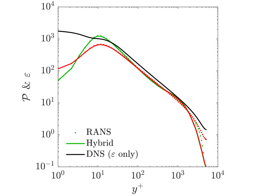 Figure 1
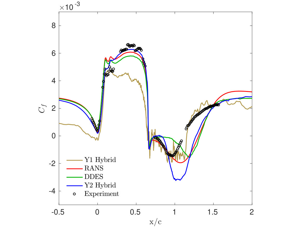 Figure 2
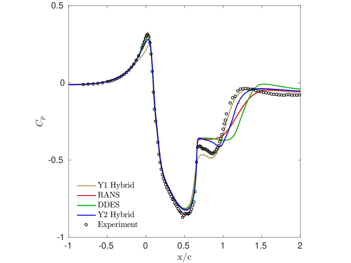 Figure 3
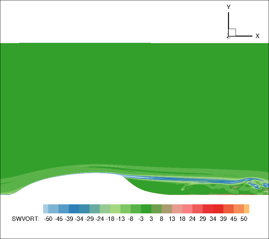 Figure 4
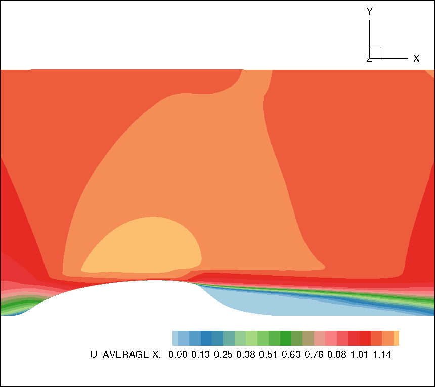 Figure 5
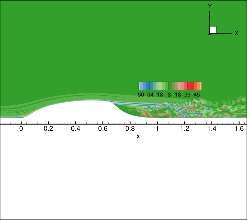 Figure 6
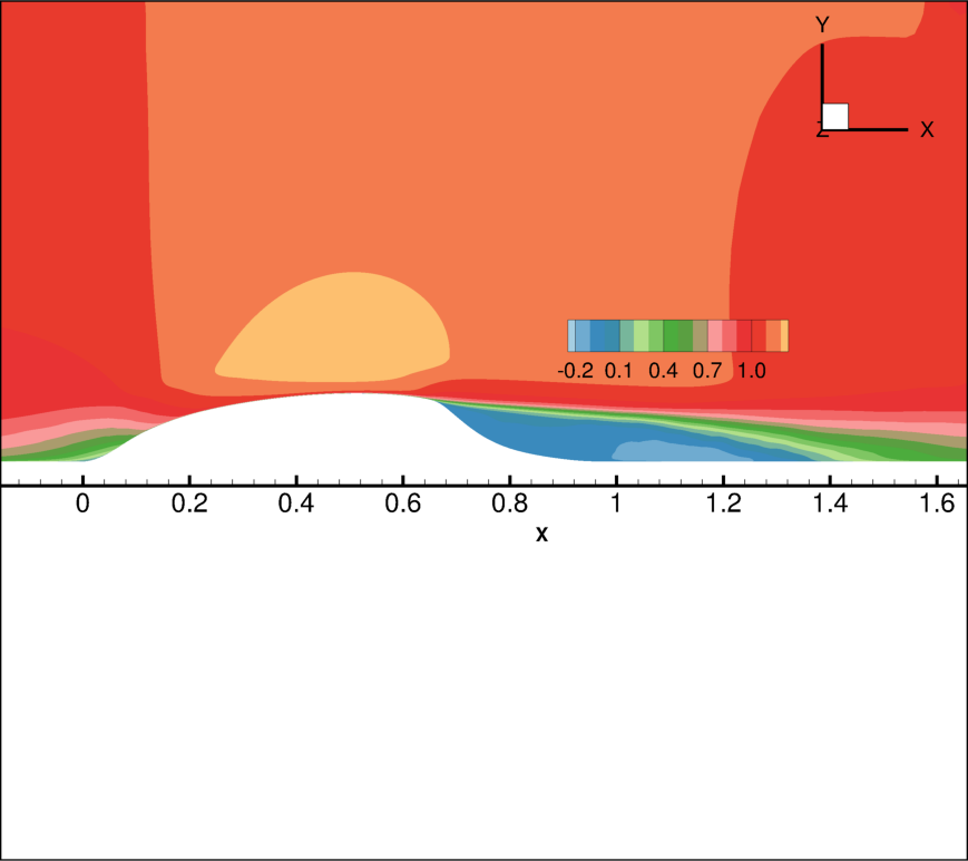 Figure 7
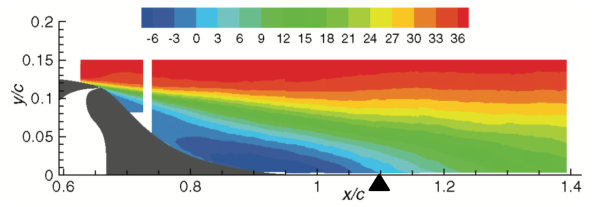 Figure 8
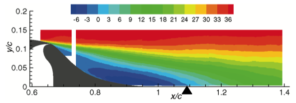 Figure 9
 Figure 10
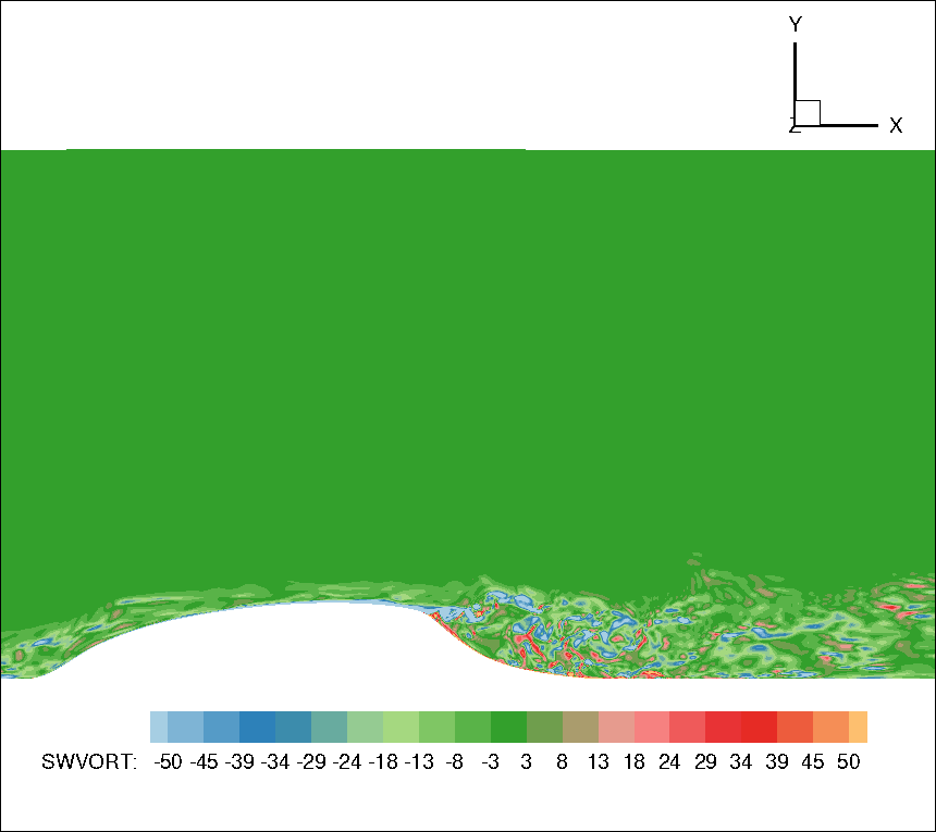 Figure 11
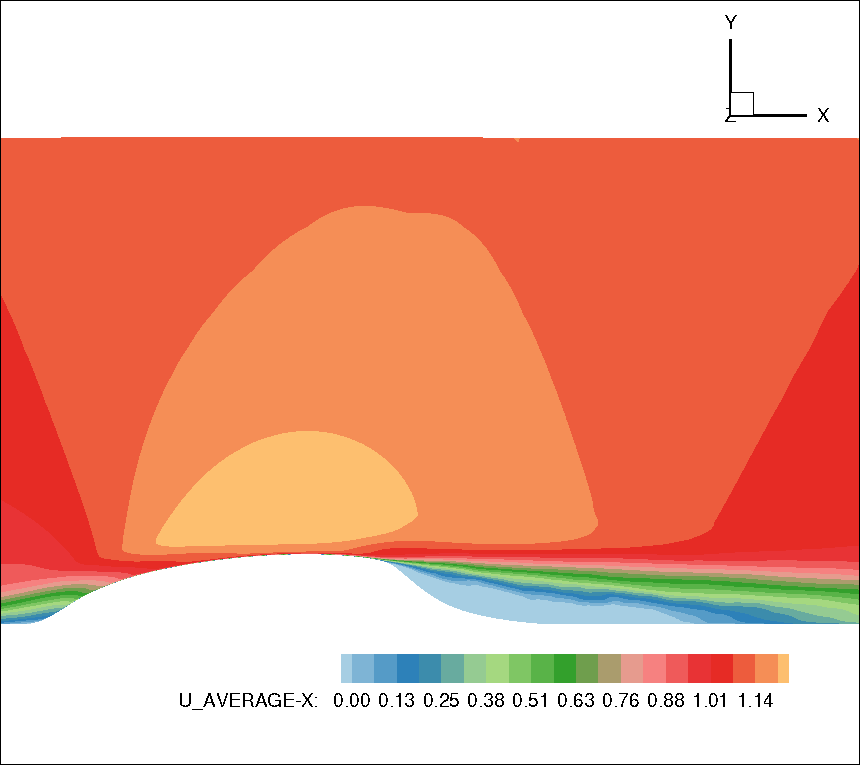 Figure 12
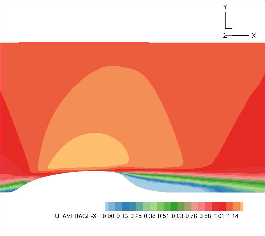 Figure 13
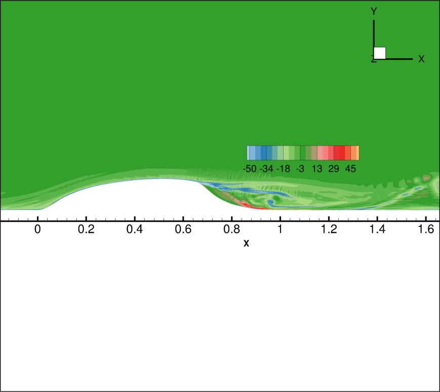 Figure 14
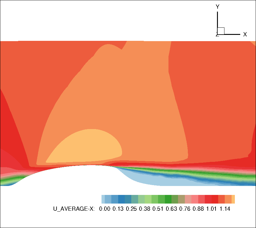 Figure 15
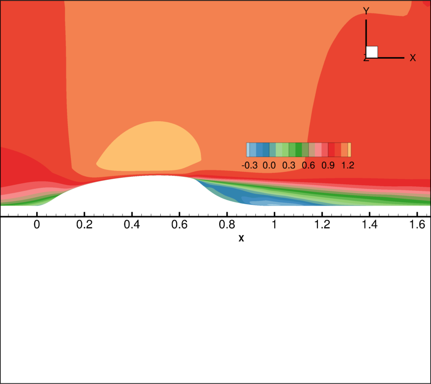 Figure 16
 Figure 17
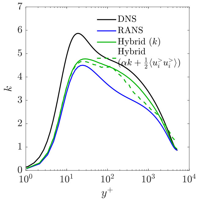 Figure 18
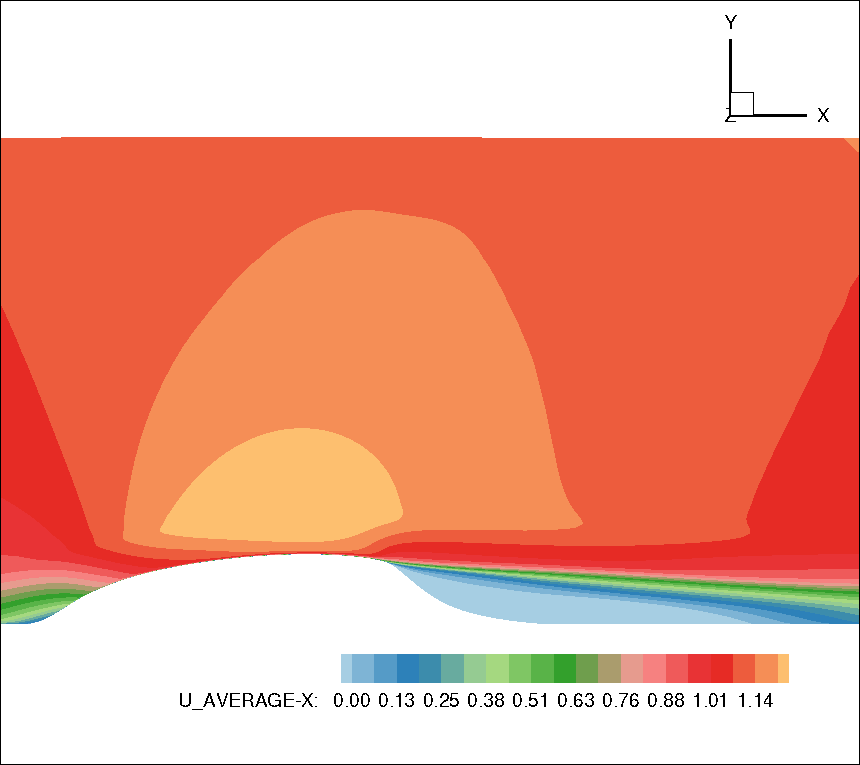 Figure 19
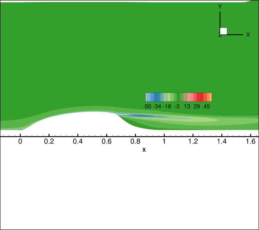 Figure 20
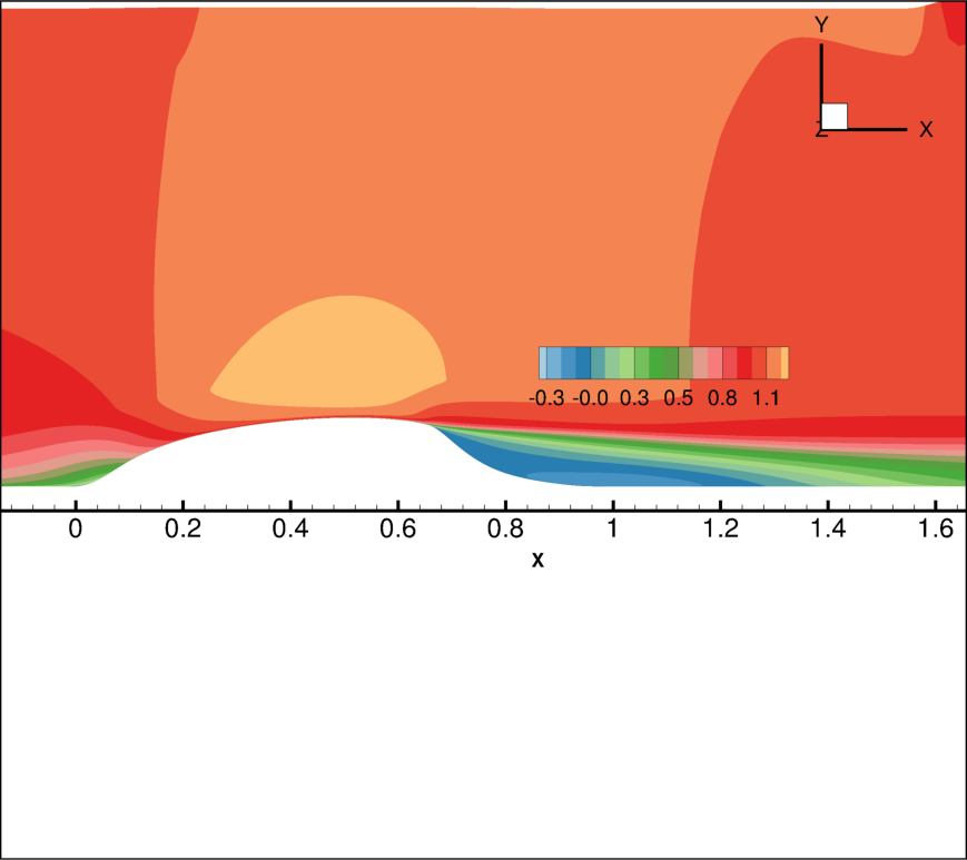 Figure 21
 Figure 22
 Figure 23
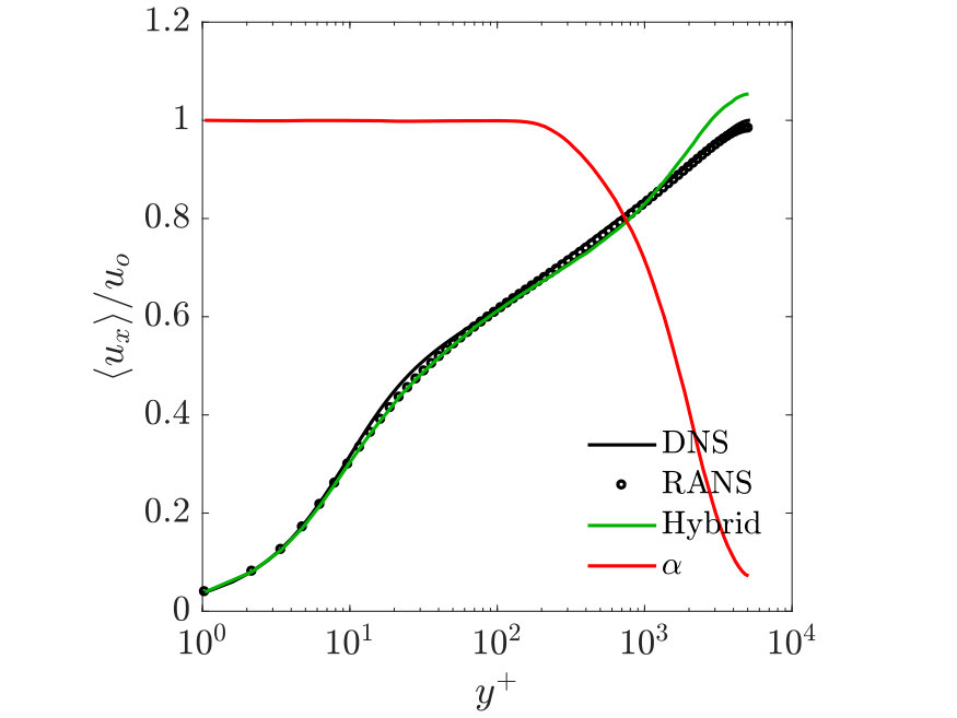 Figure 24
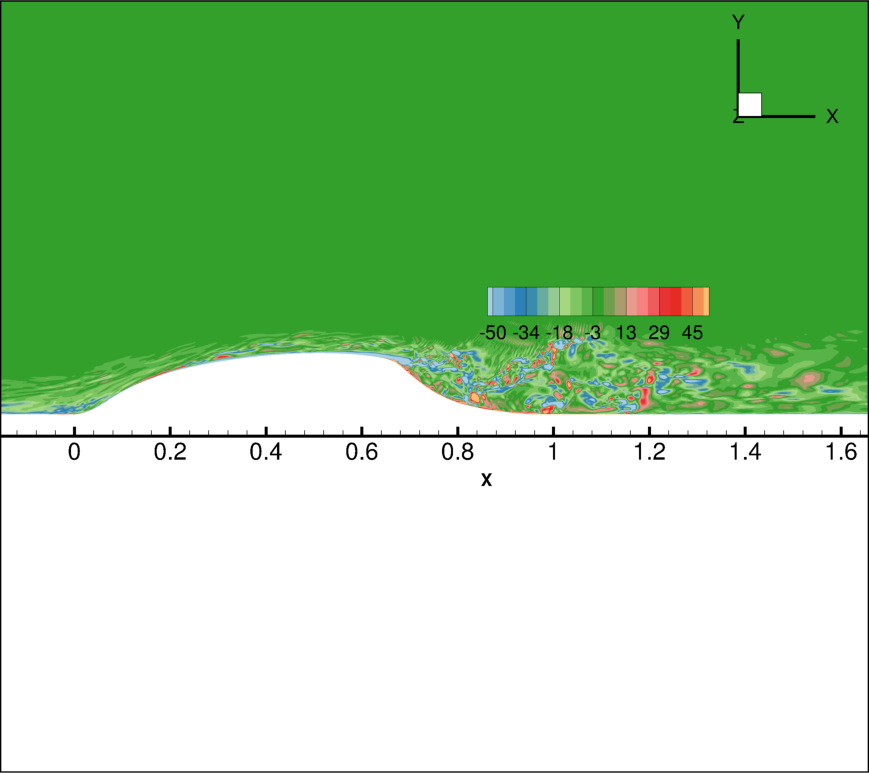 Figure 25
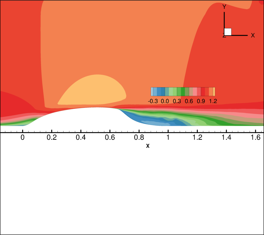 Figure 26
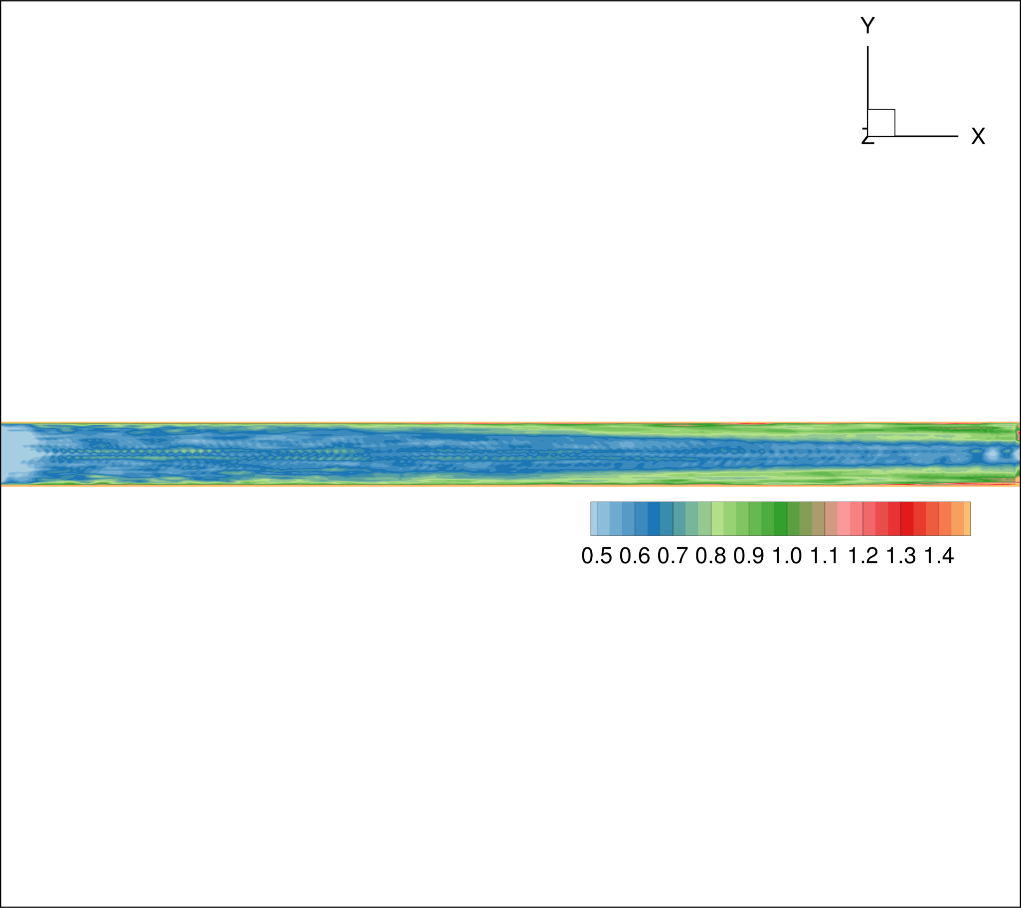 Figure 27
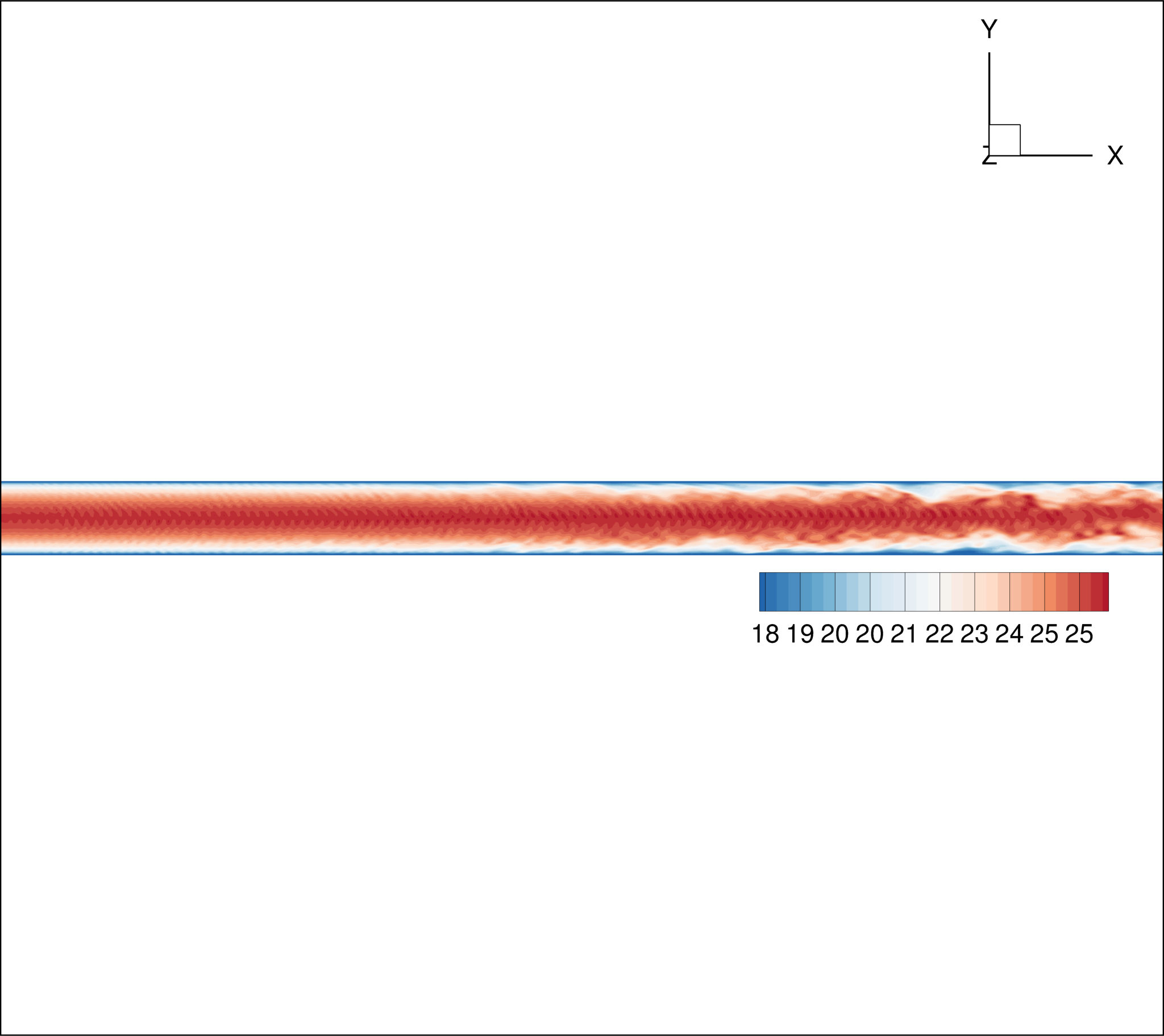 Figure 28
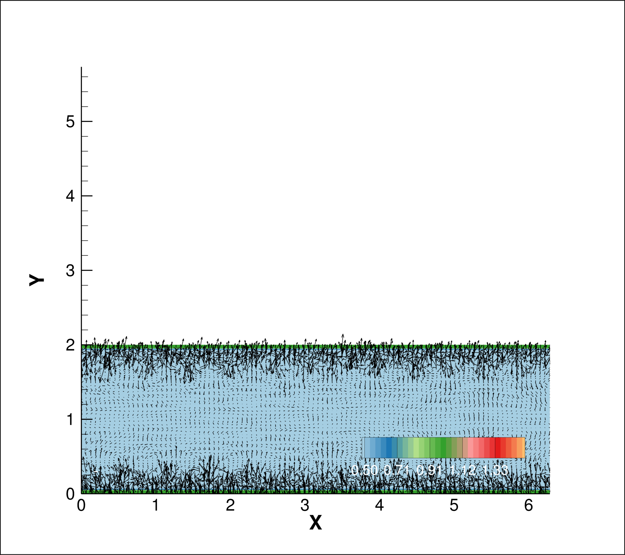 Figure 29
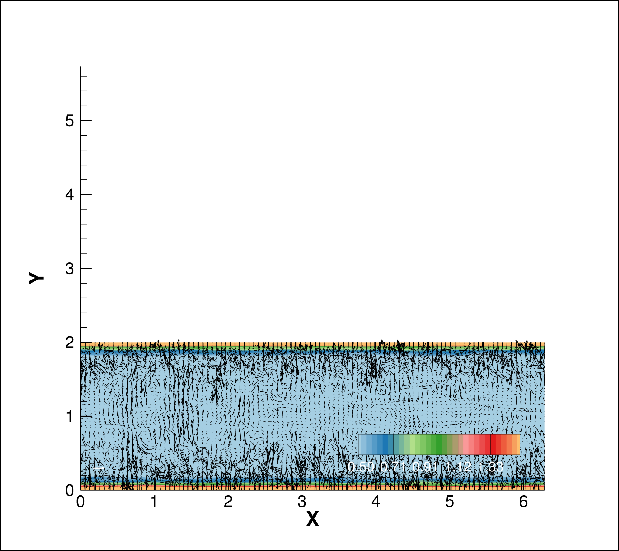 Figure 30
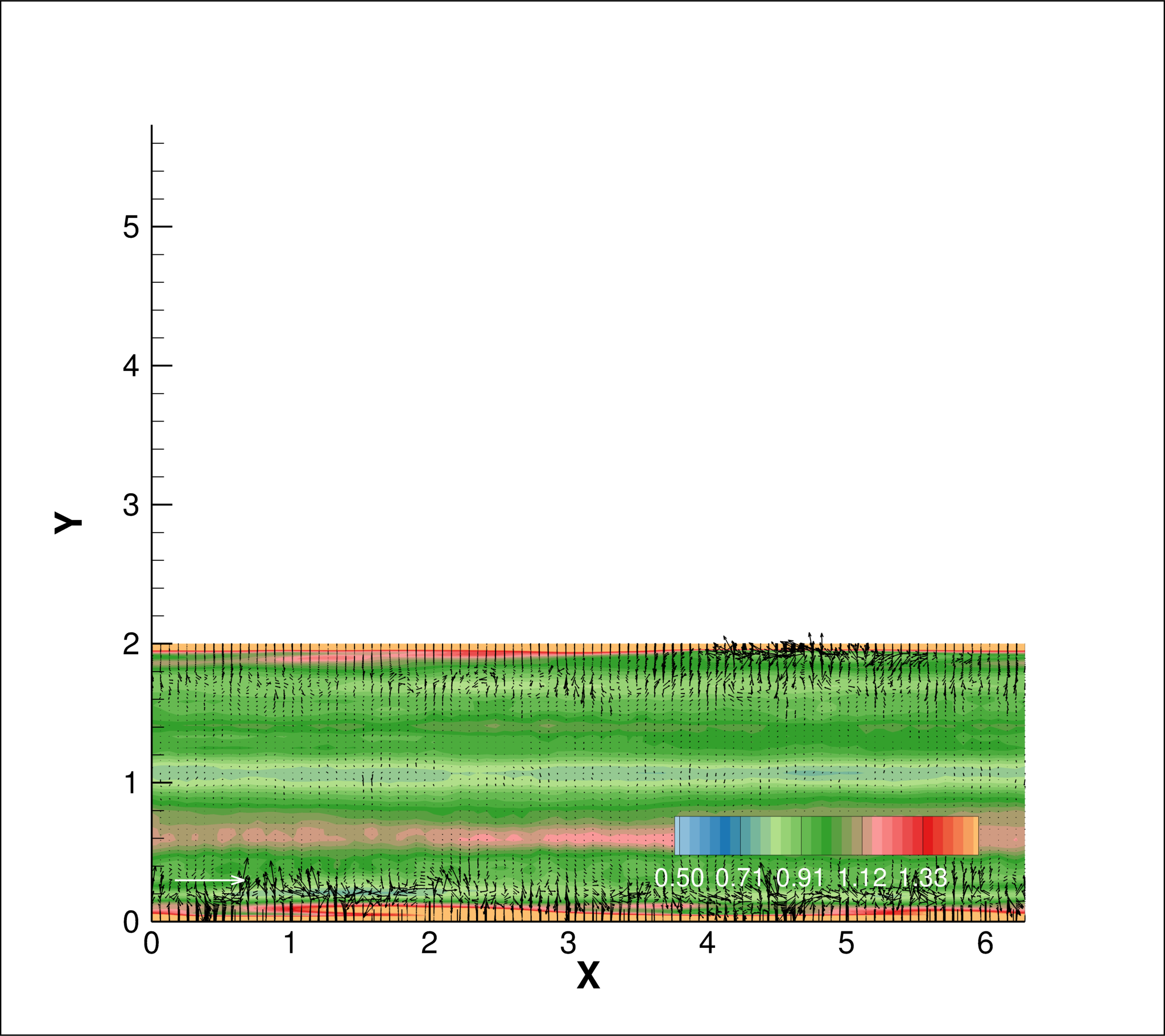 Figure 31
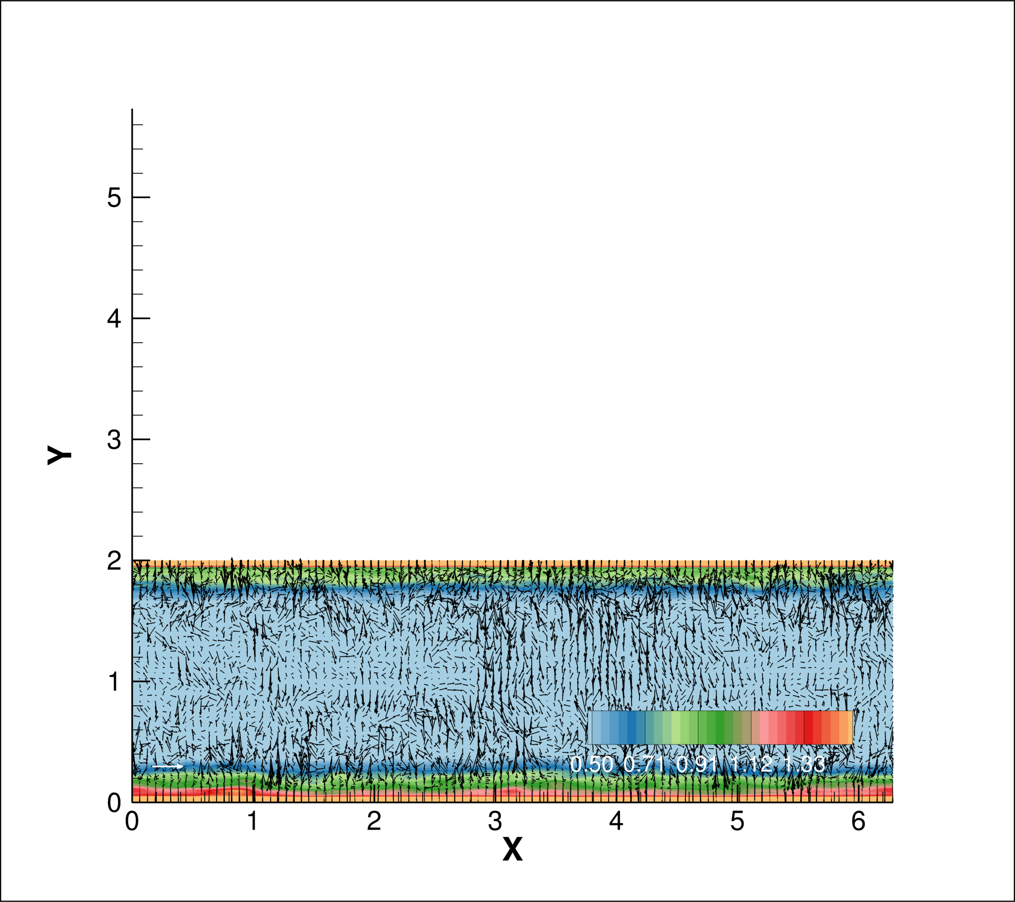 Figure 32
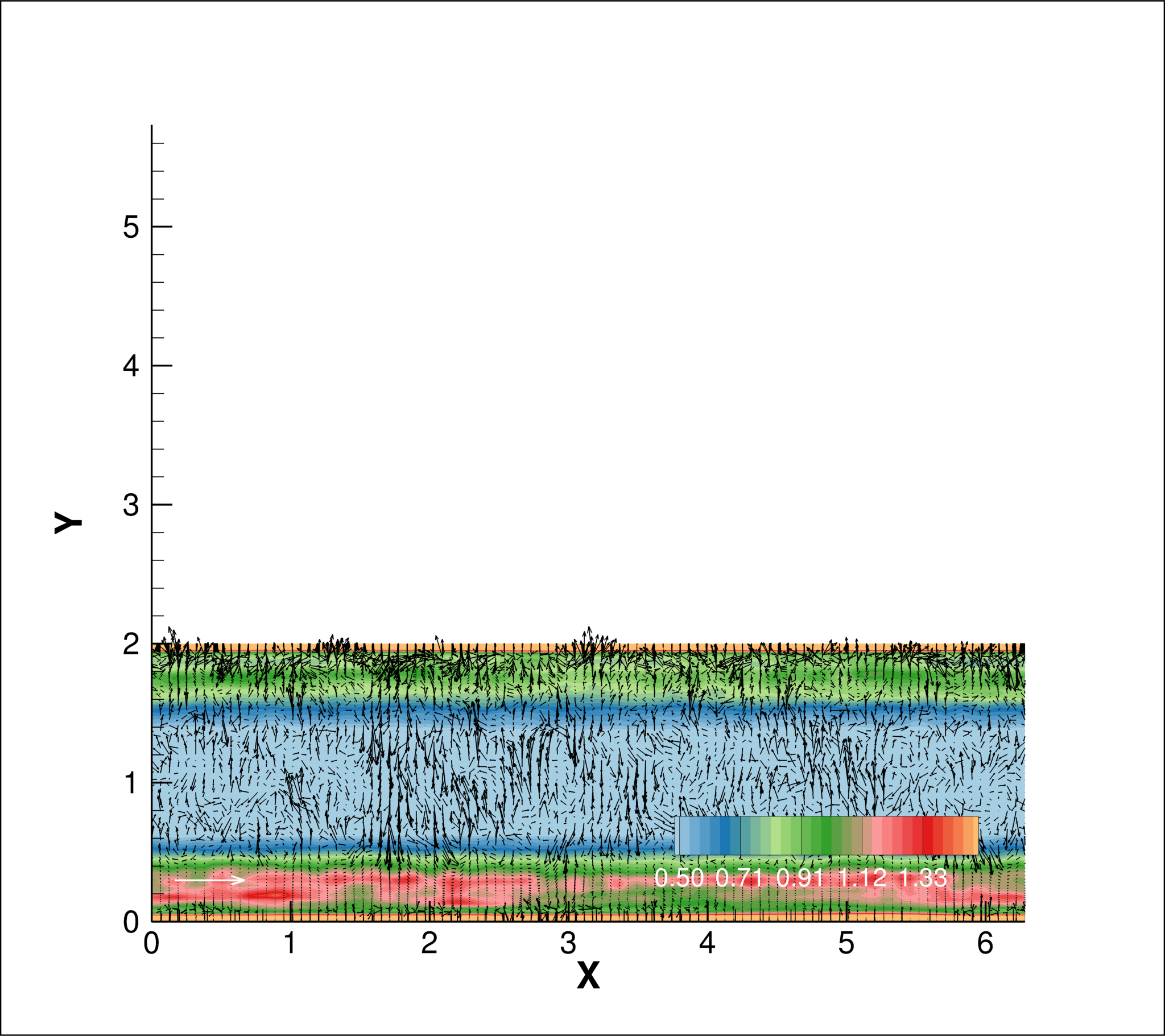 Figure 33
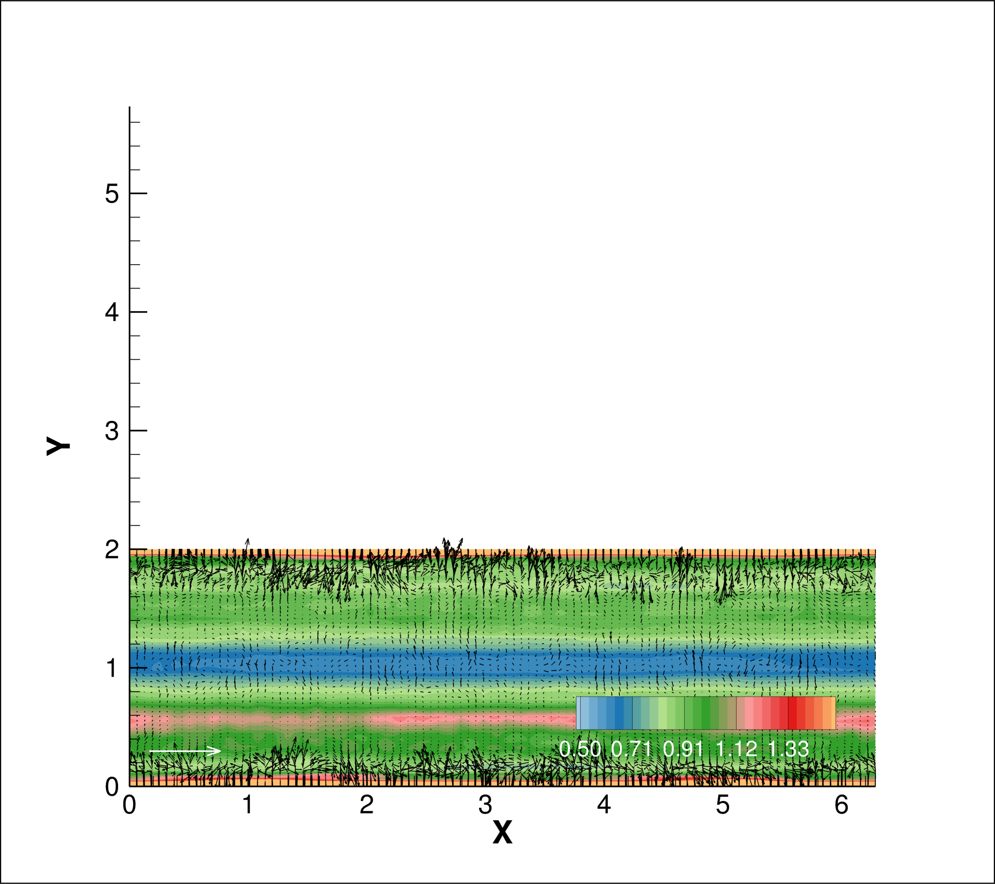 Figure 34
 Figure 35
 Figure 36
 Figure 37
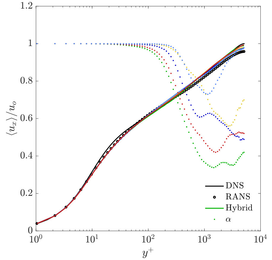 Figure 38
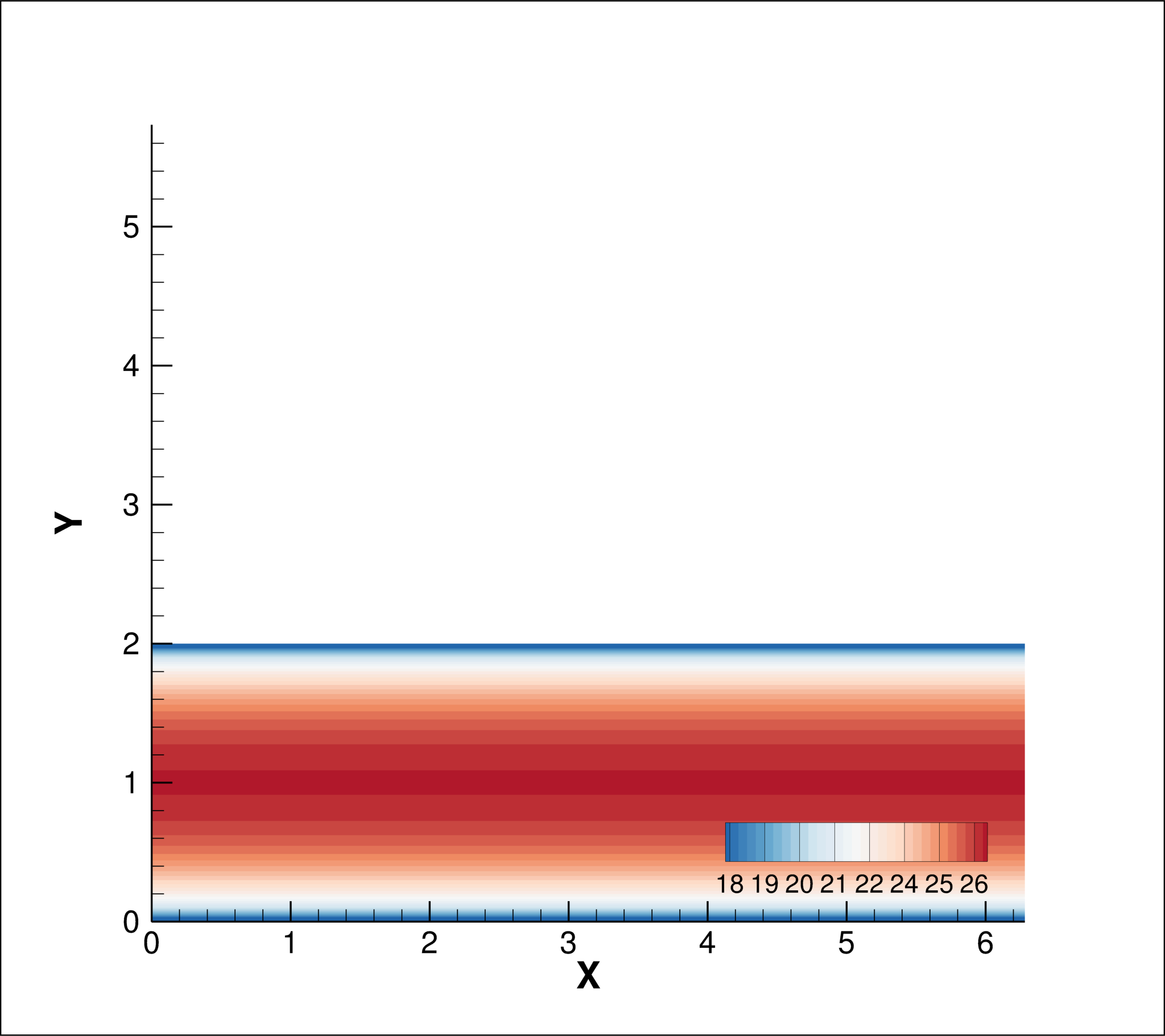 Figure 39
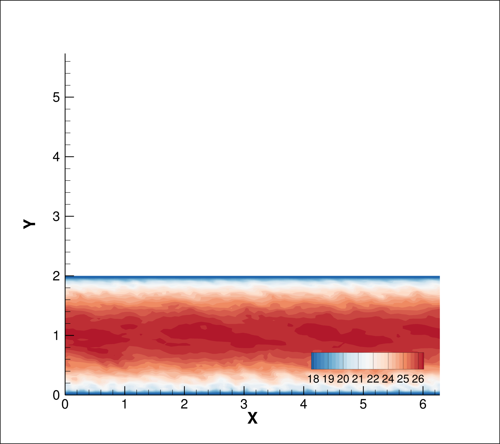 Figure 40
Peer Reviews
No public reviews on file for this paper yet. If you reviewed it on a platform where reviews are public (OpenReview, ICLR, NeurIPS, ICML), you can paste yours below so the community can read it here.
Videos
No videos yet. Explain this paper in a talk, walkthrough, or lecture? Add one.
A hybrid turbulence modeling paradigm for complex flows
Sigfried Haering*†‡, Todd Oliver‡, and Robert D. Moser†‡*
Department of Mechanical Engineering, The University of Texas at Austin
The Institute for Computational Engineering and Science, The University of Texas at Austin
- ABSTRACT
A hybrid RANS/LES modeling approach is developed for complex flows and their associated grids. The new approach has three main components: RANS to LES transition governed locally by identifying the least resolved orientation in the flow, hybridization rates are restricted by the turbulent timescales, and both grid anisotropy and heterogeneity are directly accounted for in LES modes of operation. Testing is performed with a wall mounted 2D-hump in channel flow to demonstrate functionality for the challenging simulation conditions of smooth-wall separation and reattachment.
Introduction
Hybrid models are a response to the limitations of available computational power for decades to come. While complete resolution of all turbulent scales (DNS) will not be achievable for practical engineering flows until the turn of the next century [spal:2000], the inadequacies and limitations of modeling all turbulence with direct simulation of only the slowly evolving mean flow (RANS) are well known [celic:2006, spal:2009, lesch:2002]. Although potentially capable of simulating transient flow features, unsteady RANS (URANS) still suffers from the shortcomings of RANS and is based on the assumption of non-turbulent unsteady time scales being greater than the largest turbulent time scales, which is seldom the case [shur:2005]. Being a compromise between complete simulation and complete modeling of turbulence, Large eddy simulation (LES) is often efficient and accurate for high Reynolds number flow where there exists a separation of scales between large energy containing eddies and small universal eddies. In the presence of strong flow anisotropy and in areas of low Reynolds number, such as near a wall, the benefits of an LES are lost as requirements for resolution of the energy containing eddies are nearly identical to a DNS . Hybrid methods are a recognition of the limitations of currently available techniques and resources. In such techniques, simulations contain varying levels of resolved turbulence from the range of total modeling to total resolving. How existing methods achieve this varies greatly.
In general, hybrid methods function by detecting if the local grid is capable of resolving some amount of turbulence. Where found to be true, the modeled stress is reduced allowing the formation of resolved turbulence and operation as an LES. The various methods of hybrid modeling differ in how they attempt to ascertain the adequacy of the local resolution to support simulation of turbulence and how the modeled stress is reduced in response. A growing list of hybrid models have been proposed and modified with varying degrees of success and overlap [froh:2008]. Indicators used to induce hybridization include comparisons of resolved and modeled turbulent kinetic energy[perot:2007], SGS and RANS eddy viscosities [batt:2000, batt:2004], and length scales. The latter is by far the most common and involves comparing a measure of the grid to the internal model length scale [baur:2003, riou:2008, grits:2012, jee:2012], Kolmogorov length scale[spez:1996, spez:1998], or wall distance [spal:1997, piom:2002, cabo:1999]. The reduced hybrid model stress used in the conservation of momentum is then either a weighted combination of the full model stress and the subgrid stress or results from a hybridized version of the full model equation. That is, the resolution indicator is used to blend the results of distinct RANS and SGS model equations or the indicator is used to internally blend the model equation so that it may function as both. Blending between distinct RANS and SGS models requires additional averaging of the resolved field such that the RANS equations consider only the mean flow in the presence of some degree of resolved turbulence. Alternatively, RANS and LES operation may be segregated by zones such that a region of LES operation is embedded in a RANS[quem:2002, deck:2005]. The spatial interface is either fixed beforehand or dynamically adjusted throughout the simulation. In these cases, it is this interface which is either blended or coupled in some manner.
Hybrid turbulence models often suffer from reliance on simple scalar measures of the available resolution to determine RANS to LES transition. Fundamentally, these measures are insufficient as they assume the instantaneous existence of resolved turbulent fluctuations at the resolution scale. Modeled stress depletion (MSD) results as there is not enough resolved turbulent stress to counteract the reduced modeled stress corrupting the entire simulation . Multiple measures have been used in the literature and are interchanged as dictated by whatever happens to give the best results for the particular study . Corrections are often proposed when this fails. For instance, “delaying” functions have been used to some success to prevent premature flow separation along smooth walls due to local grid refinements . However, the form of the correction is ad-hoc and requires additional coefficient tuning rendering them non-predictive in general. In addition to being insufficient to accurately govern model hybridization, scalar grid measures result in either under utilization of the available resolution or attempting to resolve more turbulence than can be supported. While the former may result in acceptable additional computational cost, the latter may corrupt the simulation. Further, as resolved turbulence is convected through regions of coarsening or refining resolution, the hybridization should adjust the balance of resolved and modeled turbulent kinetic energy accordingly lest the issues of over/under resolution manifest again. These problems are pervasive in LES in general and both fields would greatly benefit from a more thorough treatment of grid anisotropy and heterogeneity.
In this work, we propose a basic universal paradigm to access resolution adequacy and to govern the response of turbulence model equations. In short, an anisotropic estimate of the unresolved turbulent fluctuations is constructed from the resolved field and an anisotropic “filter” bound below by the underlying grid. From this, the local least resolved orientation is identified and used to access the potential for resolving turbulent content. The response of the model equations is restricted by the local turbulence timescales thereby allowing resolved turbulent fluctuations to form naturally at the rate the model stress is reduced. Additionally, the anisotropic estimate of the unresolved turbulence dictates the model stress anisotropy in LES regions. Finally, the total model stress is adjusted in response to convection through resolution inhomogeneities with energy transferred between resolved and modeled equations. We anticipate the new modeling and hybridization approach presented here will solve commonly observed problems in hybrid simulations of complex geometry problems requiring inhomogeneous and anisotropic meshes containing complex features like dynamic smooth wall separation. In doing so, the approach addresses critical barriers to the predictivity of CFD for important engineering systems like those identified in the Grand Challenge problems outlined in the CFD Vision 2030 Study [nasa:2014].
Hybrid Method
11todo: 1some intro bit here
Resolution Adequacy
Begin by considering some field of turbulence, , in a domain, , which is segregated without any loss of information into large and small scales of motion relative to a general anisotropic length scale tensor, say , so that . This length scale tensor may be defined as the square root of the metric tensor defining the transformation of a unit cube to the desired arbitrary size and orientation defined by the global coordinate system. Clearly, the smallest fluctuations in are equivalent to the largest fluctuations of at every point in in every orientation. All higher order statistics may be segregated in a similar manner, in particular, considering turbulent kinetic energy yields 22todo: 2need some help expressing this max/min statements…
[TABLE]
Further, the largest of the smallest fluctuations of is at least the smallest of the largest fluctuations of . In a simulation where defines the resolved turbulence field and defines the unresolved modeled turbulence, this trivial observation forms the basic requirement for evaluating if the provided resolution, as defined through , is capable of supporting additional turbulent content. That is, we desire everywhere
[TABLE]
or that the resolution is at least capable of supporting the smallest unresolved fluctuations at . It is therefore conservative by construction. We now discuss how to estimate the quantities in (2) provided information in turbulence simulations.
If isotropic turbulence is assumed at the scales of , the numerator of (2) may be expressed using (1) as: . Thus, we seek to form an estimate of the unresolved turbulent kinetic energy with information provided by the resolved field. It is well known the total two-point second-order structure function at separation distances
[TABLE]
relates directly to the total turbulent kinetic energy through integration of the energy spectrum, , as
[TABLE]
where a Kolmogorov inertial range has been assumed (). Provided a structure function filtered at , so that
[TABLE]
where . For an arbitrary orientation in the field, say , the separation distance may be defined through the length scale tensor as . Therefore, to a first-order approximation, velocity differences across separation in any arbitrary direction are simply and an anisotropic representation of the filtered structure function is
[TABLE]
so that .33todo: 3comment on dropping the averaging Combining (6) and (5) forms an anisotropic estimate of the unresolved turbulent kinetic energy resulting from the anisotropy of the resolved field and resolution tensor. With this estimate, the numerator of (2) is simply where is the maximum eigenvalue of . Note that where is greater than the large scale turbulence length scales, (5) will over estimate due to the assumption of a simple inertial range extending through all scales of motion. While this may seem troublesome, it becomes useful for hybridization purposes as we will discuss later.
The numerator of (2) requires knowledge of the anisotropy of the unresolved turbulence. When using standard scalar RANS eddy viscosity models as SGS models, as is common with hybrid modeling, such information is not available. Two equations models will provide an isotropic measure of the modeled turbulent kinetic energy, , so that the numerator of (2) would have to take the form of where may require tuning for particular flow conditions and resolution combinations. When using single equation models, such as the popular SA model, a lengthscale must be derived from the gradients in the resolved field to construct an isotropic estimate of using the model eddy viscosity (k_{m}\approx{}C\big{(}\nu_{t}\tfrac{|\nabla^{2}u|}{|\nabla{}u|}\big{)}^{2} for instance). In practical applications, anisotropy information is critical for (2) being a universal measure of resolution adequacy and driving hybridization. This is most apparent near boundaries where the smallest of the largest of the unresolved fluctuations is significantly reduced by blockage effects. Fortunately, the model of Durbin and Lien provides precisely the required information. Through wall boundary conditions and the balance of production and destruction of turbulent kinetic energy in the elliptic relaxation equation for , is a direct approximation of the smallest large scale fluctuations of the modeled turbulence, i.e. \mkern 1.5mu\overline{\mkern-1.5muv^{2}\mkern-1.5mu}\mkern 1.5mu\approx{}\min\big{(}\max\big{(}(u_{i}u_{j})^{<\mathbf{M}}\big{)}\big{)}.
Thus, through the resolved field, a resolution tensor everywhere at least the local grid size, and the use of the popular RANS model, a measure for the ability of a simulation to locally support more turbulent content has been constructed without any tuning coefficients are special considerations for boundaries beyond what is already present in the model. We will now discuss implementation.
Hybridization
Modifications to the governing and model equations to function in both RANS and LES regions, referred to as “hybridization”, is performed using the basic approach of Perot and Gadebusch [perot:2007]. The model viscosity appearing in conservation of momentum and the corresponding production term in the equation are multiplied by what they refer to as “backscatter coefficient”, , as
[TABLE]
[TABLE]
with the turbulent dissipation, , evolution equation modified only in a constant term. The backscatter coefficient is determined by some measure of the adequacy of grid resolution for the local instantaneous flow. If the grid is capable of resolving additional unsteadiness or turbulence, energy from the turbulence model is returned to the resolved scales via some less than unity. The lower bound on should be selected with not only realizability constraints ( bounded above zero) but also so that energy returned to the resolved scales can be redistributed to a physically realistic state from the somewhat unrealistic state resulting from a reduction in diffusion. Through the interchange of increased resolved content and reduced model kinetic energy, will tend to a quasi-steady value dependent, yet not directly determined by, the local grid size.
The difficulty of the Perot method lies in choosing a proper resolution indicator and how should scale with this variable. In the original work, an indicator constructed from the total resolved turbulent kinetic energy, its gradients, and grid size in form not amenable to complex unsteady flows and unstructured grids. Thus, we will only adopt the basic blending approach in (7) and (8) and construct with (2) determined as previously discussed,
[TABLE]
with .
The blending parameter, , is to be driven by but not defined by it. The objective of blending is to achieve . When this is achieved, the resolved and modeled turbulence are balanced with respect to the least resolved orientation in the field and the current level of RANS/LES blending should remain constant. Alternatively, when , the amount of blending must change to guide the resolved field to equilibrium with the model111The exception to this is in the full RANS limit where though there is no resolved turbulence to return to the model and so must be maintained at unity.. In the interest of preventing MSD corruption and only resolving physically meaningful turbulence, the rate at which energy is returned to or removed from the resolved scales must be limited such that the total turbulent stress remains relatively constant and is only modified by improved information provided additional resolved turbulence. This limiting is achieved by controlling the rate of change of using the local turbulent timescale of the modeled turbulence, . Specifically,
[TABLE]
When the resolved turbulence at the resolution limit is in equilibrium with the modeled turbulence, the smallest resolved turbulent timescale is approximately equal to the largest-scale modeled timescale such that is an appropriate timescale for the entire dynamic process. Note that, to ensure full RANS behavior in regions where , is limited to be less than or equal to 1. Further, should be limited so the modeled turbulence remains positive semi-definite. Ignoring transport terms, ensures the total change in over the turbulent timescale, , is approximately . Provided the simulation timestep is less than , restricting is sufficient.
Model anisotropy
Since we propose to use standard scalar eddy viscosity models rather than full Reynolds stress modeling, the hybridization process has been reduced to a scalar parameter resulting in a scalar eddy viscosity based on the standard RANS form. However, given our knowledge of the anisotropy in the estimation of the unresolved turbulent fluctuations through and the gradients in the resolution itself through , we may introduce directional dependence in the hybrid model eddy viscosity.
Unresolved k-based anisotropy
We desire to introduce a tensor model viscosity, , to reflect the anisotropy in the estimation of the unresolved turbulent kinetic energy when the resolution is sufficient, i.e., when is in the inertial range. Alternatively, in full RANS mode, when , the hybrid eddy viscosity should, of course, be the usual eddy viscosity from the RANS model. To accomplish this, we introduce the hybrid eddy viscosity
[TABLE]
where the anisotropy tensor, , is given by
[TABLE]
[TABLE]
and is composed of the principal directions of the tensor . The choice of basing anisotropy on stems from being a realspace anisotropic analog of the spectral structure-function eddy viscosity of Metias and Lesieur based on \nu\sim\big{(}\tfrac{E(\kappa)}{\kappa}\big{)}^{1/2} . The accompanying turbulent stress model is
[TABLE]
which collapses to the standard Boussinesq assumption for isotropic .
Equation (11) acts to redistribute the scalar hybrid eddy viscosity to be consistent with the estimated anisotropy in the unresolved field. When , , and the anisotropy takes that of . Alternatively, with increasing , , such that approaches identity and asymptotically approaches the standard isotropic RANS eddy viscosity. This is, of course, not ideal and stems from a difficulty of distinguishing RANS regions from areas of of convection of turbulent content through coarsening grids while is still capable of LES locally. However, as previously mentioned, is erroneously large when is not within the inertial range. This error benefits transition to full RANS behavior in the proposed hybrid method. Next, we discuss consideration for heterogeneous resolution in regions of LES operation.
Heterogeneous resolution anisotropy
Large eddy simulations and hybrid methods can be corrupted by commutation errors in the presence of grid resolution inhomogeneities . Amplification type errors result from passing filtering of the gradient of a field onto the gradient of the filtered field . Though second-order, these errors interact with the more commonly known dispersion type errors associated with under-resolved convection leading to increased simulation corruption. In principle, this problem can be corrected by imposing a uniform resolved length scale in the resolution tensor defined in §LABEL:. When the grid spacing is everywhere smaller than this resolved length scale, enforcing uniform model resolution will prevent gradients in the grid from corrupting the resolved turbulence. However, in realistic applications, this approach is generally impractical, since resolution requirements for the turbulence to be simulated are often inhomogeneous. Instead, we propose a model which transfers energy between resolved and unresolved scales as turbulence flows through resolution inhomogeneities.
The proposed model is based on work by Ghosal [ghosal_b], who analyzed the problem from the perspective of convection through coarsening filter widths. Through a transformation of arbitrary to uniform filter widths followed by a truncated Taylor series expansion, 1D commutation error was found to behave as
[TABLE]
where is the grid spacing defining the filter width and is related to the specific filter (unity for a realspace tophat filter). As previously mentioned, we are only concerned with commutation errors associated with the convective term due to their amplification of dispersion errors. Applying (15) to the convective term yields a “viscosity” of the form . We propose an anisotropic extension based on this artificial commutation error viscosity and formed with the resolution tensor as
[TABLE]
Several additional consideration must be made before implementation of (16). First, (16) may only be used in LES regions as an adequately resolved RANS simulation is insensitive to gradients in the underlying grid. Further, when turbulence is being convected through regions of resolution refinement, (16) will be negative and serve to backscatter energy from the model. Therefore, when anti-dissipative, (16) must vanish in the limits of no modeled turbulence, i.e. local DNS resolution. To this end, (11) is modified as
[TABLE]
[TABLE]
where , and is composed of the principal directions of . Note the blending parameter is only used in the dissipative limit, this is to prevent flow through coarsening grids from counteracting hybridization.
While the effect of this term on the resolved scales is similar in some ways to the artificial viscosity added by upwinding the convection term in the momentum equation, i.e. spurious oscillations due to convection of resolved structures through a coarsening grid are removed222Along these lines, (16) may be viewed as setting a Reynolds number based on resolutions gradients to unity, i.e. ., the construction here is formulated such that energy is exchanged between the resolved and modeled scales rather than simply destroyed. This is achieved through the production term in the model turbulent kinetic energy equation (LABEL:energy) containing the viscosity defined in (16). Thus, the resolution inhomogeneity treatment proposed here is energy conserving in both dissipative and anti-dissipative operation.
44todo: 4some closing statment
Demonstration
A thorough validation of the proposed hybrid method is not performed here. Rigorous examination of each of the presented components is warranted and is part of an ongoing effort. However, as is custom with hybrid methods, a single, albeit challenging, problem is used to demonstrate the capabilities of the new method. We consider the problem of channel flow over a 2D wall-mounted hump featuring flow with smooth-wall reattachment and separation. Data from the experiments of Greenblatt et.al. is used to specify inlet conditions and for validation . Delayed detached eddy simulation (DDES) built on the RANS model with an identical mesh is used as an exemplar for existing hybrid methods.
Channel flow with a wall-mounted 2D hump
The current hybrid method is as presented in our original proposal. The central idea is to use the resolved field and resolution to form an estimate of the unresolved turbulent kinetic energy which is then used to guide the model and resolved field to equilibrium about this estimate at a rate dictated by the resolved turbulence. The estimate of the unresolved turbulence is based on the anisotropic structure function approximation used in §LABEL:sec:aniso_filter. Additionally, convection of turbulence through inhomogeneous resolution regions is directly incorporated.
Year one case studies were chosen to be low Mach such that they can be studied using the current implementation in CDP, allowing development of the compressible model and validation of the existing model to proceed in parallel until the compressible model has been formulated and implemented. The first case considered is the 2D-hump in cross-flow of Greenblatt et.al. [green:2006]. Their data show smooth-wall reattachment, which current hybrid methods often fail to predict correctly, making this an excellent case for hybrid model validation.
The model domain is a truncated version of the experimental windtunnel with inlet region prior to measured mean velocity profiles at being discarded (Fig. 4). RANS simulations of flow over a flat plat at the identical are performed using the [lien:2001] model to generate appropriate model inlet boundary conditions where matching the experimental mean velocity profile (Fig. 2). The top of the domain is prescribed a slip boundary condition.
For our first simulation attempts, a span of was considered with initial wall normal spacing of (), wall tangent spacing at the hump of , and spanwise spacing of resulting in highly anisotropic cells in the separation region (Fig. 4b). The total cell count for this mesh is .
Results
Simulation spanwise vorticity and time averaged velocity contour plots for basic RANS, DDES [spal:2006] developed for the model [jee:2012], and the hybrid method are shown in Fig. 3. We see that, for the same mesh, the hybrid method (Fig. 3e) resolves significantly more turbulent content than DDES (Fig. 3c) which is very similar to the baseline RANS case (Fig. 3a). Further, the reattachment location moves upstream towards the experimentally observed location but is still in disagreement (Fig. 3g).
To correct this, the mesh is refined by a factor of four in and just upstream of the separation region (Fig. 4c). Additionally, a thin band of approximately is restricted to a maximum of in the wall normal direction. This is in contrast to the previous mesh which was grown by in each wall normal step. With this refined cross-sectional mesh, three spans are considered, , and . The total cell count for these domains are , , and respectively. Time average fields are shown in Fig. 4. Most notably, the reattachment point is seen to be strongly dependent on the spanwise domain of the simulation with thinner domains delaying reattachment. Near agreement with experiments is seen for the widest span case (Fig. 4c and Fig. 4d).
The difference between Fig. 3f and Fig. 4b also reveals the sensitivity of reattachment to resolution of the separation. Though originally thought to only be a useful test case for smooth-wall reattachment as the separation point was thought to be predetermined by the hump “edge”, these differences and detailed examination of the separation region (Fig. 5) indicate smooth-wall separation is also a factor. Significant backflow along the hump surface is observed as seen by the purple and red regions in Fig. 5b. In response to the increased resolution, the separation point shifts upstream which, along with increased resolution of turbulence in the separated shear layer, allows the reattachment point to also move forward.
While DDES has not been run yet on the fine mesh, the increased resolution is not expected to improve the results. Specifically, DDES is expected to generate the same RANS-like solution as on the coarse mesh due to its dependance on a scalar measure of the highly-stretched cells and an aggressive delaying function.
Experimental and wide-span hybrid simulation pressure coefficients and skin friction are compared in Fig. 6. Good agreement is obtained in (Fig. 6a) with consistent under prediction of maxima and minima and a slight smearing of the pressure recovery in the hump separation region. Skin friction, however, exhibits more qualitative agreement only (Fig. 6b). While the initial increase at the forward portion of the hump and the aft recovery region agree well, the separation region is significantly different. This disagreement may be due to imprecise experimental oil measurement techniques and/or the fact that the simulation is from an instantaneous field averaged over the span as opposed to being time-averaged.
Discussion
Summary
For the most part, existing so-called “anisotropic” treatments [les:1996, scott:1993] do not have filter anisotropy directly built into the structure of the SGS model as we have done here. Instead, adjustments to the scalar measure of the modeled turbulent velocity scale are made to consider filter anisotropy while the final model still adopts anisotropy from the filtered strain. As we have seen here, neglect in filter anisotropy results in an erroneous distribution of resolved turbulent kinetic energy and total model dissipation.
The Clark model [clark:1979] takes anisotropy directly from the approximation of the modeled velocity scale using a contraction in the gradient indices (instead of velocity indices as in ) as . Clearly, (6) could be rearranged similarly so that filter anisotropy would be directly incorporated into the Clark model. The rationale for doing so is to construct a direct model for the Reynolds stress tensor. However, consistent with the original findings in [clark:1979], doing so results in a model where the constant must be artifically set to zero when the model becomes anti-diffusive to preserve stability. The likely reason for this necessity is that there is no simple scaling relation between the filtered anisotropic velocity gradients and the unresolved anisotropic Reynolds stress (such as in the isotropic homogeneous structure function (LABEL:Fii)). Such arbitrary “clipping” of model coefficients is highly undesirable when trying to construct robust and physical models. However, returning to this formulation, perhaps in conjunction with the the form represented by (6) to construct the combination of filter anisotropy and Reynolds stress anisotropy, is an intriguing possibility for future research.