The Gerdjikov-Ivanov type derivative nonlinear Schr\"odinger equation: Long-time dynamics of nonzero boundary conditions
Boling Guo, Nan Liu

TL;DR
This paper analyzes the long-time behavior of solutions to the Gerdjikov-Ivanov derivative nonlinear Schrödinger equation with nonzero boundary conditions, revealing different asymptotic regions including plane waves and modulated elliptic waves.
Contribution
It provides a detailed asymptotic analysis of the Gerdjikov-Ivanov equation with nonzero boundary conditions using Riemann-Hilbert problem techniques.
Findings
Solutions exhibit plane wave behavior outside the central region.
Inside the central region, solutions form modulated elliptic waves.
Different asymptotic regimes are characterized by the $xt$-plane regions.
Abstract
We consider the Gerdjikov--Ivanov type derivative nonlinear Schr\"odinger equation \berr \ii q_{t}+q_{xx}-\ii q^2\bar{q}_{x}+\frac{1}{2}(|q|^4-q_0^4)q=0 \eerr on the line. The initial value is given and satisfies the symmetric, nonzero boundary conditions at infinity, that is, as , and . The goal of this paper is to study the asymptotic behavior of the solution of this initial-value problem as . The main tool is the asymptotic analysis of an associated matrix Riemann--Hilbert problem by using the steepest descent method and the so-called -function mechanism. We show that the solution of this initial value problem has a different asymptotic behavior in different regions of the -plane. In the regions and , the solution takes the form of a…
Click any figure to enlarge with its caption.
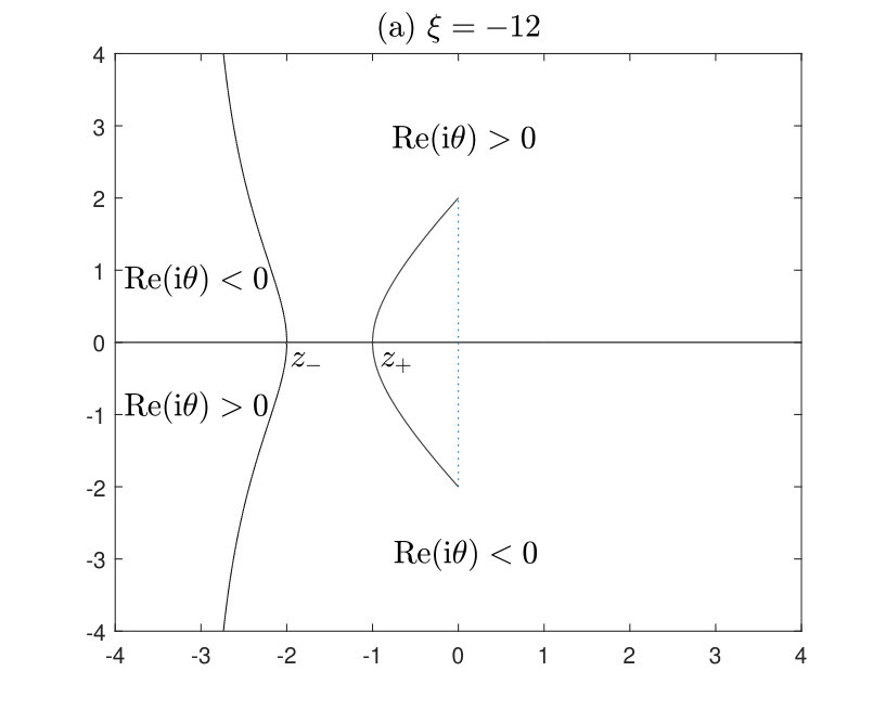 Figure 1
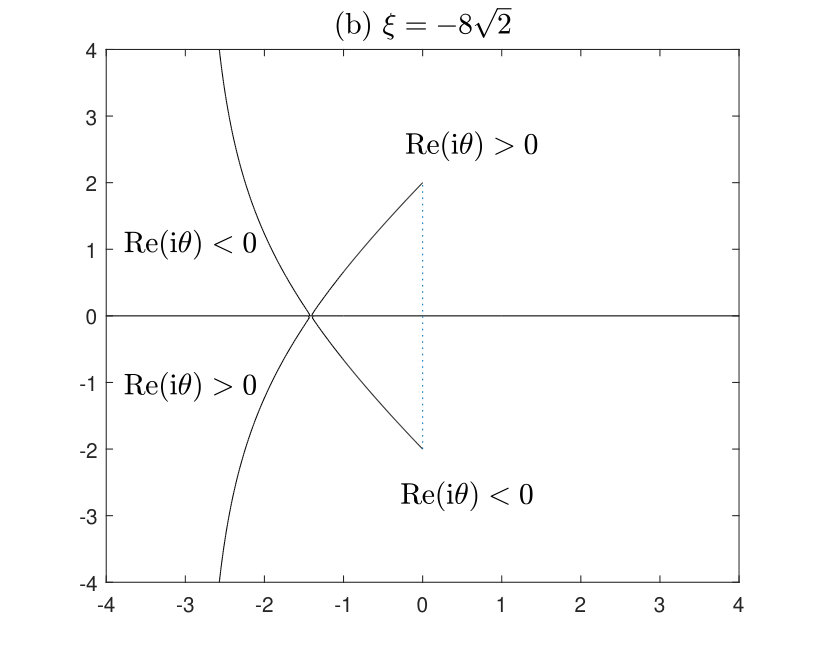 Figure 2
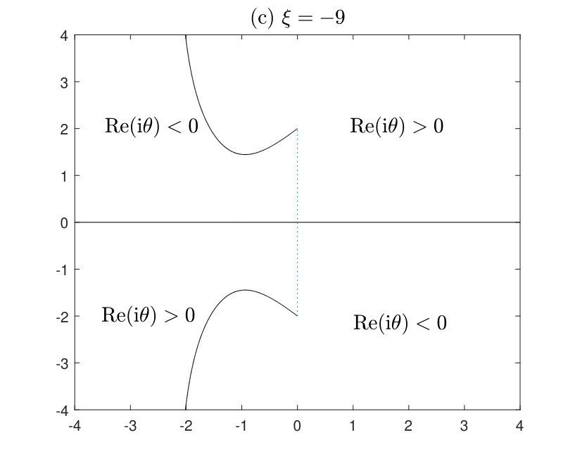 Figure 3
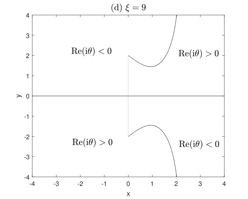 Figure 4
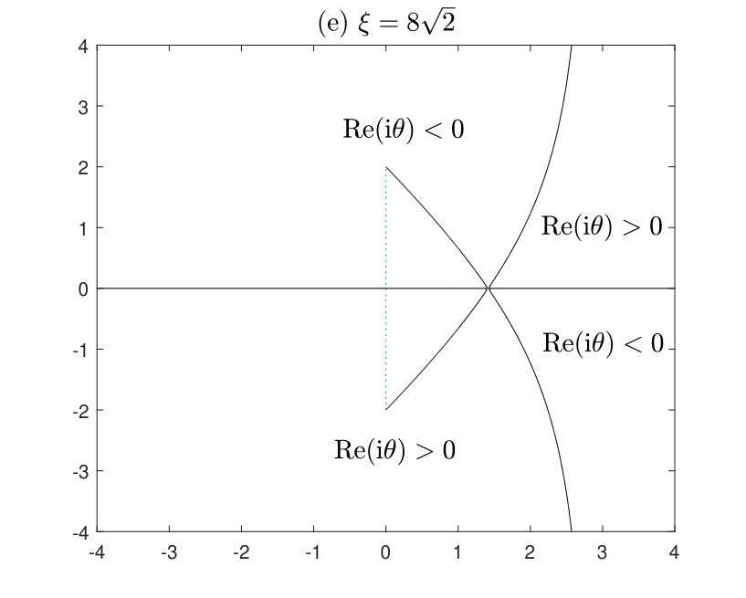 Figure 5
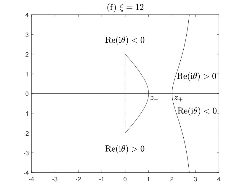 Figure 6
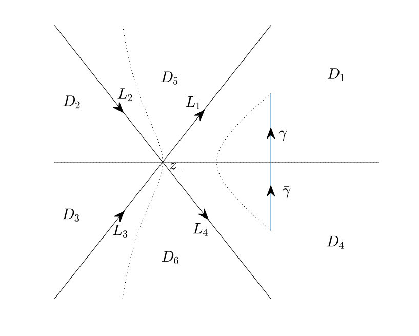 Figure 7
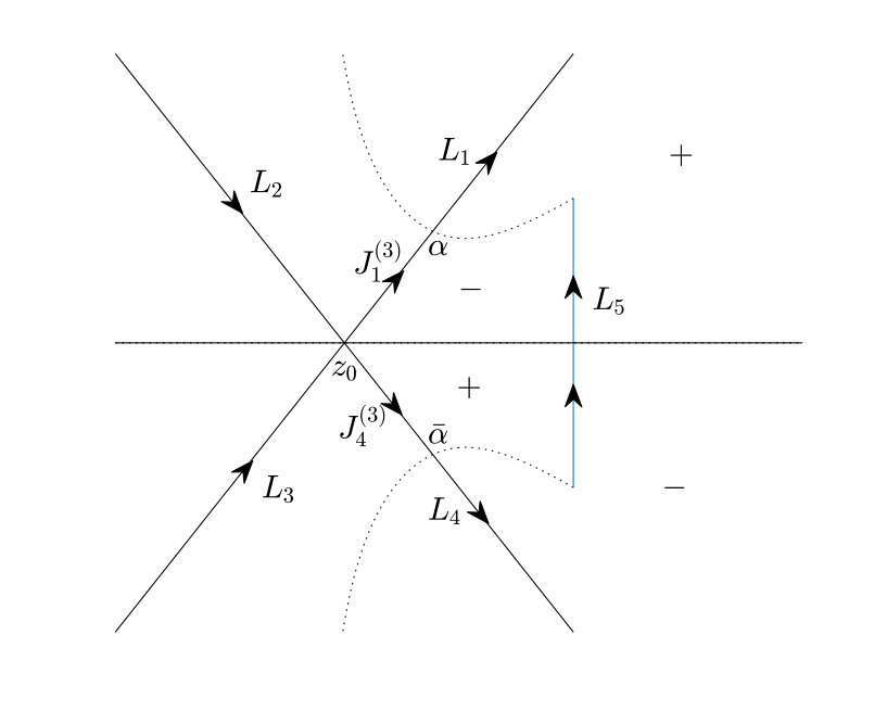 Figure 8
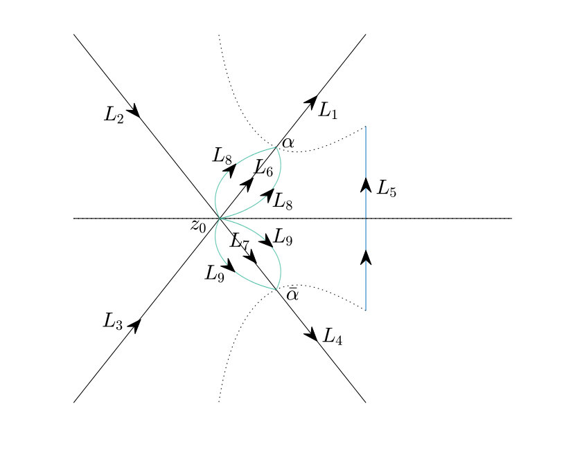 Figure 9
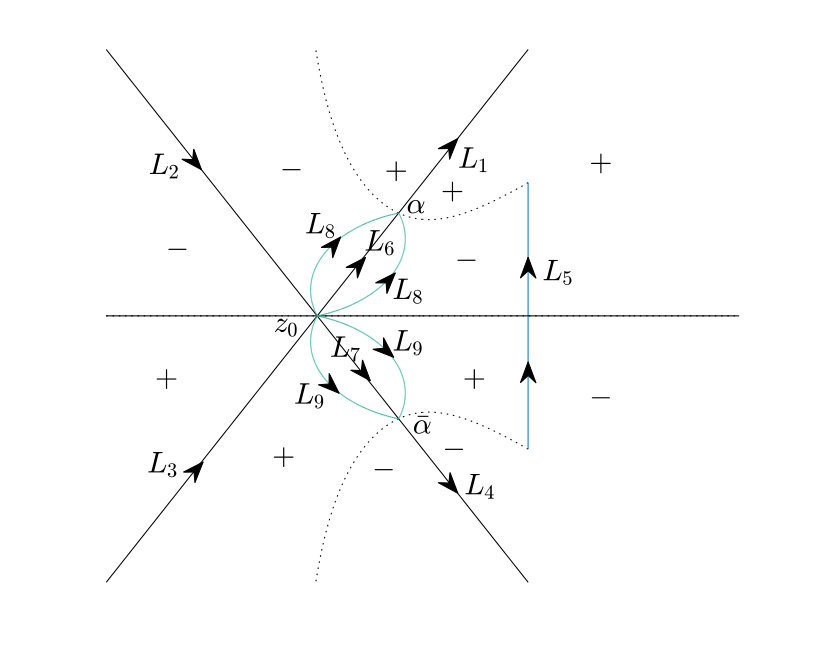 Figure 10
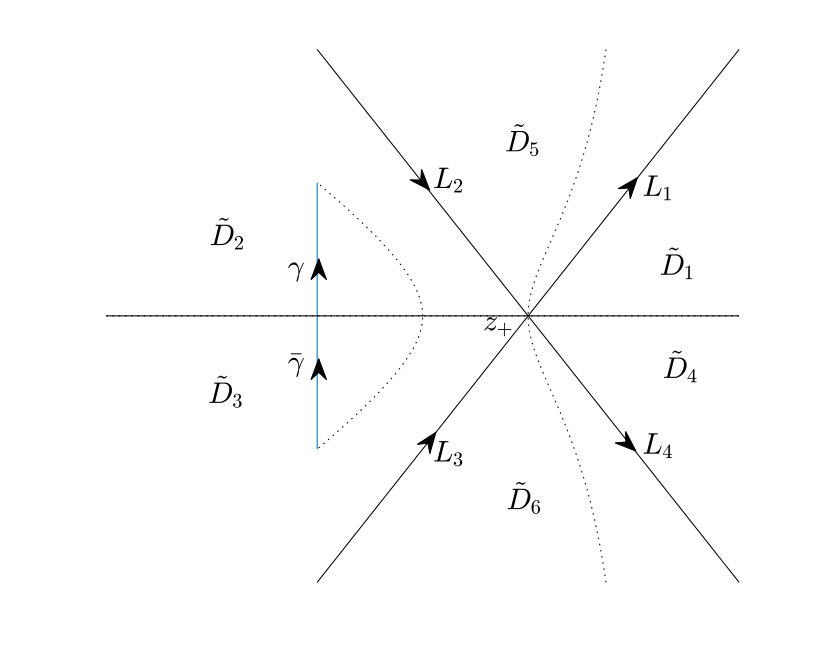 Figure 11
 Figure 1
Peer Reviews
No public reviews on file for this paper yet. If you reviewed it on a platform where reviews are public (OpenReview, ICLR, NeurIPS, ICML), you can paste yours below so the community can read it here.
Videos
No videos yet. Explain this paper in a talk, walkthrough, or lecture? Add one.
Taxonomy
TopicsNonlinear Waves and Solitons · Numerical methods for differential equations · Advanced Mathematical Physics Problems
The Gerdjikov-Ivanov type derivative nonlinear Schrödinger equation: Long-time
dynamics of nonzero boundary conditions
Boling Guoa, Nan Liu*b,****Corresponding author.
a**Institute of Applied Physics and Computational Mathematics, Beijing 100088, P.R. China
*b**The Graduate School of China Academy of Engineering Physics, Beijing 100088, P.R. China
††E-mail address: [email protected] (N. Liu).*
Abstract. We consider the Gerdjikov–Ivanov type derivative nonlinear Schrödinger equation
[TABLE]
on the line. The initial value is given and satisfies the symmetric, nonzero boundary conditions at infinity, that is, as , and . The goal of this paper is to study the asymptotic behavior of the solution of this initial-value problem as . The main tool is the asymptotic analysis of an associated matrix Riemann–Hilbert problem by using the steepest descent method and the so-called -function mechanism. We show that the solution of this initial value problem has a different asymptotic behavior in different regions of the -plane. In the regions and , the solution takes the form of a plane wave. In the region , the solution takes the form of a modulated elliptic wave.
Keywords: Gerdjikov–Ivanov type derivative nonlinear Schrödinger equation; Riemann–Hilbert problem; Long-time asymptotics; Nonlinear steepest descent method.
1 Introduction
The celebrated nonlinear Schrödinger (NLS) equation has been recognized as a ubiquitous mathematical model among many integrable systems, which governs weakly nonlinear and dispersive wave packets in one-dimensional physical systems. It plays an important role in nonlinear optics [15], water waves [3], and Bose–Einstein condensates [29]. Another integrable system of NLS type, the derivative-type NLS equation
[TABLE]
is derived by Gerdjikov–Ivanov [20], which is called the GI equation. Here and below, the bar refers to the complex conjugate. The GI equation can be regarded as an extension of the NLS when certain higher-order nonlinear effects are taken into account. In recent years, there has been much work on the GI equation, such as its Darboux transformation and Hamiltonian structures [16, 17], the algebra-geometric solutions [11], the rogue wave and breather solution [35]. Particularly, the long-time asymptotic behavior of solution to the GI equation (1.1) was established in [34, 31] by using the nonlinear steepest descent method.
In particular, via the transformation , equation (1.1) is trivially converted into
[TABLE]
Our purpose in the present work is devoted to the study of the long-time asymptotics of equation (1.2) on the line with symmetric, nonzero boundary conditions at infinity, that is,
[TABLE]
Hereafter, are complex constants and . This form of equation (1.2) has the advantage that the solutions of (1.2) which satisfy (1.3) are asymptotically time independent as The problems with nonzero boundary conditions at infinity of the kind (1.3) have already been studied. For example, the inverse scattering transform (IST) and the long-time asymptotics for the focusing NLS equation with nonzero boundary conditions at infinity were developed recently in [5] and [7], respectively. Furthermore, for the multi-component case, the initial value problem for the focusing Manakov system with nonzero boundary conditions at infinity is solved in [27] by developing an appropriate IST. The three-component defocusing NLS equation with nonzero boundary conditions was analyzed in [6] by the theory of IST. On the other hand, for the asymmetric non-zero boundary conditions (i.e., when the limiting values of the solution at space infinities have different non-zero moduli), the IST for the focusing and defocusing NLS equation were formulated in [14] and [4], respectively.
Our present work was motivated by the long-time asymptotic analysis for the focusing NLS equation developed in [7]. Our goal here is to compute the long-time asymptotics for the GI-type derivative NLS equation (1.2) with the initial value condition satisfied (1.3). The main tool is the asymptotic analysis of an associated matrix Riemann–Hilbert (RH) problem by using the steepest descent method and the so-called -function mechanism [12]. The well-known nonlinear steepest descent method introduced by Deift and Zhou in [13] provides a detailed rigorous proof to calculate the large-time asymptotic behaviors of the integrable nonlinear evolution equations. This approach has been successfully applied in determining asymptotic formulas for the initial value problems of a number of integrable systems associated with matrix sprectral problems including the mKdV equation [13], the KdV equation [21], the Hirota equation [24], the derivative NLS equation [30], the Fokas–Lenells equation [33] and the Kundu–Eckhaus equation [32]. For the matrix spectral problem, the large-time asymptotic behavior for the coupled NLS equations was obtained in [19] via nonlinear steepest descent. Moreover, there are also many beautiful results about the study of asymptotics of solutions of the initial value problems with shock-type oscillating initial data [10], nondecaying step-like initial data [9, 34, 26] and the initial-boundary value problems with -periodic boundary condition [8, 31] for various integrable equations. Recently, Lenells also has been derived some interesting asymptotic formulas for the solution of integrable equations on the half-line [28, 2] by using the steepest descent method. We also have done some meaningful work about determining the long-time asymptotics for integrable equations on the half-line, see [22, 23].
The organization of the paper is as follows. In Section 2, we formulate the main Riemann–Hilbert problem to solve the initial value problem for the GI-type derivative NLS equation (1.2) with nonzero boundary conditions. We then use this RH problem to compute the long-time asymptotic behavior of the solution in different regions of the -plane in Section 3.
2 The Riemann–Hilbert problem
In this section, we will use the approach proposed in [7] to formulate the main RH problem, which allows us to give a representation of the solution for the equation (1.2).
2.1 Eigenfunctions
The integrability of equation (1.2) follows from its Lax pair representation
[TABLE]
where
[TABLE]
is a vector or a matrix-valued function and is the spectral parameter, and
[TABLE]
Let and . It is straightforward to see that the eigenvector matrix of can be written as
[TABLE]
while the corresponding eigenvalues are defined by
[TABLE]
The branch cut for is taken along the segment
[TABLE]
where
On the other hand, one obtains that , we seek simultaneous solution of Lax pair (2.1) such that
[TABLE]
where
[TABLE]
We also find that for any , remain bounded as if and only if . The contour can be reduced to the contour in the -plane as shown in Fig. 1. Introducing a new eigenfunction by
[TABLE]
we obtain that
[TABLE]
Using the method of variation of parameters, we get the following Volterra integral equations for
[TABLE]
where and . Assuming , and , where
[TABLE]
the analysis of the Neumann series for the integral equations (2.12) and (2.13) allows one to prove existence and uniqueness of the eigenfunctions for all (the detailed proof can be founded [4, 5]). We denote by and the columns of . Then we have the following lemma.
Lemma 2.1
For all , the matrices have the following properties:
(i) The determinants of satisfy
[TABLE]
(ii) and are analytic in , and as
(iii) and are analytic in , and as
(iv) Symmetry:
[TABLE]
(v) Moreover,
[TABLE]
where
[TABLE]
Remark 2.1
The definition (2.6) of implies that is nonzero and nonsingular for all . The symmetry relations (2.15) and (2.16) can be proved easily due to the symmetries of the matrix :
[TABLE]
The large asymptotics of can be obtained from the -part of Lax pair (2.1) and (2.10) as well as the asymptotics of , that is, as .
Moreover, any two solutions of (2.1) are related, thus we define the spectral matrix by
[TABLE]
In particular, it follows from (2.14) that
[TABLE]
Due to the symmetry relation (2.15), the matrix-valued spectral functions can be defined in terms of two scalar spectral functions, and by
[TABLE]
where and indicate the Schwartz conjugates. Meanwhile, by the symmetry relation (2.16), one can infer that
[TABLE]
Finally, equations (2.10), (2.17) and (2.19) imply
[TABLE]
where wr denotes the Wronskian determinant. Thus, we can find that is analytic in .
The jump discontinuity of across induces a corresponding jump for the eigenfunctions and scattering data.
Lemma 2.2
The columns of fundamental solutions and scattering data , satisfy the following jump conditions across :
[TABLE]
and
[TABLE]
**Proof.**It is noted that the pairs and are both fundamental sets of solutions of -part Lax pair (2.1). Thus, the limit satisfies
[TABLE]
where are independent of . Letting on both side of above equation, we get from (2.5) and (2.8) that
[TABLE]
which yields the first relation of (2.25). The others follow the similar arguments. Combining (2.21) with (2.25), (2.23), we can easily obtain (2.27).
2.2 The Riemann–Hilbert problem and the solution of the Cauchy problem
The scattering relation (2.17) can be rewritten in the form of conjugation of boundary values of a piecewise analytic matrix-valued function on a contour in the complex -plane. The final form is
[TABLE]
where denote the boundary values of according to a chosen orientation of , see Fig. 1. Indeed, define the matrix as follows:
[TABLE]
where the dependence on the variables , , on the right-hand side has been suppressed for brevity. Then the boundary values relative to are related by (2.28) with the jump matrix is given by
[TABLE]
where
[TABLE]
We note that the jump of across is obtained according to the jump conditions in Lemma 2.2. Finally, it follows from Lemma 2.1 and the relationship (2.29) between and , it can be shown that admits the following large asymptotic expansion
[TABLE]
Thus, the solution of the GI-type derivative NLS equation (1.2) can be expressed in terms of the solution of the basic RH problem as follows:
[TABLE]
where is the solution of the following RH problem:
Suppose that for . Determine a matrix-valued function such that
is a sectionally meromorphic function in ;
satisfies the jump condition in (2.28) with the jump matrix given by (2.30);
has the following asymptotics:
[TABLE]
Although it is possible to perform this analysis directly in the complex -plane, the symmetry of the spectral functions in (2.20) suggest that it is convenient to introduce a new spectral variable by . This change of spectral parameter appeared already in [25] and was further employed in [2, 34]. One advantage of working with is that we can more easily analyze the signature table of the real part for the new phase function in order to find the long-time asymptotics.
The symmetry relation (2.16) implies that the solution obeys the symmetry
[TABLE]
Hence, letting , we can define by the equation
[TABLE]
The factor is included in (2.36) in order to make the right-hand side an even function of and acts on a matrix by ; the matrix involving is included to ensure that as . We define the new spectral function by
[TABLE]
Then the Riemann–Hilbert problem for can be rewritten in terms of as
[TABLE]
with the normalization condition
[TABLE]
where
[TABLE]
and
[TABLE]
In terms of , (2.33) can be expressed as
[TABLE]
3 The long-time asymptotics
In this section, we compute the long-time asymptotic behavior of the solution of the GI-type derivative NLS equation (1.2), as obtained by equation (2.43) by using the Deift-Zhou nonlinear steepest descent method to perform the asymptotic analysis of oscillating RH problems [7, 13, 8, 9, 10]. The key point of this method is the choice of contour deformations, which depends crucially on the sign structure of the quantity Re. We note that
[TABLE]
Thus, we get
[TABLE]
which implies that has two stationary points
[TABLE]
Letting , we have
[TABLE]
Hence, according to
[TABLE]
we can find the curves of the sets . In fact, the sign structure of Re(i in the complex -plane is shown in Fig. 2.
Remark 3.1
It is noted that , that is, or , the function has two real stationary points. We will show that this sectors of the -plane correspond to plane wave regions, whereas the sectors where correspond to modulated elliptic wave regions.
3.1 The plane wave region I:
For , that is, , has two real stationary points given by (3.3). This implies that one can introduce a complex-valued function to transform the original RH problem for to the RH problem for the new function by
[TABLE]
where
[TABLE]
Lemma 3.1
The function has the following properties:
(i) satisfies the following jump condition across the real axis oriented in Fig. 1:
[TABLE]
(ii) As , satisfies the asymptotic formula
[TABLE]
(iii) and are bounded and analytic functions of with continuous boundary values on .
(iv) obeys the symmetry
[TABLE]
Then satisfies the jump condition
[TABLE]
where the jump matrix is given by
[TABLE]
The new jump matrix can be analytically extended from . This leads to the next transformation:
[TABLE]
where is defined by
[TABLE]
The domains are shown on Fig. 3. Then the new function solves the following equivalent RH problem:
[TABLE]
where the curves can be chosen freely, only respecting that they pass through , do not cross , go to , and lie entirely in domains with the appropriate sign of Re, and the jump matrix is given by
[TABLE]
We have used the jump condition
[TABLE]
for across to derive the jump matrix .
The next deformation is aim to remove the function from the jump matrices (3.11) so that the jumps along the contours eventually tend to the identity matrix as . This can be accomplished by letting
[TABLE]
where is defined by
[TABLE]
Then it follows that satisfies the following jump conditions
[TABLE]
and the jump matrix is given by
[TABLE]
Obviously, for , , the jump matrix decays to identity matrix as exponentially fast and uniformly outside any neighborhood of . In order to arrive at a RH problem whose jump matrix does not depend on , we introduce a factorization involving a scalar function to be defined:
[TABLE]
in such a way that the boundary values of along the two sides of satisfy
[TABLE]
Indeed, once (3.16) is satisfied, one can absorb the diagonal factors into a new piecewise analytic function whose jump across is only the constant middle factor in (3.16).
The function can be determined explicitly as follows. Dividing condition (3.17) by , we deduce that
[TABLE]
and
[TABLE]
Plemelj’s formula [1] then yields in the explicit form
[TABLE]
As , we find that
[TABLE]
where
[TABLE]
The factorization (3.16) suggests the final transformation
[TABLE]
Then we have
[TABLE]
for (see Fig. 3). Meanwhile, the jump matrix satisfies:
for , jump matrix is a constant
[TABLE]
for , jump matrix decays to the identity
[TABLE]
uniformly outside any neighborhood of .
Finally, one can write in the form
[TABLE]
where solves the model problem:
[TABLE]
with constant jump matrix
[TABLE]
and
[TABLE]
The last estimate (3.26) can be justified by considering the parametrix associated with the RH problem for , see [10, 7]. The error of order comes from the contribution of the jump near .
Define
[TABLE]
Then, we have
[TABLE]
on , and admits the large- expansion
[TABLE]
As for the model RH problem, its solution thus can be given explicitly in terms of :
[TABLE]
Then, going back to the determination of in terms of the solution of the basic RH problem, we have
[TABLE]
Taking into account that , and , we arrive at the following theorem.
Theorem 3.1
In the region , as , the asymptotics of the solution of the initial value problem for the GI-type derivative NLS equation (1.2) takes the form of a plane wave:
[TABLE]
where is defined by (3.21).
Remark 3.2
If we let , then . Thus, we get , and then the asymptotic formulae (3.30) reduces to . This is correspondence to our initial condition up to a phase shift as .
3.2 The modulated elliptic wave region I:
In this subsection we compute the leading-order long-time asymptotics of the solution of the GI-type derivative NLS equation (1.2) in the region . Recalling the sign structure of Re in this region depicted in Fig. 2, the main difference is the absence of real stationary points compared with the plane wave region I. This implies that it is not possible anymore to use the previous factorizations and deformations to lift the contours off the real -axis in such a way that the corresponding jump matrices remain bounded as . Therefore, developing and extending the ideas used in [10, 7], we introduce a new -function appropriate for the region under consideration, which has a new real stationary point .
Let us perform the same transformations
[TABLE]
as in Subsection 3.1 for the plane wave region I but with characterized by instead of the point , that is,
[TABLE]
In this subsection, we will use the notation to denote for simplicity. It then follows that the function is analytic in and satisfies the jump conditions
[TABLE]
with the normalization condition
[TABLE]
The jump contours is shown in Fig. 4, the jump matrices are given by equations (3.15) and defined by (3.31).
We now encounter a new phenomenon that is not present in the plane wave region I, namely, the jumps and grow exponentially with along the segments and as shown in Fig. 4, respectively. In order to overcome this difficulty, we employ the new factorizations for these jumps:
[TABLE]
where
[TABLE]
These factorizations allow for the deformation of the segments and of Fig. 4 into the contours shown in Fig. 5, where denote the restriction of to the contours labeled by in Fig. 5. We next employ the -function mechanism, more precisely, let
[TABLE]
for a function that is required to be analytic in . In fact, it is more convenient to consider the function define by
[TABLE]
Then, one can infer that is analytic in and has jump discontinuities across and . Furthermore, the jump conditions of function read
[TABLE]
We next turn to determine , and such that all these jump matrices remain bounded as by using the methods in [7, 9]. Let
[TABLE]
Define function with branch cuts and by
[TABLE]
We fix the branch cut to be oriented upwards, then for . The gives rise to a genus-1 Riemann surface with sheets , and a basis of cycles defined as follows: the b-cycle is a closed, anticlockwise contour around the branch cut that remains entirely on the first sheet of the Riemann surface; the a-cycle consists of an anticlockwise contour that starts on the left side of , then goes from the right while on the first sheet , and finally returns to the starting point via the second sheet .
Next, we let be given by the sum of two Abelian integrals:
[TABLE]
where the Abelian differential is defined by
[TABLE]
and , are to be determined. We can also write the Abelian differential in the following form:
[TABLE]
then, we have
[TABLE]
We then have
[TABLE]
In order to preserve the sign structure in the transition from to , we require that has the same large- behavior as the function :
[TABLE]
This condition implies:
[TABLE]
Observe that
[TABLE]
Thus, the large- asymptotics of can be specified as
[TABLE]
where
[TABLE]
Moreover, combining (3.39) and (3.41), we get
[TABLE]
It thus remains to determine . We do so by analyzing the behavior of near . In a neighborhood of , it follows from (3.38) that
[TABLE]
Thus, we obtain the expansion
[TABLE]
where
[TABLE]
In order to obtain the desired sign structure as shown in Fig. 6, the leading-order term of the expansion of Re near should be of . Thus, we must have Im. Hence, we get
[TABLE]
According to the discussion in [7], one can rewrite the condition (3.46) as the following forms
[TABLE]
Finally, substituting (3.44) into (3.47), we find
[TABLE]
It is enough to determine the from equation (3.48), and hence , function .
Lemma 3.2
For all , the integral equation (3.48) admits a unique solution .
**Proof.**The strategy of the proof follows from [7, 9]. Let
[TABLE]
Then, equation (3.48) turns into
[TABLE]
which is considered for . It is easy to check that , . Moreover, for . Therefore, by the implicit function theorem, (3.49) determines a unique function for any such that and . That is, for any there exists a unique solution of the integral equation (3.48) with .
We have now specified a -function which has appropriate signature table as in Fig. 6. Moreover, across the branch cuts and , satisfies the following jump conditions
[TABLE]
where the real constant is defined by
[TABLE]
In the following, we continue to deform the RH problem. By the jumps (3.50) of , we infer that the jump matrices of can be rewritten as
[TABLE]
where for we denote by the jump associated with the contour . Furthermore, the normalization condition of is
[TABLE]
Recalling (3.36), (3.42), (3.43) and
[TABLE]
we find that the real constant involved in the (3.35) is equal to
[TABLE]
Our final task is to eliminate the dependence on from the jump matrices across the branch cuts for . To achieve this goal, we let
[TABLE]
The function is analytic in with jumps
[TABLE]
with the function defined by (3.31) and the real constant determined by
[TABLE]
It follows from the Plemelj’s formulae that
[TABLE]
The definition (3.56) of ensures that
[TABLE]
where the real constant is given by
[TABLE]
Finally, we can obtain the following RH problem for :
[TABLE]
with the jump matrices given by
[TABLE]
and the normalization condition
[TABLE]
In other words, for the jump matrix , we have
[TABLE]
where and
[TABLE]
Thus, we arrive at the following model problem RHmod:
[TABLE]
The solution of RHmod approximates as follows (see the parametrix analysis in [10])
[TABLE]
The model RH problem (3.62) can be solved in terms of elliptic theta functions. Let us consider the Abelian differential
[TABLE]
which is normalized so that and has Riemann period defined by
[TABLE]
Note that . It can be shown that (see [18]). Define
[TABLE]
Then the following relations are valid:
[TABLE]
Next, we define a new function by
[TABLE]
which has the same jump discontinuity across both and , namely,
[TABLE]
and admits the large- asymptotic behavior
[TABLE]
The last ingredient is the theta function with :
[TABLE]
which has the following properties
[TABLE]
Now we define the matrix-valued function with entries:
[TABLE]
where
[TABLE]
Then the solution of the model RH problem (3.62) is given by
[TABLE]
Taking into account (3.35), (3.54) and (3.63), we get
[TABLE]
However, we have
[TABLE]
where
[TABLE]
Taking into account (3.53) and (3.58), we get the asymptotics of the solution in the region .
Theorem 3.2
In the region , the asymptotics of the solution of the initial value problem for the GI-type derivative NLS equation (1.2) takes, as , the form of a modulated elliptic wave:
[TABLE]
where the constants , , , , , and are given by the equations (3.44), (3.51), (3.56), (3.71), (3.68), (3.53) and (3.58), respectively.
3.3 The plane wave and modulated elliptic wave regions II
In the rest of the present paper, we devoted to discuss the long-time asymptotics of the solution of the initial value problem for GI-type derivative NLS equation (1.2) in the plane wave region II: and modulated elliptic wave region II: .
We first consider the region . In this case we first rescale the RH problem (2.38) for as follows, which is motivated by the ideas used in [7]. Let
[TABLE]
where
[TABLE]
Then, is analytic in and satisfies the following jump conditions
[TABLE]
with the normalization condition
[TABLE]
where
[TABLE]
and
[TABLE]
Then, we have
[TABLE]
As the discussions in plane wave region I, the first deformation for is
[TABLE]
where
[TABLE]
Then satisfies the following RH problem
[TABLE]
where the jump matrix is given by
[TABLE]
The next transformation is
[TABLE]
where is defined by
[TABLE]
and the domains are shown in Fig. 7. Then the function solves the following equivalent RH problem:
[TABLE]
where the contours are shown in Fig. 7 and the jump matrix is given by
[TABLE]
Then, performing the similar deformation and analysis as in Subsection 3.1, we can get a model RH problem which can be solved explicitly and obtain the long-time asymptotics for the solution . We just give the main results here.
Theorem 3.3
In the region , the asymptotics of the solution as of the initial value problem for the GI-type derivative NLS equation (1.2) takes the form of a plane wave:
[TABLE]
where is given by
[TABLE]
For the modulated elliptic wave region II: , the asymptotic analysis is entirely analogous to Subsection 3.2 after the rescaling the RH problem for as stated above. We omit the detailed computation here.
Acknowledgments.
This work was supported in part by the National Natural Science Foundation of China under grants 11731014, 11571254 and 11471099.
The reference list from the paper itself. Each links out to its DOI / PubMed record.
- 1[1] M.J. Ablowitz, A.S. Fokas, Complex Analysis: Introduction and Applications, 2nd ed. Cambridge University Press, Cambridge (2003).
- 2[2] L.K. Arruda, J. Lenells, Long-time asymptotics for the derivative nonlinear Schrödinger equation on the half-line, Nonlinearity 30 (2017) 4141–4172.
- 3[3] D.J. Benney, A.C. Newell, The propagation of nonlinear wave envelopes, Stud. Appl. Math. 46 (1967) 133–139.
- 4[4] G. Biondini, E. Fagerstrom, B. Prinari, Inverse scattering transform for the defocusing nonlinear Schrödinger equation with fully asymmetric non-zero boundary conditions, Phys. D 333 (2016) 117–136.
- 5[5] G. Biondini, G. Kovačič, Inverse scattering transform for the focusing nonlinear Schrödinger equation with nonzero boundary conditions. J. Math. Phys. 55 (2014) 031506.
- 6[6] G. Biondini, D. Kraus, B. Prinari, The three-component defocusing nonlinear Schröinger equation with nonzero boundary conditions, Comm. Math. Phys. 348 (2016) 475–533.
- 7[7] G. Biondini, D. Mantzavinos, Long-time asymptotics for the focusing nonlinear Schrödinger equation with nonzero boundary conditions at infinity and asymptotic stage of modulational instability, Comm. Pure Appl. Math. 70 (2017) 2300–2365.
- 8[8] A. Boutet de Monvel, A. Its, V. Kotlyarov, Long-time asymptotics for the focusing NLS equation with time-periodic boundary condition on the half-line, Comm. Math. Phys. 290 (2009) 479–522.