White dwarfs in the building blocks of the Galactic spheroid
Pim van Oirschot, Gijs Nelemans, Else Starkenburg, Silvia Toonen,, Amina Helmi, Simon Portegies Zwart

TL;DR
This study explores how the properties of galactic building blocks influence the halo white dwarf population and luminosity functions, revealing subtle differences linked to age and metallicity, but also highlighting observational challenges.
Contribution
It introduces a detailed modeling approach combining binary population synthesis with galaxy formation simulations to analyze halo white dwarf populations from different building blocks.
Findings
WDs from younger and/or metal-rich building blocks can be distinguished from others.
Halo WD luminosity functions are very similar across different building blocks.
IMF choice affects the fit to observed luminosity functions, with Kroupa or Salpeter performing slightly better.
Abstract
The galactic halo likely grew over time in part by assembling smaller galaxies, the so-called building blocks. We investigate if the properties of these building blocks are reflected in the halo white dwarf (WD) population in the Solar neighborhood. Furthermore, we compute the halo WD luminosity functions (WDLFs) for four major building blocks of five cosmologically motivated stellar haloes. We couple the SeBa binary population synthesis model to the Munich-Groningen semi-analytic galaxy formation model, applied to the high-resolution Aquarius dark matter simulations. Although the semi-analytic model assumes an instantaneous recycling approximation, we model the evolution of zero-age main sequence stars to WDs, taking age and metallicity variations of the population into account. Although the majority of halo stars is old and metal-poor and therefore the WDs in the different building…
Click any figure to enlarge with its caption.
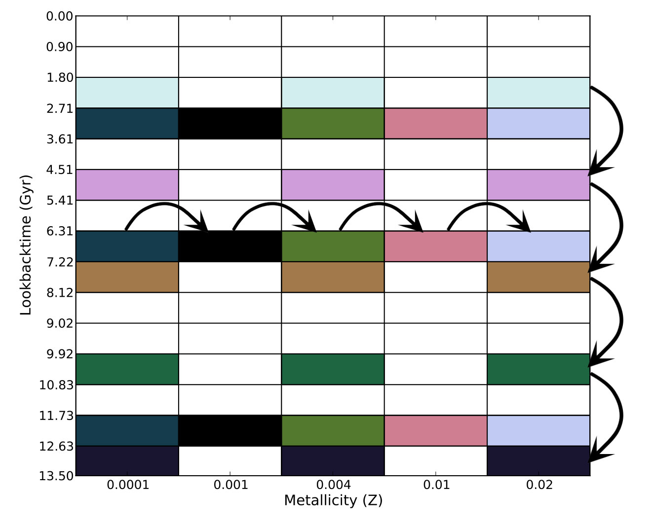 Figure 1
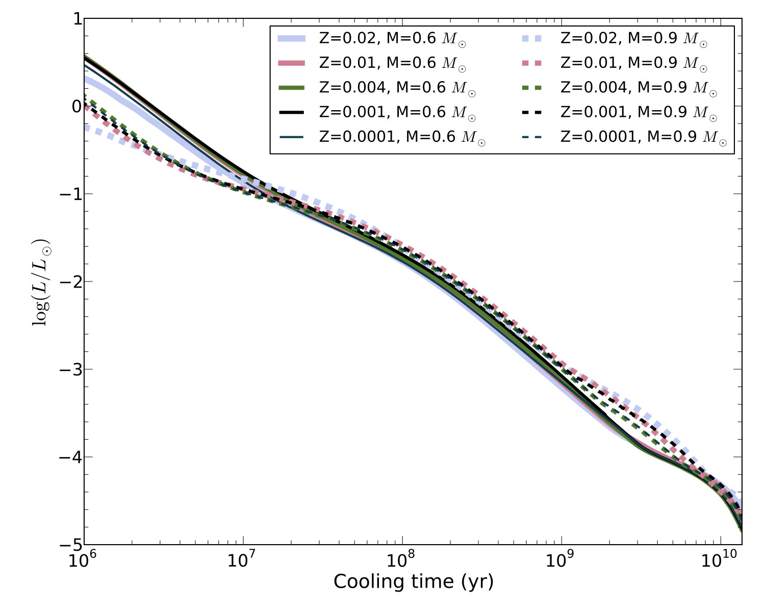 Figure 2
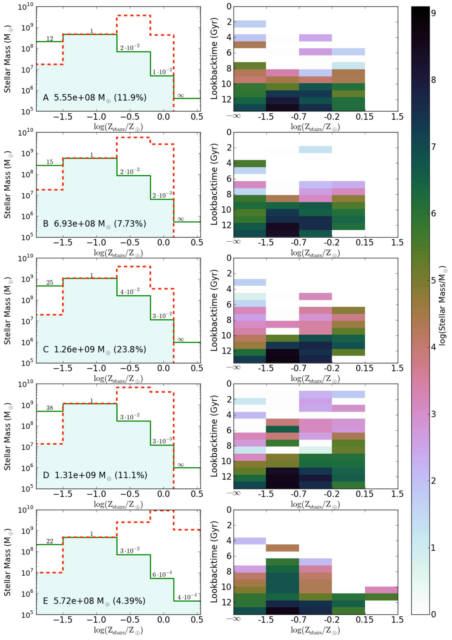 Figure 4
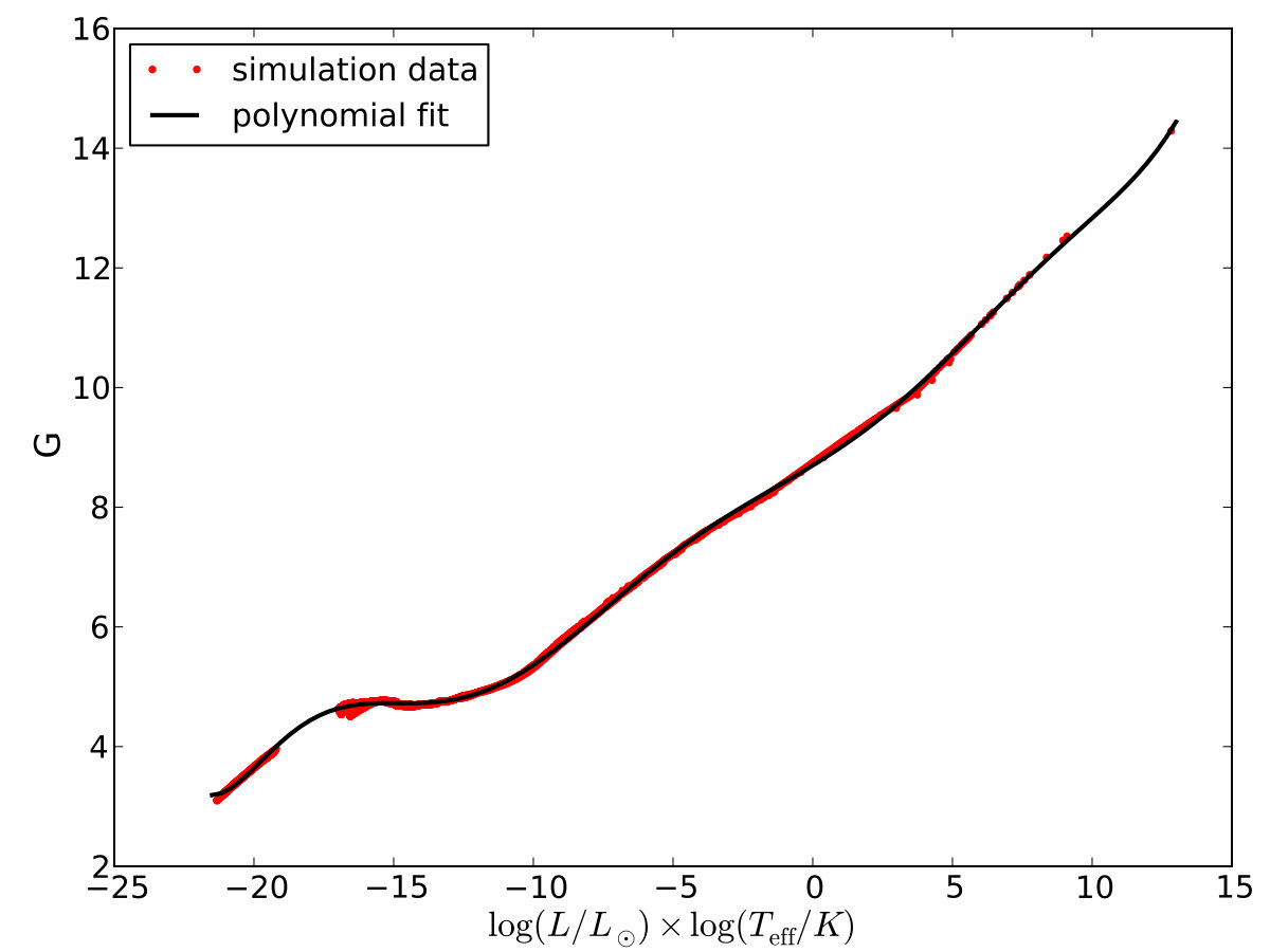 Figure 4
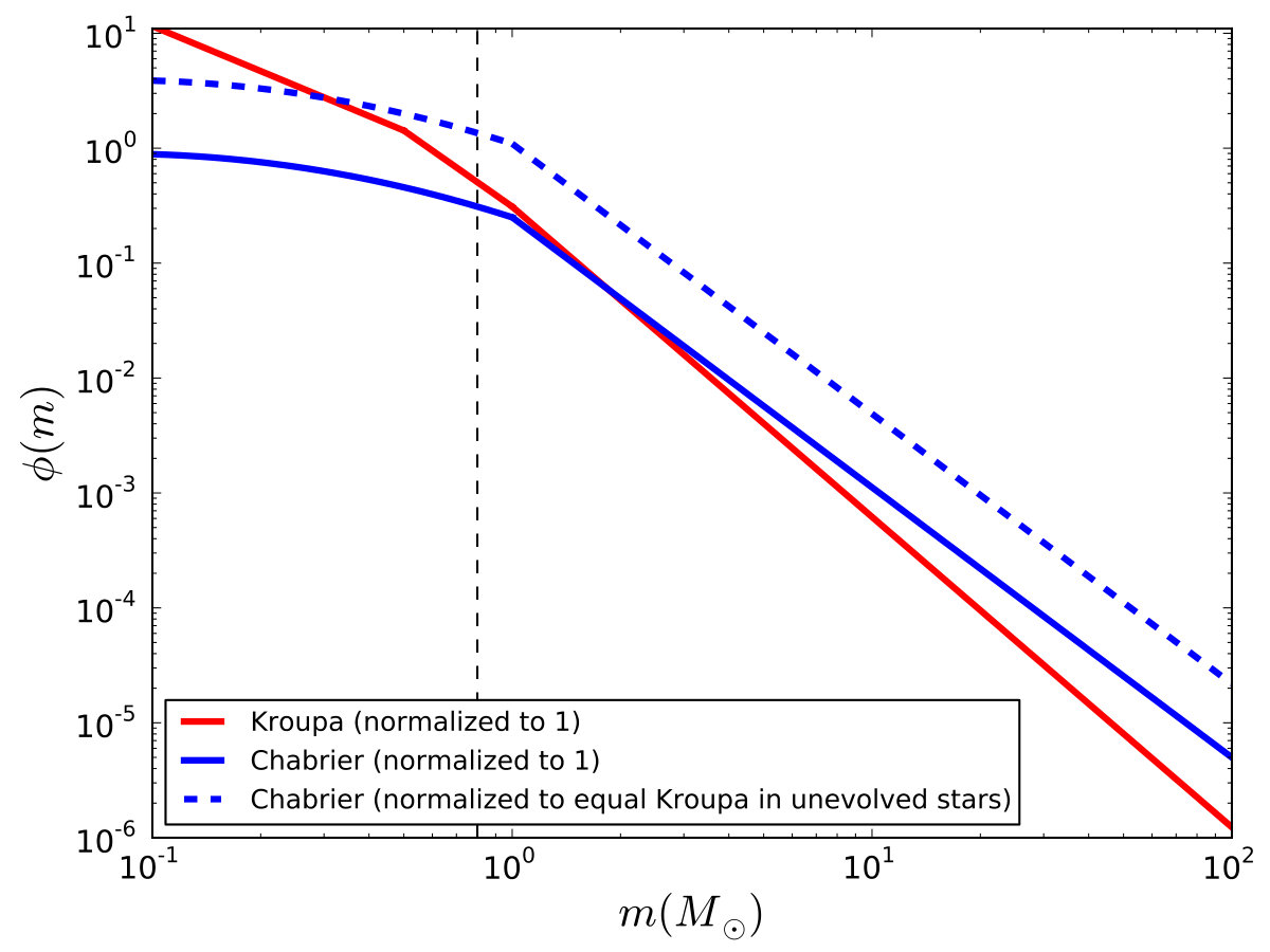 Figure 5
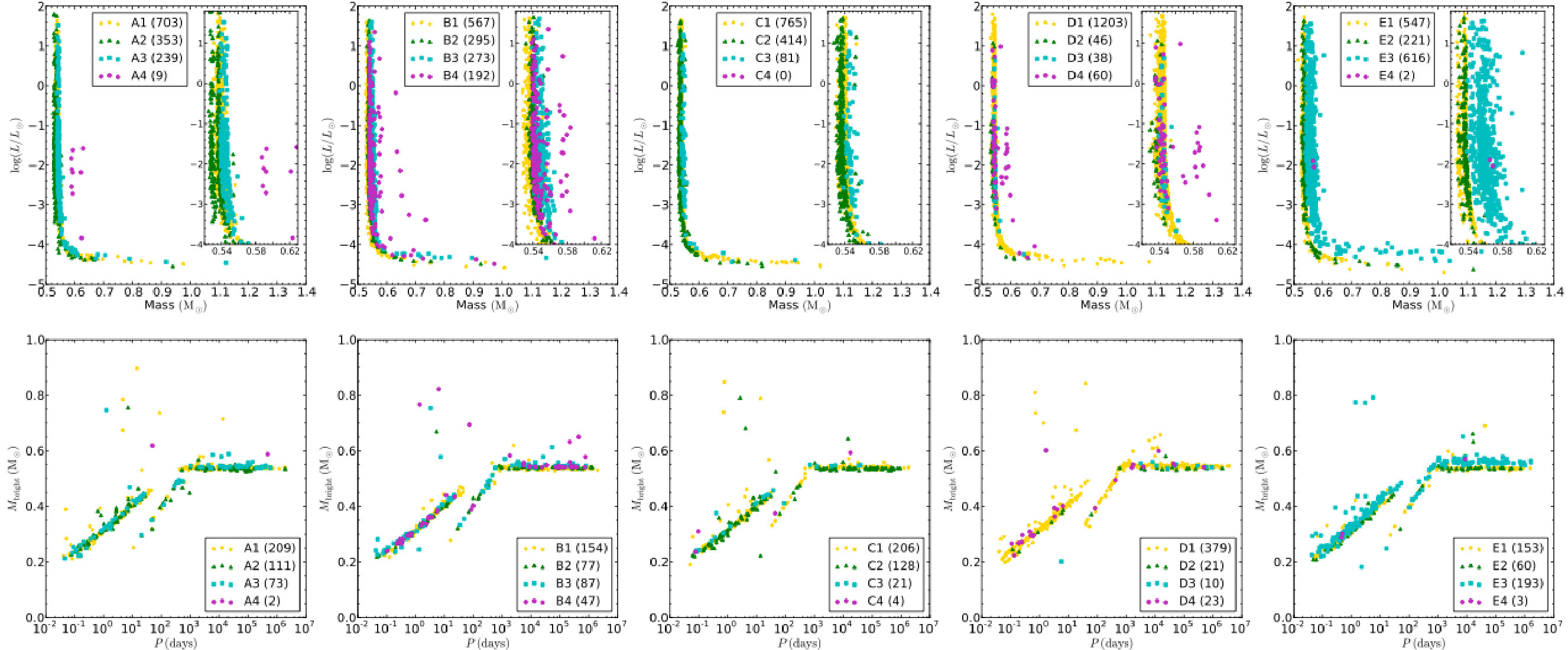 Figure 13
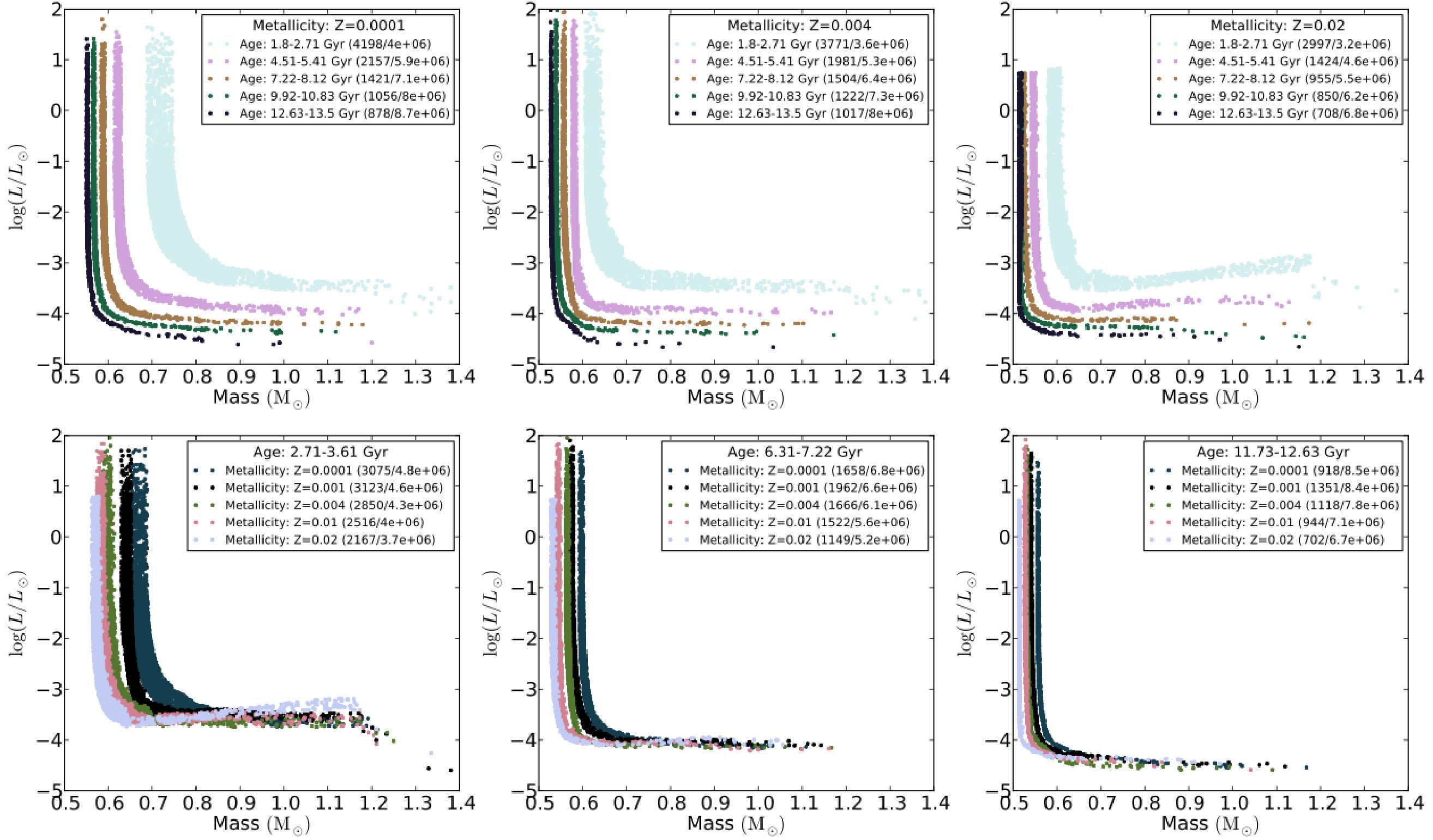 Figure 8
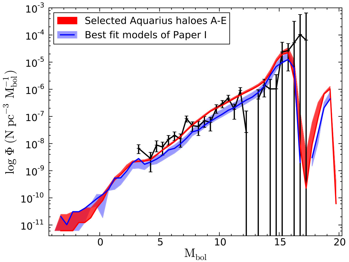 Figure 8
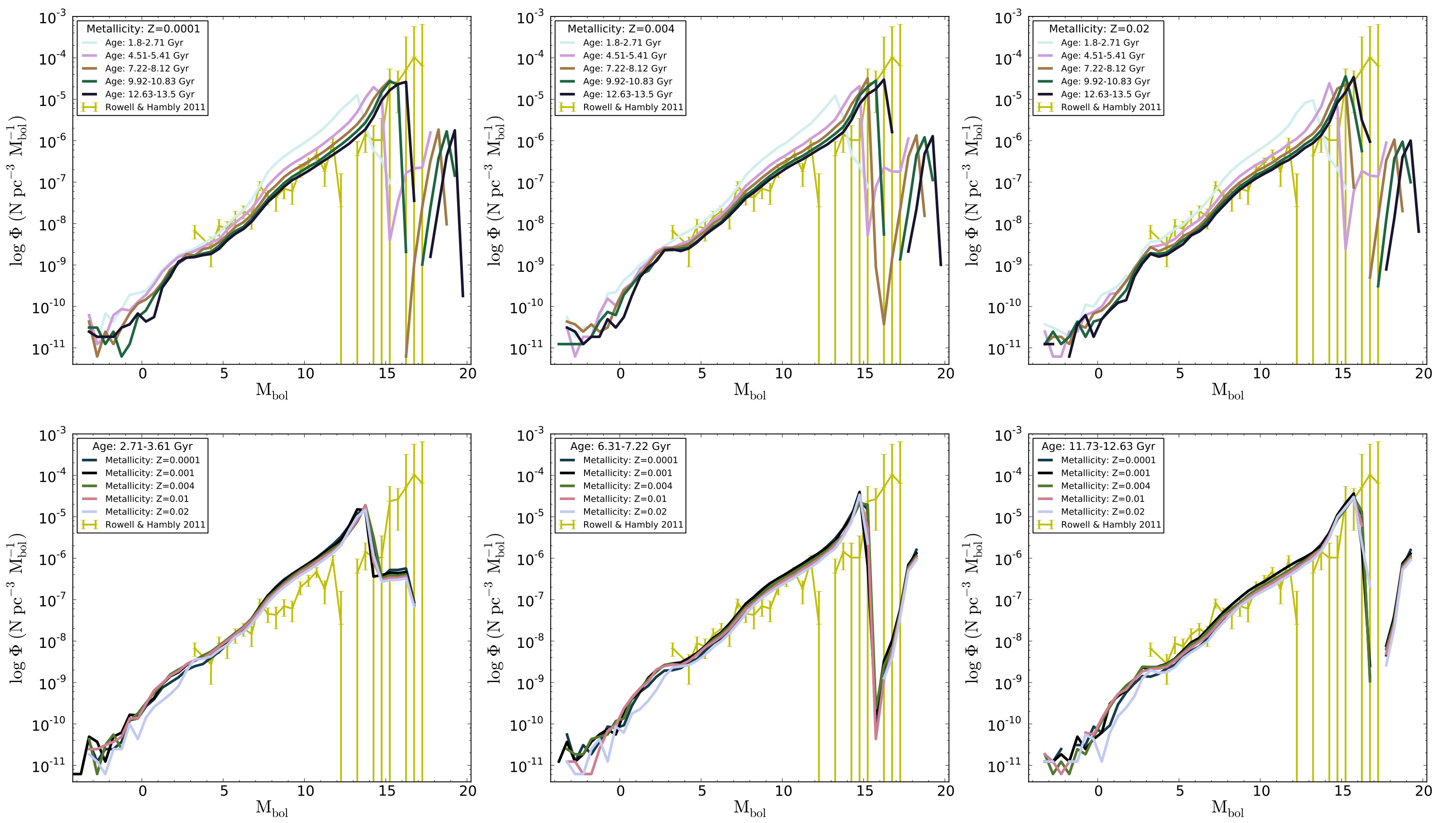 Figure 9
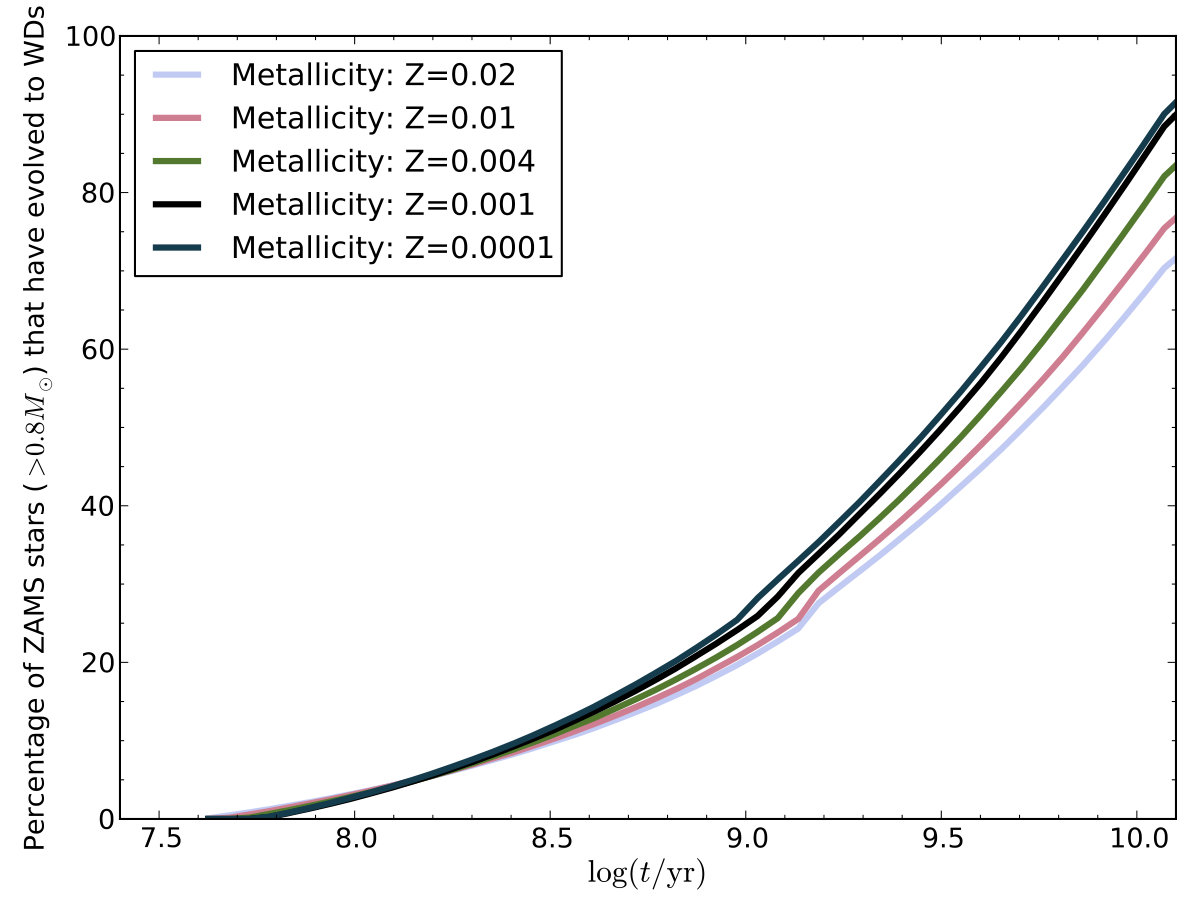 Figure 10
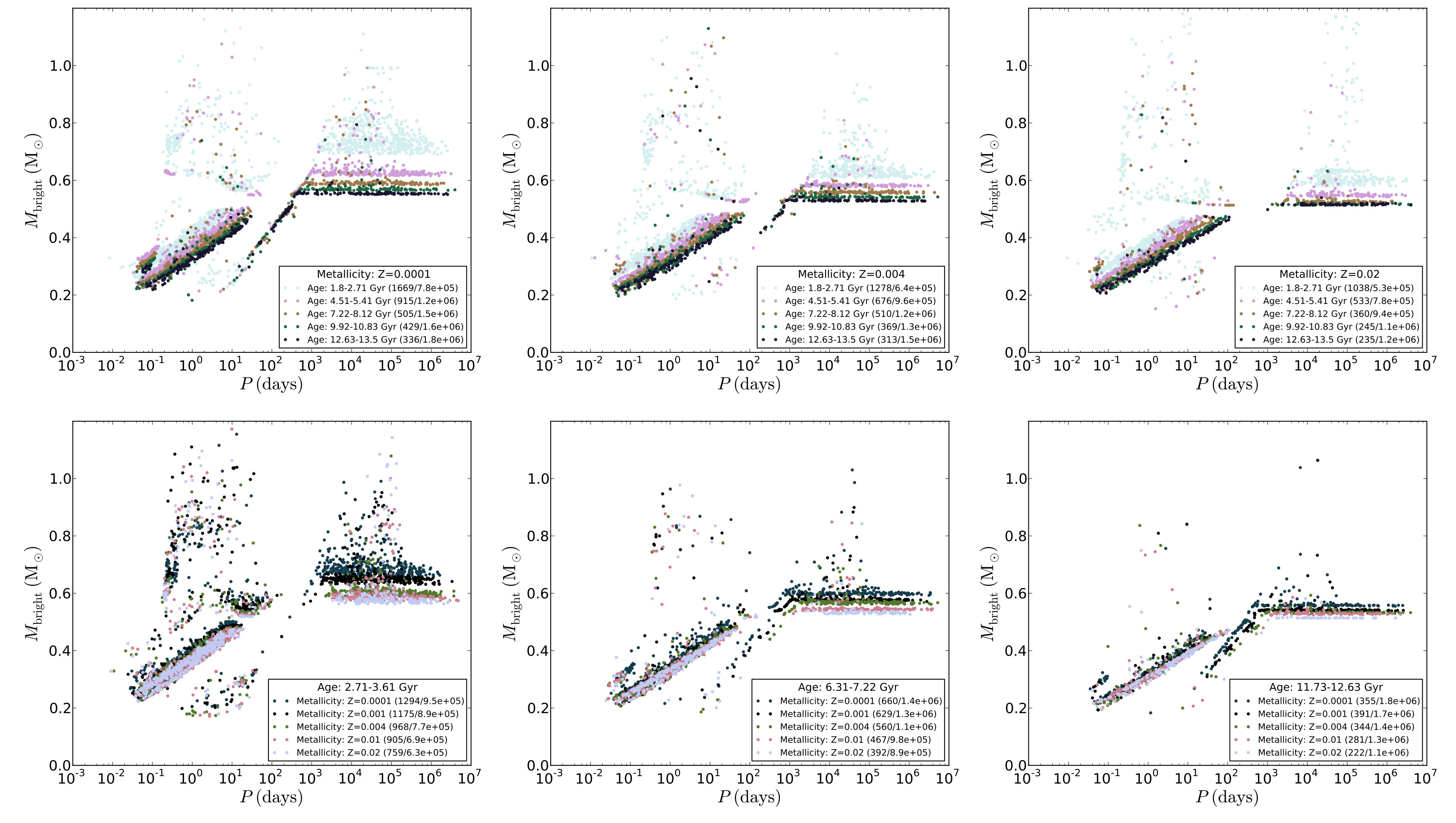 Figure 11
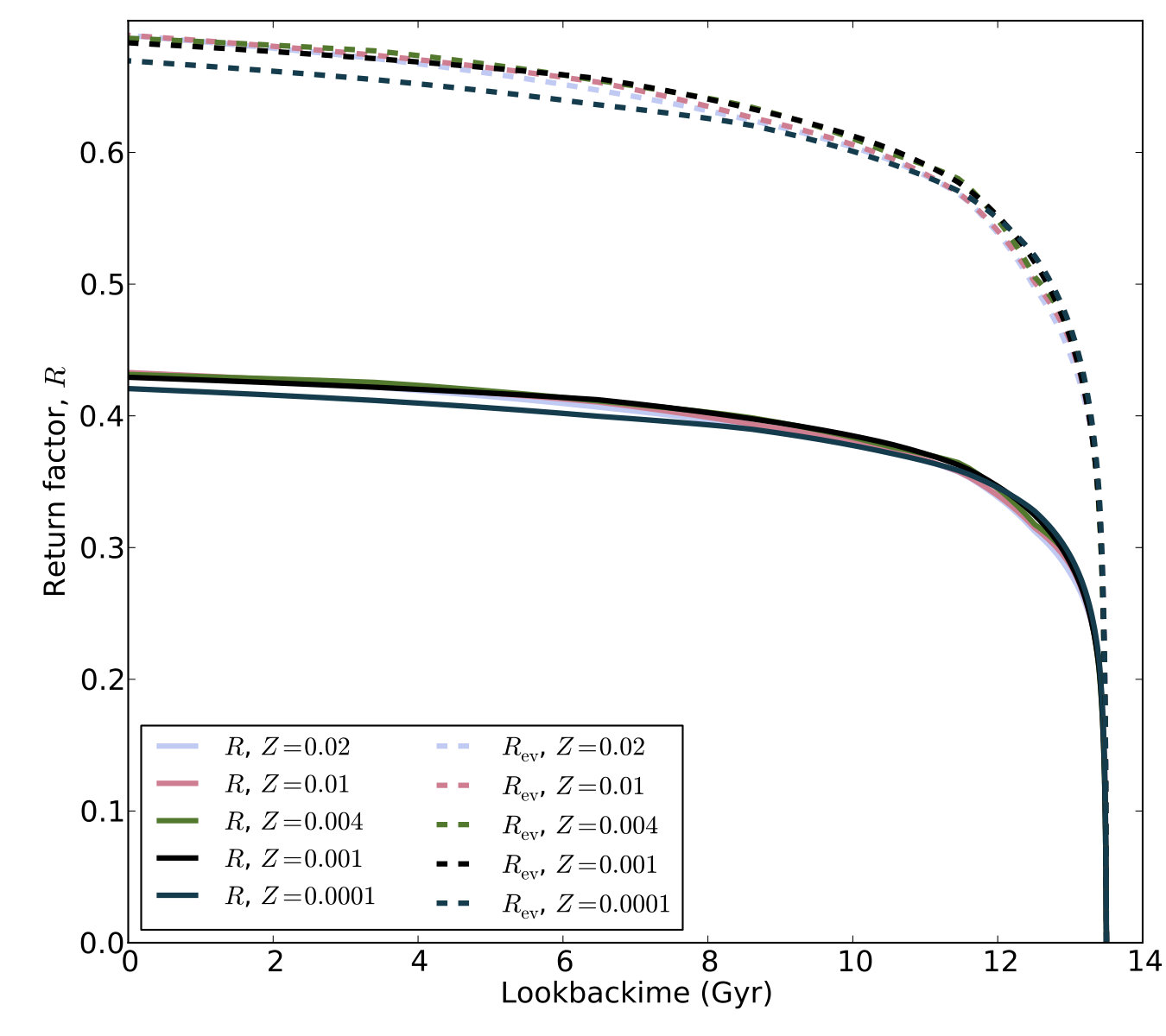 Figure 12
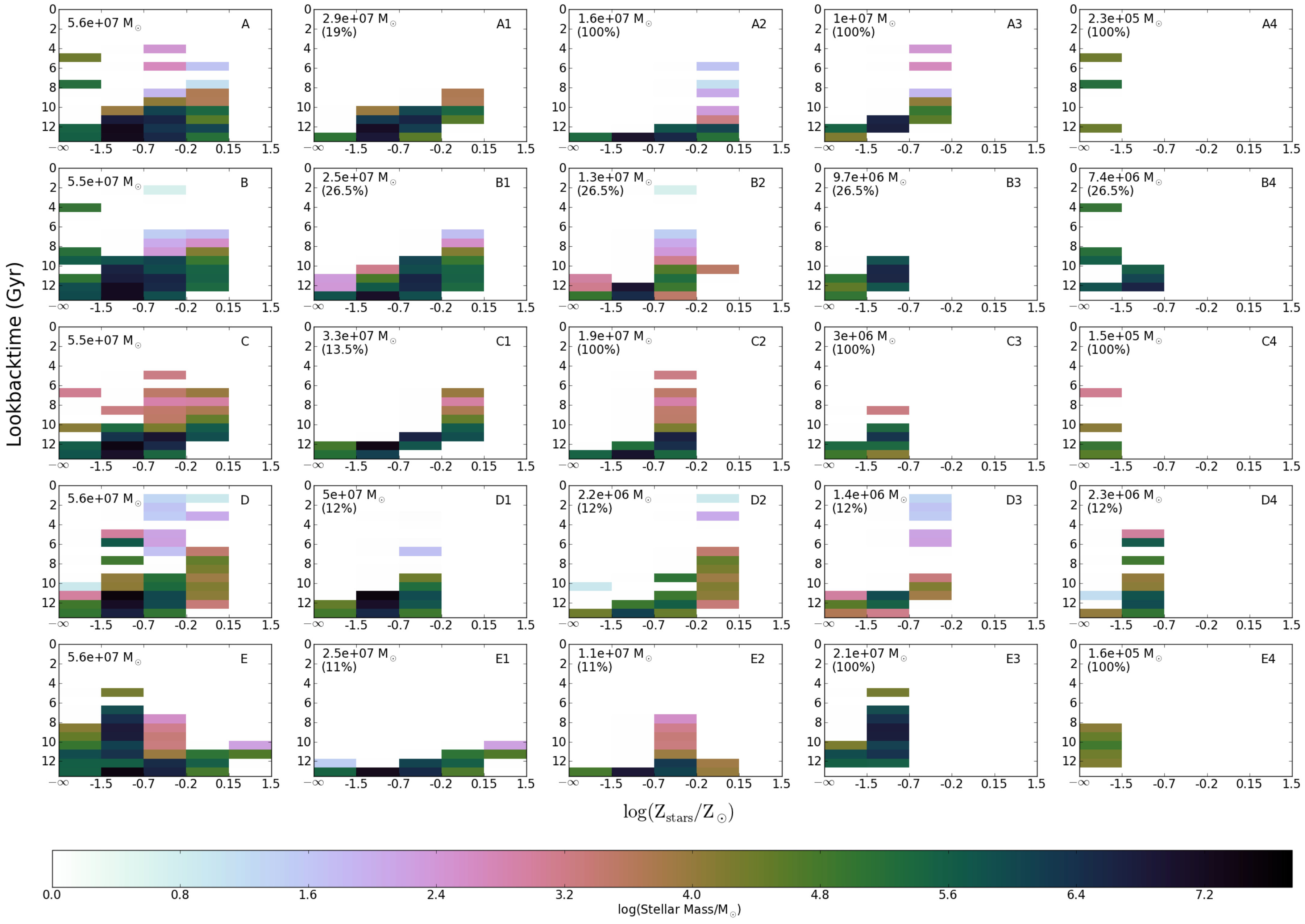 Figure 13
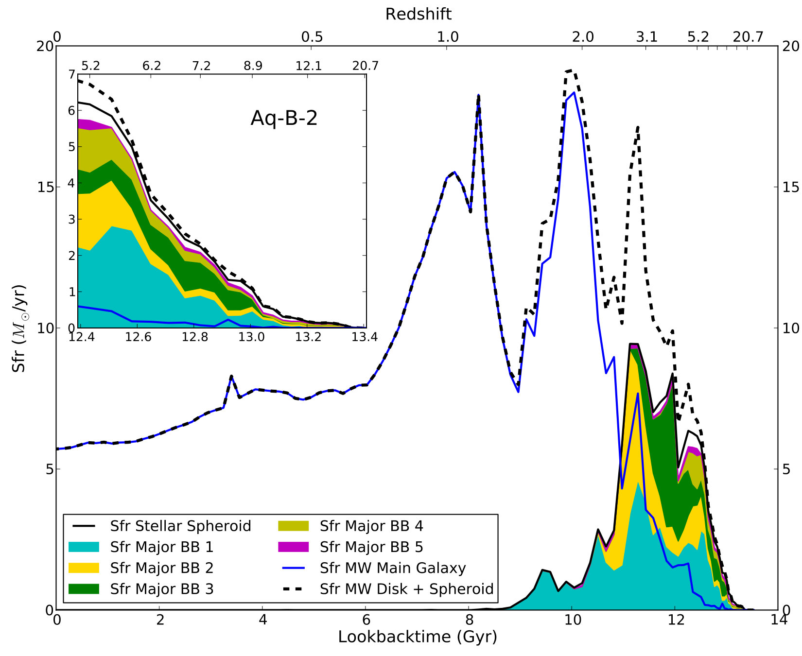 Figure 14
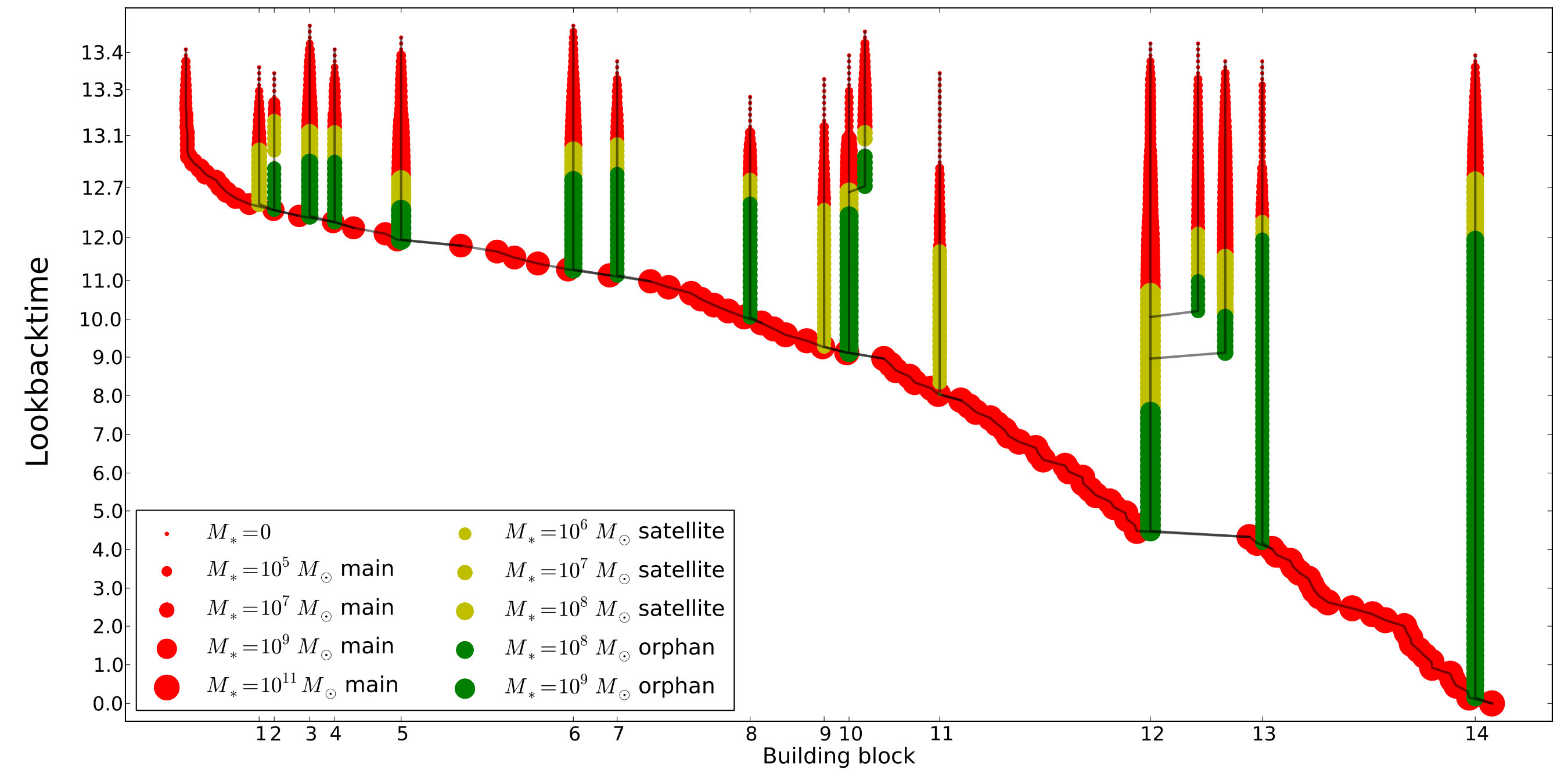 Figure 15
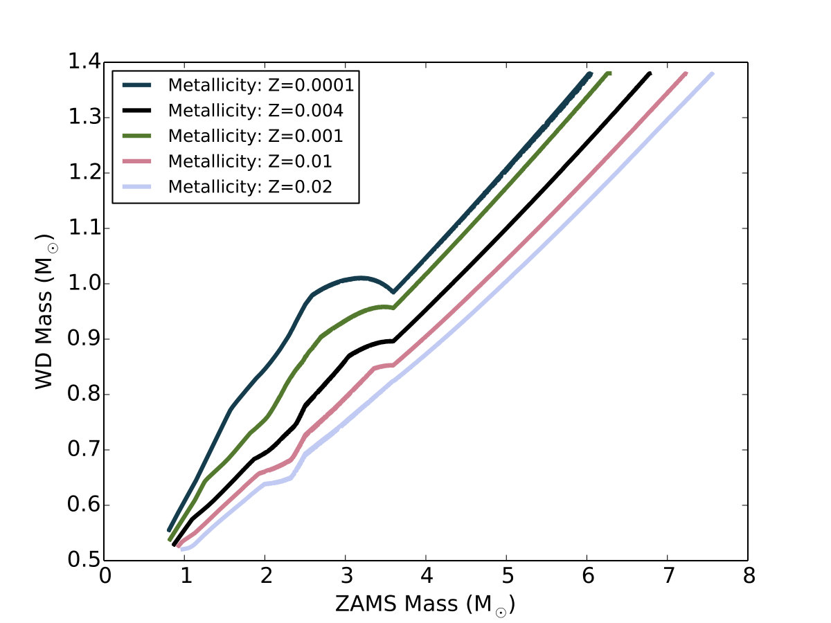 Figure 16
| =0.0001 | =0.001 | =0.004 | =0.01 | =0.02 | |
|---|---|---|---|---|---|
| He (S) | 0.144 | 0.161 | 0.148 | 0.146 | 0.142 |
| 0.509 | 0.496 | 0.487 | 0.481 | 0.476 | |
| CO (S) | 0.330 | 0.330 | 0.330 | 0.330 | 0.330 |
| 1.38 | 1.29 | 1.33 | 1.35 | 1.38 | |
| CO (L) | 0.520 | 0.505 | 0.503 | 0.525 | 0.54 |
| 0.826 | 0.863 | 0.817 | 0.934 | 1.20 |
Peer Reviews
No public reviews on file for this paper yet. If you reviewed it on a platform where reviews are public (OpenReview, ICLR, NeurIPS, ICML), you can paste yours below so the community can read it here.
Videos
No videos yet. Explain this paper in a talk, walkthrough, or lecture? Add one.
11institutetext: Department of Astrophysics/IMAPP, Radboud University, P.O. Box 9010, 6500 GL Nijmegen, The Netherlands 22institutetext: Institute for Astronomy, KU Leuven, Celestijnenlaan 200D, 3001 Leuven, Belgium 33institutetext: Leibniz-Institut für Astrophysik Potsdam, AIP, An der Sternwarte 16, D-14482 Potsdam, Germany 44institutetext: Leiden Observatory, Leiden University, P.O. Box 9513, 2300 RA Leiden, The Netherlands 55institutetext: Kapteyn Astronomical Institute, University of Groningen, P.O. Box 800, 9700 AV, Groningen, The Netherlands
White dwarfs in the building blocks of the Galactic spheroid
Pim van Oirschot 11 [email protected]
Gijs Nelemans 1122
Else Starkenburg 33
Silvia Toonen 44
Amina Helmi 55
Simon Portegies Zwart 44
(Received 9 Sep 2016 / Accepted 10 Sep 2016)
Abstract
*Aims. *The galactic halo likely grew over time in part by assembling smaller galaxies, the so-called building blocks. We investigate if the properties of these building blocks are reflected in the halo white dwarf (WD) population in the Solar neighborhood. Furthermore, we compute the halo WD luminosity functions (WDLFs) for four major building blocks of five cosmologically motivated stellar haloes. We compare the sum of these to the observed WDLF of the galactic halo, derived from selected halo WDs in the SuperCOSMOS Sky Survey, aiming to investigate if they match better than the WDLFs predicted by simpler models.
*Methods. * We couple the SeBa binary population synthesis model to the Munich-Groningen semi-analytic galaxy formation model, applied to the high-resolution Aquarius dark matter simulations. Although the semi-analytic model assumes an instantaneous recycling approximation, we model the evolution of zero-age main sequence stars to WDs, taking age and metallicity variations of the population into account. To be consistent with the observed stellar halo mass density in the Solar neighborhood (), we simulate the mass in WDs corresponding to this density, assuming a Chabrier initial mass function (IMF) and a binary fraction of 50%. We also normalize our WDLFs to .
*Results. *Although the majority of halo stars is old and metal-poor and therefore the WDs in the different building blocks have similar properties (including present-day luminosity), we find in our models that the WDs originating from building blocks that have young and/or metal-rich stars can be distinguished from WDs that were born in other building blocks. In practice however, it will be hard to prove that these WDs really originate from different building blocks, as the variations in the halo WD population due to binary WD mergers result in similar effects. The five joined stellar halo WD populations that we modelled result in WDLFs that are very similar to each other. We find that simple models with a Kroupa or Salpeter IMF fit the observed luminosity function slightly better, since the Chabrier IMF is more top-heavy, although this result is dependent on our choice of .
Key Words.:
Galaxy: halo – Stars: luminosity function, mass function – white dwarfs – binaries: close
1 Introduction
When aiming to understand the formation and evolution of our Galaxy, its oldest and most metal-poor component, the Galactic halo, is an excellent place to study. The oldest stars in our Galaxy are thought to be formed within 200 million years after the Big Bang, at redshifts of (Couchman & Rees 1986). Being formed in the largest over-densities that grew gravitationally with time, these stars are now expected to be found predominantly in the innermost regions of the Galactic spheroid, the Galactic bulge (Tumlinson 2010; Salvadori et al. 2010; Howes et al. 2015; Starkenburg et al. 2016), although also a significant fraction will remain in the halo. It is still unclear whether the most metal poor stars located in the bulge are actually part of the thick disc or halo, or that they are part of a distinct ‘old spheroid’ bulge population (Ness et al. 2013; Gonzalez et al. 2015; Ness & Freeman 2016). Therefore, although the stellar halo and bulge are classically considered to be two distinct components of our Galaxy, it is very practical to study them collectively as the stellar spheroid.
In a recent study on the accretion history of the stellar spheroid of the Milky Way (van Oirschot et al. 2017), we modelled how this composite component grew over time, by assembling smaller galaxies, its so called building blocks. Post-processing the cosmological N-body simulations of six Milky Way sized dark matter haloes (the Aquarius project; Springel et al. 2008) with a semi-analytic model for galaxy formation (Starkenburg et al. 2013), we investigated building block properties such as mass, age and metallicity. In this work, we apply our findings on the build-up of the stellar spheroid to a detailed population study of the halo white dwarfs (WDs). In particular, we will investigate if there are still signatures of the spheroid’s building blocks reflected in today’s halo WD population that can be observed with the Gaia satellite.
In van Oirschot et al. (2014, hereafter Paper I) we already modelled a halo WD population assuming a simple star formation history of the stellar halo and a single metallicity value () for all zero age main sequence (ZAMS) stars in the halo. Using the outputs of our semi-analytic galaxy formation model, we can now use a more detailed and cosmologically motivated star formation history and metallicity values as input parameters for a population study on halo white dwarfs. Apart from investigating if this more carefully modelled WD population has properties reflecting WD origins in different Galactic building blocks, we will compute its halo white dwarf luminosity function (WDLF). The WDLF is known to be a powerful tool for studying the Galactic halo, since the pioneering works of Adams & Laughlin (1996); Chabrier et al. (1996); Chabrier (1999) and Isern et al. (1998). Particularly, the falloff of the number of observed WDs below a certain luminosity can be used to determine the age of the population.
The setup of the paper is as follows: in section 2 we summarize how we model the accreted spheroid of the Milky Way and what its building blocks’ properties are. In this section, we will also explain how we disentangle building blocks stars that we expect to find in the stellar halo from those that we expect to contribute mainly to the innermost regions of the spheroid (i.e. contribute to the Galactic Bulge). In section 3 we explain how we model binary evolution, WD cooling and extinction. In section 4 we show how observable differences in halo WDs occur due to their origins in the various building blocks that contribute to the stellar halo in the Solar neighborhood. We investigate the halo WDLF of five simulated stellar halo WD populations in section 5. There, we will also discuss how our findings relate to the recent work of Cojocaru et al. (2015). We conclude in section 6.
2 Stellar haloes and their building blocks
In this paper we focus on the accreted component of the Galactic spheroid. We do not consider spheroid stars to be formed in situ, since we assume that this only happens during major mergers111Here, a merger is classified as ‘major’ if the mass ratio (mass in stars and cold gas) of the merging galaxies is larger than 0.3., but none of our modelled Milky Way galaxies experienced a major merger. Stellar spheroids also grow through mass transfer when there are instabilities of the disc. However, these disc instabilities are thought to result in the formation of the Galactic bar (De Lucia & Helmi 2008), whereas we are mainly interested in the properties of the Galactic spheroid in the Solar neighborhood area. Nonetheless, the accreted spheroid also contains stars that are situated in the Galactic bulge region. We define this region as the innermost 3 kpc of the spheroid, a definition that was also used by Cooper et al. (2010). In section 2.3, we explain how we separate the bulge part and the halo part of the stellar spheroid, to be able to focus on halo WDs in the Solar neighborhood area. But first, we summarize how stellar spheroids evolve in our model in sections 2.1, 2.2 and 2.3.
2.1 The semi-analytic galaxy formation model
The semi-analytic techniques that we use in our galaxy formation model originate in Munich (Kauffmann et al. 1999; Springel et al. 2001; De Lucia et al. 2004), and were subsequently updated by many other authors (Croton et al. 2006; De Lucia & Blaizot 2007; De Lucia & Helmi 2008; Li et al. 2009, 2010; Starkenburg et al. 2013), including some implemented in Groningen. Hence, we refer to this model as the Munich-Groningen semi-analytic galaxy formation model. Note, that the ‘ejection model’ described by Li et al. (2010) was also used by De Lucia et al. (2014). It is beyond the scope of this paper to summarize all the physical prescriptions of this model (as is done, eg. by Li et al. 2010). Instead, we will focus on the evolution of the accreted spheroid after we apply our model to five of the six high-resolution dark matter halo simulations of the Aquarius project (Springel et al. 2008).
The Aquarius dark matter haloes were selected from a lower resolution parent simulation because they had roughly Milky Way mass and no massive close neighbor at redshift 0. The five dark matter haloes that we use, labelled AE222Aquarius halo F was not used, because it experienced a recent significant merger and is therefore considered to be less similar to the Milky Way than the other five haloes., were simulated at 5 different resolution levels. The lowest resolution simulations, in which the particles had a mass of a few million , are labelled by the number 5, with lower numbers for increasingly higher resolution simulations, up to a few thousand per particle for resolution level 1. Only Aquarius halo A was run at the highest resolution level, but all haloes were simulated at resolution level 2, corresponding to million particles per halo, or per particle. This is the resolution level that we use throughout this paper. The CDM cosmological parameters in Aquarius are , , , , and km s*-1* Mpc*-1*. The subfind algorithm (Springel et al. 2001) was used on the Aquarius simulations to construct a dark matter merger tree for a Milky Way-mass galaxy and its substructure, which can be used as a backbone to construct a galaxy merger tree. From this, we can determine if and when galaxies merge with other galaxies, following prescriptions for stellar stripping and tidal disruption of satellite galaxies (Starkenburg et al. 2013).
The merger tree of the the modelled Milky Way in Aquarius halo A-4 is plotted in Figure 1. This is a slightly lower resolution simulation than we use throughout the rest of this paper, but it suits the visualization purpose of this Figure. The number of significant building blocks and their relative mass contributions to the fully accreted spheroid of Aquarius halo A is almost identical to that in resolution level 2. Time runs downwards in Figure 1 and each circle denotes a galaxy in a different time step. The size of the circle indicates the stellar mass of the galaxy. The building blocks of the Milky Way are shown as straight lines from the top of the diagram (early times) until they merge with the main branch of the merger tree, which is the only line that is not running vertically straight333Although some building blocks merged with the main branch less than a few Gyr ago, they stopped forming stars much earlier.. Each building block is given a number, this is indicated on the horizontal axis. The four major building blocks of the stellar halo in this case collectively contribute more than 90% of its stellar mass.
In merging with the Milky Way, each building block undergoes three phases. At first, it is a galaxy on its own in a dark matter halo. During this phase, the building block is visualized as a red circle in Figure 1. As soon as its dark matter halo becomes a subhalo of a larger halo, the galaxy is called a satellite galaxy and the circles’ colour changes to yellow. Once the dark matter halo is tidally stripped below the subfind resolution limit of 20 particles, it is no longer possible to identify its dark matter subhalo. Because they have “lost” their dark matter halo, we call these galaxies orphans, and the corresponding circles are coloured green.
The semi-analytic model assumes that stars above 0.8 die instantaneously and that those below 0.8 live forever. This is also known as the instantaneous recycling approximation (IRA). Throughout this paper, the metallicity values predicted by our model are expressed as , with the ratio of mass in metals over the total mass in stars, and the Solar metallicity.
2.2 Spheroid star formation
A stellar halo of Milky Way mass is known to have only a few main progenitor galaxies (Helmi et al. 2002, 2003; Font et al. 2006; Cooper et al. 2010; Gómez et al. 2013, eg.). We show the SFR in Aquarius halo B-2 as an example of the building blocks’ contribution to the total star formation history of a Milky Way mass galaxy in Figure 2 (for more details, see van Oirschot et al. (2017), hereafter Paper II). With a blue solid line, the SFR in the disc is visualized, and with a black solid line that in the discs of building block galaxies, collectively forming the SFR of the modelled galaxy’s spheroid. The dashed black line is the sum of these two lines. With five different colours, contributions from the SFRs of the five most massive building blocks are visualized. As can be clearly seen from this figure, they collectively constitute almost the entire SFR of the spheroid. In section 4 we assume that stellar halo in the Solar neighborhood is built up entirely by four building blocks. This is in agreement with the simulations of streams in the Aquarius stellar haloes by Gómez et al. (2013), who used a particle tagging technique to investigate the Solar neighborhood sphere of the Aquarius stellar haloes with the galform semi-analytic galaxy formation model (see also Cooper et al. 2010).
2.3 The initial mass function
The Munich-Groningen semi-analytic galaxy formation model assumes a Chabrier (2003) IMF. As explained in Appendix A, the IRA applied to this IMF is equivalent to returning immediately 43% of the initial stellar mass to the interstellar medium (ISM). However, as we also show in Appendix A, the return factor is a function of time (and of metallicity, to lesser extent). The value 0.43 is only reached after 13.5 Gyr, thus by making the IRA, our semi-analytic model over-estimates the amount of mass that is returned to the ISM at earlier times. We neglect this underestimation of the present-day mass that is locked up in halo stars, but we correct for the fact that stars have finite stellar lifetimes by evolving the initial stellar population with the binary population synthesis code SeBa. The details of our binary population synthesis model are set out in section 3.
It is not known if the Chabrier IMF is still valid at high redshifts, when the progenitors of the oldest WDs were born. Several authors have investigated top-heavy variants of the IMF (eg. Adams & Laughlin 1996; Chabrier et al. 1996; Komiya et al. 2007; Suda et al. 2013), initially to investigate if white dwarfs could contribute a significant fraction to the dark matter budget of the Galactic spheroid, and later to explain the origin of carbon-enhanced metal-poor stars. In Paper I, it was explored if the top-heavy IMF of Suda et al. (2013) could be the high redshift form of the IMF, by comparing simulated halo WD luminosity functions (WDLFs) with the observed one by Rowell & Hambly (2011, hereafter RH11), derived from selected halo WDs in the SuperCOSMOS Sky Survey. It was found that the number density of halo WDs was too low to assume a top-heavy IMF, and that the Kroupa et al. (1993) or Salpeter (1955) IMF result in halo WD number densities that match the observations better. We show in Appendix A that the Chabrier (2003) IMF is already more top-heavy than the Kroupa IMF, when it is normalized to equal the amount of stars with a mass below 0.8 for the Kroupa IMF. Because of the results of Paper I, we therefore do not investigate more top-heavy alternatives of the Chabrier (2003) IMF (Chabrier et al. 1996; Chabrier 1999, eg.) is this work.
2.4 Selecting halo stars from the accreted spheroid
As input for our population study of halo WDs, we use so-called age-metallicity maps. These show the SFR distributed over bins of age and metallicity. For the six Aquarius accreted stellar spheroids, the age-metallicity maps are shown in Figure 3 of Paper II. Halo WDs can only be observed in the Solar neighborhood (out to a distance of kpc with the Gaia satellite, see Paper I). Because we do not follow the trajectories of the individual particles that denote the building blocks (as e.g. done by Cooper et al. 2010) we have to decompose the age-metallicity maps of the accreted spheroids into a bulge and a halo part444We cannot use the publicly available results of Lowing et al. (2015), because they did not model binary stars and did not make WD tags.. Making use of the observed metallicity difference between the bulge and the halo, we select “halo” stars from the total accreted spheroid by scaling the metallicity distribution function (MDF) to the observed one.
We impose the single Gaussian fit to the observed photometric MDF of the stellar halo by An et al. (2013)555 We decided not to use the two-component fit to the MDF that was determined by An et al. (2013) to explore the possibility that there are two stellar halo populations, because the lowest metallicity population of halo stars is underrepresented in our model, as was already concluded from comparing the Aquarius accreted spheroid MDFs to observed MDFs of the stellar halo in Paper II.: , . We use the MDF that was constructed from observations in the co-added catalog in SDSS Stripe 82 (Annis et al. 2014). The stars that were selected from SDSS Stripe 82 by An et al. (2013) are at heliocentric distances of 58 kpc, thus this observed MDF is not necessarily the same as the halo MDF in the kpc radius sphere around the Sun that we refer to as the Solar neighborhood. However, we consider it sufficient to use as a proxy to distinguish the halo part of our accreted spheroids’ MDFs from the bulge part in our models. The single Gaussian that we used was expressed in terms of [Fe/H], whereas the metallicity values in our model can better be thought of as predictions of [/H], because of the IRA. Using an average [/Fe] value of 0.3 dex for the -rich (canonical) halo (Hawkins et al. 2015), we added this to the single Gaussian MDF to arrive at ().
The MDFs of the accreted stellar spheroids in Aquarius haloes are shown with dashed red lines in the left-hand side panels of Figure 3, for haloes AE from top to bottom. In each panel, the green solid line indicates the number of stars in each metallicity bin according to the (shifted) single Gaussian fit to the observed MDF by An et al. (2013), where the observations were normalized to the number of stars in the bin. The numbers written on top of each bin of the observed MDF indicate how much the red dashed line should be scaled up (when ) or down (when ) in that bin to match it with the green solid line666Since in haloes AD, the accreted spheroids were not found to have any stars with ([/H]) values above 0.15, these bins are labelled with the -sign..
Although we underestimate the number of halo stars with the lowest metallicities () in our model, we cannot increase this number, because that would imply creating extra stars. We can however reduce the number of high metallicity halo stars, by “putting them away” in the bulge. We thus interpret all low-metallicity accreted spheroid stars as halo stars, and a large fraction of the high-metallicity stars as bulge stars. When we lower the number of stars in a metallicity bin, we do that with the same factor for all ages. The resulting input MDF is the shaded area in each of the panels in the left-hand side of Figure 3. In the right-hand side panels, we show the corresponding ages of the remaining stars in each metallicity bin. The colour map indicates the stellar mass on a logarithmic scale.
3 Binary population synthesis
To model the evolution of binary WDs, we use the population synthesis code SeBa (Portegies Zwart & Verbunt 1996; Nelemans et al. 2001; Toonen et al. 2012; Toonen & Nelemans 2013), which was also used in Paper I. In SeBa, ZAMS single and binary stars are generated with a Monte Carlo-method. On most of the initial distributions, we make the same assumptions as were made in Paper I, i.e.:
- •
Binary primaries are drawn from the same IMF as single stars
- •
Flat mass ratio distribution over the full range between 0 and 1, thus for secondaries and .
- •
Initial separation (): flat in (Öpik’s law) between 1 R⊙ and R⊙ (Abt 1983), provided that the stars do not fill their Roche lobe.
- •
Initial eccentricity (): chosen from the thermal distribution between 0 and 1 as proposed by Heggie (1975) and Duquennoy & Mayor (1991).
However, instead of using Kroupa et al. (1993) IMF as standard, we choose the Chabrier (2003) IMF in this paper to match the initial conditions of our population of binary stars as much as possible to those in the Munich-Groningen semi-analytic galaxy formation model (see also section 2.3).
We evolve a population of halo stars in a region of kpc around the Sun (see Paper I for more details777Note that the boundary condition given in equation A.11 of Paper I contains a small error: should be .). This population is modelled with five different metallicities: , , , and . The choice for these five metallicity values was motivated by our aim to cover as much as possible the effect of metallicity on the initial-to-final-mass relation for WDs (IFMR), see Figure 4. These metallicities correspond with the bins we use in the semi-analytic galaxy formation model (Figure 3) when correcting for the fact that the semi-analytic model gives [/H] that are 0.3 dex higher than [Fe/H]888The lowest metallicity bin is chosen to extend to , in order to also include stars with zero metallicity. These (still) exist in our model because we neglect any kind of pre-enrichment from Population III stars..
The evolution of the stars is followed to the point where they become WDs, neutron stars, or black holes. A binary system is followed until the end-time of the simulation, considering conservative mass transfer, mass transfer through stellar winds or dynamically unstable mass transfer in a common envelope in each time step with approximate recipes (see Toonen & Nelemans 2013, and references therein). Also angular momentum loss due to gravitational radiation, non-conservative mass transfer or magnetic braking is taken into account. To follow the cooling of the WDs, we use a separate method, explained in the next subsection.
3.1 White dwarf cooling and Gaia magnitudes
We use the recent work on the cooling of carbon-oxygen (CO) WDs with low metallicity progenitor stars (Renedo et al. 2010; Althaus et al. 2015; Romero et al. 2015) to calculate the present day luminosities and temperatures of our simulated halo WDs with sub-Solar metallicity. For those with Solar metallicity, we use the cooling tracks that were made publicly available by Salaris et al. (2010). As in Paper I, we interpolate and extrapolate the available cooling tracks in mass and/or cooling time, to cover the whole parameter space that is sampled by our population synthesis code. The resulting cooling tracks for two different WD masses at five different metallicities are compared in Figure 5. Although the effect of a different progenitor metallicity on the WD cooling is small, we still take it into account for WDs with a CO core.
Unfortunately, there were no cooling tracks for helium (He) core and oxygen-neon (ONe) core WDs with progenitors having a range of low metallicity values available to us for this study. For WDs with these core types, we therefore used the same cooling tracks for all metallicities (Althaus et al. 2007, 2013). As in Paper I, the extrapolation in mass is done such that for the WDs with masses lower than the least massive WD for which a cooling track is still available in the literature, the same cooling is assumed as for the lowest mass WD that is still available. The same extrapolation is chosen on the high mass end. The available mass ranges, as well as those in our simulation, are listed in Table 9. We extrapolate any cooling tracks that do not span the full age of the Universe. At the faint end of the cooling track we do this by assuming Mestel (1952) cooling. At the bright end, we keep the earliest given value constant to zero cooling time.
We found that the Gaia magnitude can be directly determined from the luminosity and temperature of the WD for CO and ONe WDs, rather than from synthetic colours and a colour transformation as done in Paper I (see Figure 6). For He core WDs, such a relation does not hold. For those, we apply the same method as in Paper I.
To estimate by which amount the light coming from the WDs gets absorbed and reddened by interstellar dust before it reaches the Gaia satellite or an observer on Earth, we assume that the dust follows the distribution
[TABLE]
where is the scale height of the Galactic dust (assumed to be 120 pc) and the cartesian coordinate in the -direction. As in Paper I, we assume that the interstellar extinction between the observer and a star at a distance is given by the formula for from Sandage (1972), from which follows that the -band extinction between Gaia and a star at a distance with Galactic latitude ,
[TABLE]
4 Halo WDs in the Solar neighborhood
In this section, we investigate if the cosmological building block to building block variation is reflected in the present-day halo WD population, and if it is still possible to observationally distinguish halo WDs originating from different building blocks of the Galactic halo. Selecting four building blocks from each of the Aquarius stellar spheroids, scaled down in mass to disentangle stellar halo from bulge stars, as explained in section 2.4, we present masses, luminosities and binary period distributions of five cosmologically motivated stellar halo WD populations in the Solar neighborhood.
Dividing the mass in each bin of a building block’s age-metallicity map by the lock-up fraction of the semi-analytic model (, see Appendix C) gives us the total initial mass in stars that was formed. The IMF dictates that 37.2% of these stars will not evolve in 13.5 Gyr (see Appendix A). We thus know how much mass is contained in these so-called unevolved stars for each building block of our five simulated stellar haloes. For each of the Aquarius haloes, we then choose four building blocks (after the modification of the accreted spheroid age-metallicity maps to stellar halo age-metallicity maps visualized in Figure 3) to represent the building blocks contributing to the stellar halo in the solar neighborhood. The stars in these selected building blocks span multiple bins of the age-metallicity map, although the majority of stars is in the old and metal-poor bins.
The four building blocks of the stellar halo in the Solar neighborhood are selected such that they collectively have a MDF that follows the one we used in Figure 3 to scale down the accreted spheroids’ age-metallicity map to one that only contains stars that contribute to the stellar halo. However, we do have some freedom in selecting which age bins contribute in the Solar neighborhood. We expect that the most massive building blocks of the stellar halo cover a volume that is larger than that of our simulation box, thus if such a building block is selected, we assume that only a certain fraction its total stellar mass contributes to the Solar neighborhood. The same fraction of stars is taken from all bins of its age-metallicity map, to not change the age versus metallicity distribution of its stars. The total mass in unevolved stars in our simulation box is set to equal the amount estimated from the observed mass density in unevolved halo stars in the Solar neighborhood by Fuchs & Jahreiß (1998) (see Appendix A of paper I).
By investigating the variety of building blocks of the Aquarius stellar spheroids, we found that the least massive building blocks have stars only in one or two bins of the age-metallicity map. Most of them are in the lower-left corner of the age-metallicity map, where old and metal-poor stars are situated. To end up with only four building blocks contributing to the Solar neighborhood and a MDF that follows the one we used in Figure 3 we thus expect a selection of more massive building blocks. Here, we aim to verify if it is possible to identify differences in the properties of halo WDs due to their origin in different Galactic building blocks. Therefore, we select the building blocks to contribute to the Solar neighborhood such that their overlap in the different bins of the age-metallicity map is as small as possible. One should keep this in mind when reading the remainder of this section. This is an optimistic scenario for finding halo white dwarfs in the Solar neighborhood with different properties due to their origin in different Galactic building blocks in our model.
In Figure 8 we show the age-metallicity maps of the four selected building blocks, for Aquarius haloes AE from top to bottom. The sum of the age-metallicity maps of the four building blocks is shown in the leftmost panels. When compared with the total age-metallicity maps of our stellar spheroids (right-hand side panels of Figure 3) we see that most features of the total age-metallicity maps are covered by these Solar neighborhood ones. The percentage of the total mass of that building block that we chose to be present in our simulation box is shown in the upper left corner of each building block panel. In this corner the total mass of that age-metallicity map is also shown (also in the leftmost panels).
With these four building blocks as input parameters for our binary population synthesis model, we made mass versus luminosity diagrams for the single halo WDs with and period versus mass of the brightest WD of unresolved binary WDs with in our simulations. These are shown in Figure 8. The WDs of each building block are plotted with a separate colour and marker. The numbers in between brackets in the legend indicate how many WDs (top panels) or unresolved binaries (bottom panels) have and are plotted in the diagram. For building block C4 this equals 0 and also building blocks A4 and E4 contribute less than 10 single WDs to the stellar halo in the Solar neighborhood. This is because the masses of these building blocks are so small that all WDs that are present in that building block at the present day have .
The bottom panels of Figure 8 show that there are no large differences between the simulated haloes including their distinct building blocks in the period versus mass of the brightest WD in unresolved binary WD systems. All five diagrams look more or less the same, and all building blocks cover the same areas in the diagram, although some naturally have more binary WDs (with ) than others.
The top panels of Figure 8 reveal that the mass versus luminosity diagrams of single halo WDs show slightly larger differences between the simulated haloes and building blocks. The 9 WDs originating from building block A4 have clearly higher masses than those that were born in the other three selected building blocks of Aquarius halo A, which can be understood from its age-metallicity map (the top right panel of Figure 8). A large fraction of the stars in A4 is young and metal-poor, thus based upon Figure 13 we expect that many halo WDs from A4 are located to the right of the main curve in this diagram. The same explanation holds for some WDs from building blocks B4 and D4. There are no large differences between the single halo WDs from the building blocks of simulated Aquarius halo C in this diagram. The selected building blocks of Aquarius stellar halo E result in a single halo WD population with a wide mass range in these panels, i.e approximately two times the width of the mass range of the single halo WD population in halo C. This is due to the many young stars in building block E3.
With standard spectroscopic techniques WD masses can be determined with an accuracy of 0.04 (Kleinman et al. 2013), which would make it hard, though not impossible to identify some of the signatures described in the previous paragraph. With high-resolution spectroscopy accuracies of 0.005 can be obtained (Kalirai 2012), which would make it much easier to identify these signatures. However, there are two main issues that prevent us from drawing strong conclusions on this. Firstly, it is unclear whether the stellar halo of the Milky Way in the Solar neighborhood is indeed composed out of building blocks which are as distinct from each other as those that we selected in this work. We are comparing the haloes of only five Milky Way-like galaxies, that are dominated by a few objects, which makes this a stochastic result. Even for the optimistic scenario studied here, not in all five haloes we find distinct groups of single halo WDs in the mass versus luminosity diagram. Halo C, for example, does not show this and for halo E there is no gap in the mass range spanned by the four building blocks, which makes it observationally impossible to disentangle contributions from the four building blocks. Secondly, it was shown in paper I that a WD that is the result of a merger between two WDs in a binary can end up in the mass versus luminosity diagram easily 0.1 left and right of the main curve, which (in the latter case) makes it indistinguishable from a single WD that was born in a separate building block.
We conclude that there are rather small differences between WDs in realistic cosmological building blocks. In Appendix B we show what the maximum differences could be for haloes built from BBs that have wildly different ages and metallicities.
5 The halo white dwarf luminosity function
In this section, we will present the WDLFs for the five selected Aquarius stellar haloes from the previous section. We will compare them to the observed halo WDLF by RH11 and also to the three best fit models of Paper I.
In a recent paper, Cojocaru et al. (2015) also investigated the halo WDLF. Although their work focusses on single halo WDs, they also draw conclusions on the contributions from unresolved binaries. There are large differences between their study and ours, the most important one being that they do not follow the binary evolution in detail, whereas we do. Therefore, our simulated WDs have different properties (mainly the Helium core WDs) which clearly results in a different luminosity function. Cojocaru et al. (2015)’s statement that unresolved binaries are more often than single WDs found in the faintest luminosity bins, seems implausible together with our assumption that residual hydrogen burning in He-core WDs slows their evolutionary rate down to very low luminosities. This was shown to be the case, at least for He-core WDs with high-metallicity progenitors, by Althaus et al. (2009)101010 The effect of a lower metallicity is expected to affect the lifetime previous to the WD stage and the thickness of the hydrogen envelope. White dwarf stars with lower metallicity progenitors are found to have larger hydrogen envelopes (Iben & MacDonald 1986; Miller Bertolami et al. 2013; Romero et al. 2015) resulting in more residual H burning, which delays the WD cooling time even further. Overall, we find that the effect of progenitor metallicity on the WD cooling is not very large, at least for CO WDs, for which cooling curves for WDs with different metallicity progenitors were available to us (see Figure 5) and are used in this paper.. It was shown in Paper I that unresolved binaries mainly contribute to the halo WDLF at the bright end. In fact, 50% of the stars contributing to the brightest luminosity bins of the halo WDLF () are unresolved binary pairs.
The effective volume technique used by RH11 results in an unbiased luminosity function that can directly be compared to model predictions. Therefore, no series of selection criteria has to be applied to any complete mock database of halo WDs before comparing it with their observational sample, although Cojocaru et al. (2015) claim otherwise. However, one should apply a correction for incompleteness in the survey of RH11. As we already explained in a footnote on page 10, we apply a correction factor of 0.74 to our model lines to compare them with the RH11 WDLF in this work.
The halo WD populations from the five selected Aquarius stellar halo WDs in the Solar neighborhood result five in halo WDLFs that are very similar to each other. They are plotted as a single red band in Figure 9. The thickness of the band indicates the spread in the five models, since the upper and lower boundary of the band indicate the maximum and minimum value of the WDLF in the corresponding bin. With a black line with errorbars, RH11s observed halo WDLF is shown. The reduced values for the five different Aquarius stellar halo selections are 3.4, 3.5, 3.3, 4.1 and 4.6 for haloes AE respectively. The fact that these five models are so similar is not surprising, given that the stellar haloes from which the four major building blocks were selected all were modified to follow the same MDF, and normalized to observed local halo mass density in unevolved stars (Fuchs & Jahreiß 1998, see Appendix C). We again stress that it is remarkable that we find such an agreement with the observed WDLF with this normalization, as we also found in the bottom right panel of Figure 16 (see also Figure 4 of Paper I). Most other authors, including Cojocaru et al. (2015), simply normalize their theoretical WDLF to the observed one.
For comparison, the WDLFs predicted by the three best-fit models of Paper I are shown with a light blue band in Figure 9. The blue line in this band corresponds to the 100% binaries model (Kroupa IMF). For most bins, this line is in between the 50% binaries line with Kroupa IMF (upper boundary of the blue band) and Salpeter IMF (lower boundary of the blue band). Since the correction factor for incompleteness that we apply in this work is slightly different from the one that was applied in Paper I (0.74 instead of 0.45), we find that the 100% binaries model of Paper I, with a reduced value of 2.2, actually fits the RH11 WDLF slightly better than the standard model in Paper I. For both this standard model (Kroupa IMF, 50% binaries) and the model with a Salpeter IMF we now find a reduced value of 2.4. In Paper I the effect of a different normalization on the reduced values was already investigated. Since the corrected correction factor 0.74/0.45 = 1.64 is close to the optimal multiplication factor to obtain a minimum reduced value for the 100% binaries model, it is not surprising that this model comes out best. The small rise of the WDLF in the brightest bin could be due to the contribution from unresolved binaries (see Paper I), but due to the normalization that we chose, our model lines are too low in this bin.
The fact that the lines in the blue band have a lower reduced value than the ones in the red band is mainly due to the bad fit at the faint end of the WDLF, i.e. in the bins centered at 12.25, 14.25 and 14.75. Since we normalize our model lines to the corresponding present day mass in unevolved local halo stars, , and the Chabrier IMF is slightly more top-heavy than the Kroupa IMF, this leads to many more stars that have evolved to WDs at the present day (see Figure 11). A similarly bad fit was seen for the top-heavy IMF used in Paper I. However, the estimated has a statistical uncertainty that we did not take into account here. Fuchs & Jahreiß (1998) found that the most likely value of lies in the range 1.5 to 1, with the latter value, in their view, being a firm lower limit. If we use this latter value of we find WDLFs that are two thirds lower than these ones. The red band in Figure 9 would be shifted to the current position of the blue band, and its corresponding average reduced value would be 2.3. Shifting down the blue band would not increase its fit to the observed data points. Although the model with a Kroupa IMF would then have a reduced value of 2.2, the 100% binaries and Salpeter IMF models would respectively have reduced values of 2.5 and 2.9.
6 Conclusions
By combining the Munich-Groningen semi-analytic galaxy formation with the SeBa binary population synthesis code to study the stellar halo WD population, we tried to identify observational features in the halo WD population that arise due to their origin in distinct building blocks of the stellar spheroid.
In the mass versus luminosity diagram of single halo WDs with one main curve for the majority of halo WDs can be seen and some WDs that are offset from this main curve (see the top panels of Figure 8). The WDs on this main curve all have approximately the same age, thus if one assumes a main sequence evolutionary lifetime of these WDs, the age of the stellar halo can be derived from the WD mass corresponding to this curve. A similar age-determination of the inner halo was suggested by Kalirai (2012). We found that single halo WDs originating in a building block with a significant fraction of young halo stars ( Gyr old) in the Solar neighborhood (e.g. B4 from Figure 8) will have positions offset from the main curve in this diagram. Unfortunately however, WDs that are the result of a binary WD merger in any building block can have the same offset from the main curve. Thus it will not be possible to assign the offset WDs to a building block of the galactic halo that contains a larger fraction of young halo stars. An offset to the other side of the curve is expected for WDs from building blocks with more metal-rich stars (see Appendix B) and again from binary WD mergers, although the former are not expected to contribute a significant number of bright WDs to the stellar halo in the Solar neighborhood.
The predicted diagrams of the unresolved binary WD period versus the mass of the brightest WD in these systems (the bottom panels of Figure 8) are very much alike for the five simulated stellar haloes. Therefore, we concluded that the differences between unresolved binary WD populations originating from ZAMS stars in different bins of the age-metallicity map are no longer visible in a realistic population of halo WDs. However, there are significant uncertainties in the binary evolution at low metallicity that can only be resolved once a larger set of binary WDs at low metallicity has been observed.
The five Aquarius stellar halo WDLFs that we simulated from the combined WD populations in the four selected building blocks of each stellar spheroid do not differ much from each other, mainly because we defined the stellar mass in unevolved stars in our simulation box to equal the expected value from the observed mass density by Fuchs & Jahreiß (1998). Futhermore, all models assume the same IMF and WD cooling models. It is however interesting to compare the WDLF band spanned by these five models with the observed halo WDLF by RH11 and with the best-fit models of Paper I. We saw that models with a Kroupa or Salpeter IMF fit the WDLF better than those with a Chabrier IMF, since the Chabrier IMF can be considered more top-heavy than the Kroupa and Salpeter IMFs after fixing the halo WD mass in unevolved stars (see Figure 11) which leads to an over-estimation of the number of WDs in total in our simulation box. Overall, there is however still quite a good match to the observed WDLF, especially regarding the fact that we normalized the WDLF independently, i.e. we did not fix our theoretical curve to the observed one. Furthermore, if we would have taken the lower limit of , the Aquarius stellar halo WDLFs would fit the observed WDLF just as well as the simpler models when these are normalized using our standard value of that is 1.5 times larger.
In paper I it was found that Gaia is expected to detect 1500 halo WDs. Using cosmologically motivated models of the stellar halo of the Milky Way in the Solar neighborhood, we now found 2200 halo WDs with in our simulation box. Although this new estimate might be too large, since the number of WDs in some bins of the WDLF is much larger than in the observed one by RH11, the total number of known halo WDs will be greatly improved with respect to previous catalogues by observations of the Gaia satellite, which will also greatly improve the constraints on the halo WDLF.
Acknowledgements.
The authors are indebted to the Virgo Consortium, which was responsible for designing and running the halo simulations of the Aquarius Project and the L-Galaxies team for the development and maintenance of the semi-analytical code. In particular, we are grateful to Gabriella De Lucia and Yang-Shyang Li for the numerous contributions in the development of the code. PvO thanks the Netherlands Research School for Astronomy (NOVA) for financial support. ES gratefully acknowledges funding by the Emmy Noether program from the Deutsche Forschungsgemeinschaft (DFG). AH acknowledges financial support from a VICI grant.
Appendix A The return factor
In this paper we distinguish between unevolved stars, i.e. stars that do not lose any fraction of their mass to the ISM, and evolved stars, which do lose mass to the ISM, thus for which their final mass does not equal their initial mass . We define as the fraction of their initial mass that evolved stars lose to the ISM: . The return factor is defined as the fraction of the initial mass in all stars that is returned to the ISM, and the lock-up fraction represents the mass that is locked up in all stars, i.e. not lost to the ISM:
[TABLE]
After 13.5 Gyr, only stars above 0.8 have evolved, which we define as the boundary mass between evolved and unevolved stars. Their mass ratio follows directly from the IMF. The Chabrier (2003) IMF that is used in this paper, is defined as
[TABLE]
with is the number of stars, the stellar mass in units of , , and the normalization constant
[TABLE]
For this IMF, the initial mass in evolved stars () is
[TABLE]
Whereas the mass in unevolved stars (),
[TABLE]
The mass percentage of a single stellar population that is returned to the ISM is of course a function of time, that is increasing as the population gets older. We found that its dependance on the binary fraction is negligibly small. The effect of the population’s metallicity is also small, as we show in Figure 10. We found that the evolved stars that were born according to a Chabrier IMF lost on average 68% of their mass, after evolving them for 13.5 Gyr with the binary population synthesis code SeBa, i.e. , although the population with lost 1% less mass. This yields
[TABLE]
Alternatively, we could have used the Kroupa et al. (1993) IMF, given by
[TABLE]
with normalization constant
[TABLE]
How this IMF compares to the Chabrier IMF is visualised in Figure 11. Here, the initial mass in evolved stars
[TABLE]
whereas the mass in unevolved stars
[TABLE]
Furthermore, the mass percentage that is returned by evolved stars to the ISM after 13.5 Gyr with a Kroupa IMF is only 62%, which yields a much lower return factor,
[TABLE]
Appendix B Halo WDs in the different bins of the age-metallicity map
In this appendix we explore how halo WDs that originate from stars born in different bins of the age-metallicity map differ from each other. We make the extreme assumption that our simulated stars were born in the short timespan of a single age bin of the age-metallicity map with a uniform SFR111111The simulated stellar mass in unevolved stars was set to be , based on the observed value of Fuchs & Jahreiß (1998). Multiplying this with a factor () to obtain the total mass in ZAMS stars (see Appendix A), and dividing by a timespan of 0.9021 Gyr, we implement a SFR of yr*-1* pc*-3*. and that they all have the corresponding metallicity value. As can be seen from Figure 3, the age-metallicity maps of our stellar haloes and their building blocks have bins. Most building blocks span a range of bins, as can be seen in figure 8. The resulting stellar populations therefore do not represent realistic building blocks of the stellar halo, but they give an idea of the variations between different building blocks due to the different bins of the age-metallicity map that they span. Figure 12 shows the bins that we selected to investigate in this section. The arrows in this Figure indicate sequences of colours that were used in Figures 13, 15 and 16.
Figures 13, 15 and 16 all contain six panels. We show WDs with three different metallicities in the top three panels of these figures, where five different colours correspond to five different ages. In the bottom three panels we show WDs with three different ages (taken slightly offset from the ones in the top panels to allow for a consistent colouring scheme, see Figure 12). Here, five different colours represent five different metallicities. The colours match those in Figure 12.
In Figure 13 we show the masses versus luminosity of the single halo WDs with Gaia magnitude . As already remarked in Paper I, these WDs are expected to follow a narrow curve in this diagram, due to the fact that most of these brightest WDs have just been formed. Most of them thus have the same mass, which is one to one related to their initial zero-age main sequence mass and their age, because these are selected not to be in binaries. Compared to the Gyrs of evolution on the main sequence, the time these WDs need to cool from luminosities above Solar to is a short time (see Figure 5). Those WDs that are in these diagrams with lower luminosities and higher mass are visible with because they are close to us in terms of distance.
It can clearly be seen from the top panels of Figure 13 that if the halo WD population is younger, the WDs with the lowest mass of the population are more massive than those with the lowest mass in an older population. The luminosities of the faintest WDs in a young population are furthermore brighter than the faintest ones in an older population, simply because they had less time to cool. The curves thus shift to the lower left corner of the panels for increasing population age. The curves also become narrower, because the ratio of the timespan of the age-bin (0.9 Gyr) over the main-sequence evolution time is larger for younger WDs. Since the evolution time of higher mass stars is shorter than that of younger stars, a larger mass range is visible at the present day if the population is younger.
The numbers in between brackets in the legend of Figure 13 indicate the number of single halo WDs with G20 over the total number of single halo WDs in each selected bin of the age-metallicity map (e.g. including also those with G20). The total number of WDs is obtained by evolving the total number of ZAMS stars in our simulation box (see Appendix C) with SeBa. From these numbers we see that there are less WDs with G20 in the younger and more metal-rich populations.
This can be explained by Figure 14. There we plot the percentage of single ZAMS stars with an with initial mass that have evolved to WDs (the initial population was assumed to follow a Chabrier IMF), as a function of time (), for the five different metallicities used in this study. In the younger populations there are less white dwarfs simply because the evolution time of the ZAMS stars was shorter. The fact that a more metal-rich population of a certain age (larger than a few 100 Myr, as is the case in Figure 13) has less white dwarfs in total follows from their slower evolution times, eg. the number of ZAMS stars that have evolved to become WDs at that particular age is smaller than for a more metal-poor population. Although there are less WDs in total in younger populations, the number of bright WDs () is larger than in older populations of the same metallicity (top panels of Figure 13), because the WDs had less time to cool.
Also in the bottom three panels of Figure 13 we see that there are less WDs in total in more metal-rich populations at a particular age. However, here we see that the number of WDs with Z=0.0001 is lower than that of WDs with Z=0.001. The difference in the evolution time of the ZAMS stars between these two populations is very small, as can be seen from Figure 14 and the total number of single WDs in the simulated populations in the bottom three panels of Figure 13. It is due to the faster cooling of massive CO WDs with a lower metallicity, as can be seen from the dashed lines above cooling times of years in Figure 5, that there are less WDs for the the Z=0.0001 population than for the Z=0.001 population in this case.
In Figure 15 we show the period versus the mass of the brightest star in unresolved binary WDs for the same populations as in Figure 13. As in Paper I, unresolved binaries are defined as those for which the orbital separation is smaller than 0.3 arcsec, based on the assumption that two stars in a binary should be separated by at least 0.10.2 arcsec in order to be spatially resolved by Gaia (Arenou et al. 2005). The more recent work of de Bruijne et al. (2015) shows that the minimum separation to which Gaia can resolve a close binary probably lies in between 0.23 and 0.70 arcsec, dependent on the orientation angle under which the binary is observed. The different aspects of these period versus the mass diagrams were explained for a standard halo model in Paper I. Here, we are mainly concerned with variations of this Figure when modelling populations with a different age or metallicity.
In the top panels of Figure 15 we see that younger populations have systems with in which the brightest WD has a higher mass than in older populations, similar to the mass trend with population age for single WDs in Figure 13. Also the mass range is again larger. For more metal-rich populations, the period gap (at 0.5 ) shifts towards longer periods. Since single stars of higher metallicity evolve slower (Figure 14) we capture their binary systems with larger periods because they had less time to evolve towards shorter periods at a particular age. An interesting feature of Figure 15 is the (partial) disappearance of the narrow line of systems with 0.5 moving into the above-mentioned period gap for populations with higher metallicity. This also happens in the bottom three panels for the populations that are younger. The systems on this line have undergone two mass-transfer phases of which the second one was stable, similar to the SNIa progenitors in the single degenerate scenario where a non-degenerate companion transfers mass to a WD (for a review, see eg. Wang & Han 2012). This mechanism does not occur for the most metal-rich and/or young populations. In the bottom right panel, we see that also the line shifts towards longer periods for more metal-rich populations.
In between brackets in the legend of Figure 15, the number of unresolved binary WDs with G20 is written, over the total number of unresolved binary WDs in our simulation box, for each of the simulated populations. In the bottom panels of Figure 15 we clearly see the effect of population age on the number of unresolved binaries with .
Finally, in Figure 16 we show halo WDLFs for the 30 stellar populations that we investigate in this appendix. Each panel of Figure 16 also shows the observed halo WDLF by RH11. We applied a correction factor of 0.74 for incompleteness of the observed WDLF to our model lines, based on the estimate of RH11121212This correction is a little bit smaller than the one that was applied the model lines in Paper I to compare them with the RH11 data. There, it was incorrectly assumed that this incompleteness is due to the tangential velocity cut RH11 applied. Instead, it should be assigned to their underestimation of the number density of WDs in the Solar neighborhood, as they explain in their section 7.4.. It is remarkable that the five model lines in the bottom right panel of this Figure fit the data so well, given that we did not normalize our model lines to the data, as most other authors do. Instead, we normalize the halo WDLF to the corresponding observed mass density of local halo (low-mass) main-sequence stars in the Solar neighborhood (Fuchs & Jahreiß 1998, see Appendix C). From the other panels, it is clear that the effect of age on the WDLF is much larger than that of metallicity. Also, we derive from this Figure that the majority of stars in the stellar halo must be at least 9.92 Gyr old in order to match the observed data below a reduced value of 5.
Appendix C Normalization
From the observed stellar mass density in unevolved halo stars in the Solar neighborhood (Fuchs & Jahreiß 1998) we have determined the stellar mass corresponding to unevolved stars in our simulation box that we use to determine how many stars to simulate (see appendix A of Paper I). Let be the normalization constant of the Chabrier IMF, i.e. in equation 7. We have
[TABLE]
and , with
[TABLE]
and
[TABLE]
These numbers are determined from the assumption that all stars are single. We assume that 50% of the stars are in binaries however, and that they follow a flat the mass ratio distribution, thus the mass of the secondary is on average half the mass of the primary. Therefore, the total number of single stars (which is equal to the total number of binary systems) is equal to the sum of the above mentioned numbers (15+16) divided by 2.5.
Alternatively, the semi-analytic model predicts how many stars are born in each bin of the age-metallicity map. Instead of using the estimate of the mass in unevolved stars in our simulation box from the observed mass density, we can use the mass (in evolved and unevolved stars) in each bin of the age-metallicity map (initially, i.e. the present-day mass in each bin divided by ). Dividing this mass by (6+7) yields a normalization constant of the IMF for each bin of the age-metallicity map, after which the same method is used as above to determine the number of evolved stars in our simulation box.
The reference list from the paper itself. Each links out to its DOI / PubMed record.
- 1Abt (1983) Abt, H. A. 1983, ARA&A, 21, 343
- 2Adams & Laughlin (1996) Adams, F. C. & Laughlin, G. 1996, Ap J, 468, 586
- 3Althaus et al. (2015) Althaus, L. G., Camisassa, M. E., Miller Bertolami, M. M., Córsico, A. H., & García-Berro, E. 2015, A&A, 576, A 9
- 4Althaus et al. (2007) Althaus, L. G., García-Berro, E., Isern, J., Córsico, A. H., & Rohrmann, R. D. 2007, A&A, 465, 249
- 5Althaus et al. (2013) Althaus, L. G., Miller Bertolami, M. M., & Córsico, A. H. 2013, A&A, 557, A 19
- 6Althaus et al. (2009) Althaus, L. G., Panei, J. A., Romero, A. D., et al. 2009, A&A, 502, 207
- 7An et al. (2013) An, D., Beers, T. C., Johnson, J. A., et al. 2013, Ap J, 763, 65
- 8Annis et al. (2014) Annis, J., Soares-Santos, M., Strauss, M. A., et al. 2014, Ap J, 794, 120