On Uncensored Mean First-Passage-Time Performance Experiments with Multiwalk in $\mathbb{R}^p$: a New Stochastic Optimization Algorithm
Franc Brglez

TL;DR
This paper empirically compares the performance of a new stochastic optimization algorithm, Multiwalk, with differential evolution algorithms across various test cases, showing that increasing the neighborhood radius improves convergence speed.
Contribution
It introduces a rigorous empirical framework for comparing Multiwalk with DE algorithms and demonstrates the impact of neighborhood radius on convergence performance.
Findings
Multiwalk with larger neighborhood radius converges faster.
Significant variability observed in DE solver convergence rates.
Multiwalk outperforms DE variants in tested scenarios.
Abstract
A rigorous empirical comparison of two stochastic solvers is important when one of the solvers is a prototype of a new algorithm such as multiwalk (MWA). When searching for global minima in , the key data structures of MWA include: rulers with each ruler assigned marks and a set of neighborhood matrices of size up to , where each entry represents absolute values of pairwise differences between marks. Before taking the next step, a controller links the tableau of neighborhood matrices and computes new and improved positions for each of the marks. The number of columns in each neighborhood matrix is denoted as the neighborhood radius . Any variant of the DEA (differential evolution algorithm) has an effective population neighborhood of radius not larger than 1. Uncensored first-passage-time performance experiments that vary the…
Click any figure to enlarge with its caption.
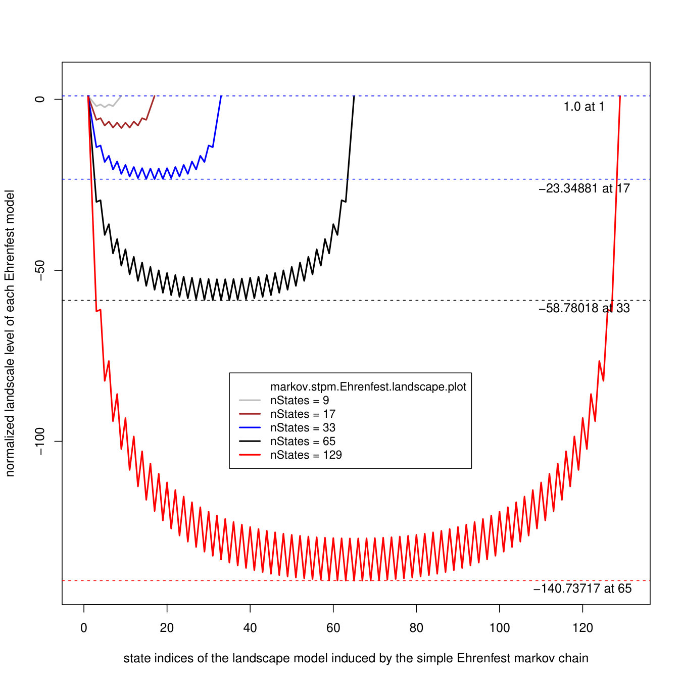 Figure 1
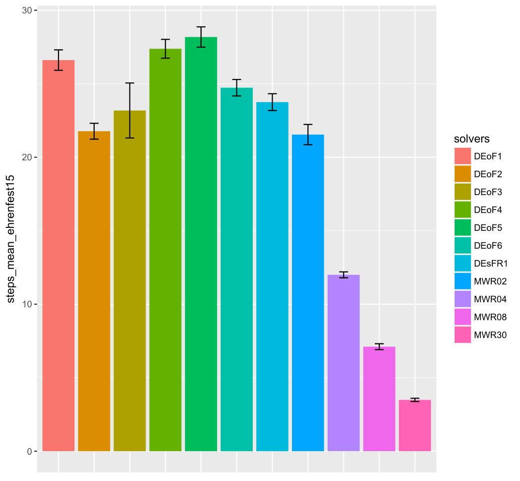 Figure 2
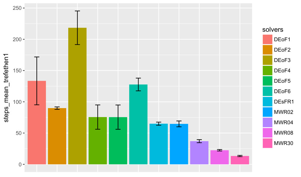 Figure 3
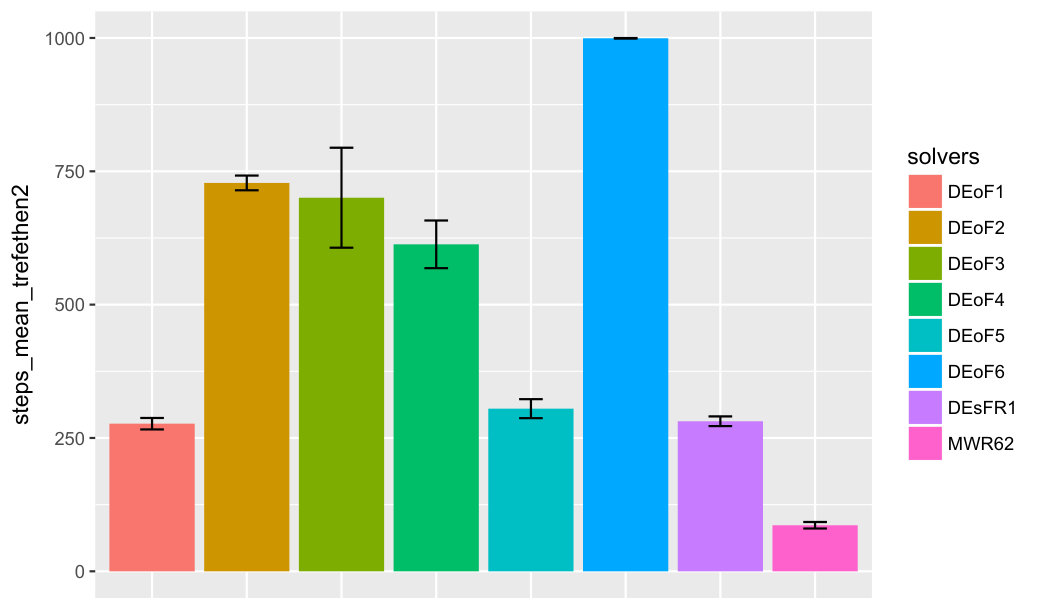 Figure 4
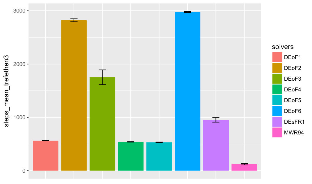 Figure 5
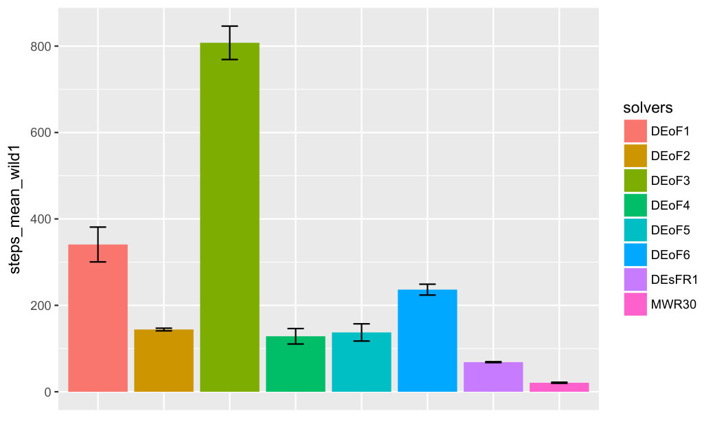 Figure 6
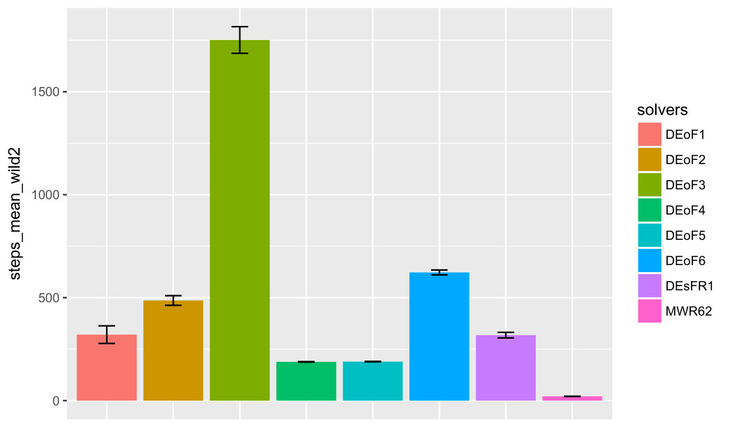 Figure 7
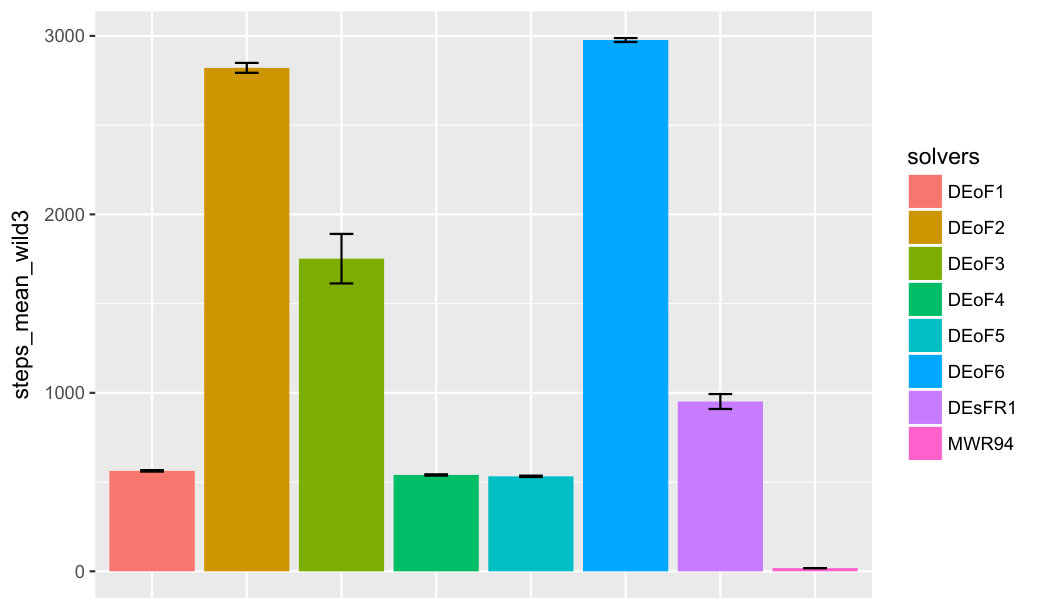 Figure 8
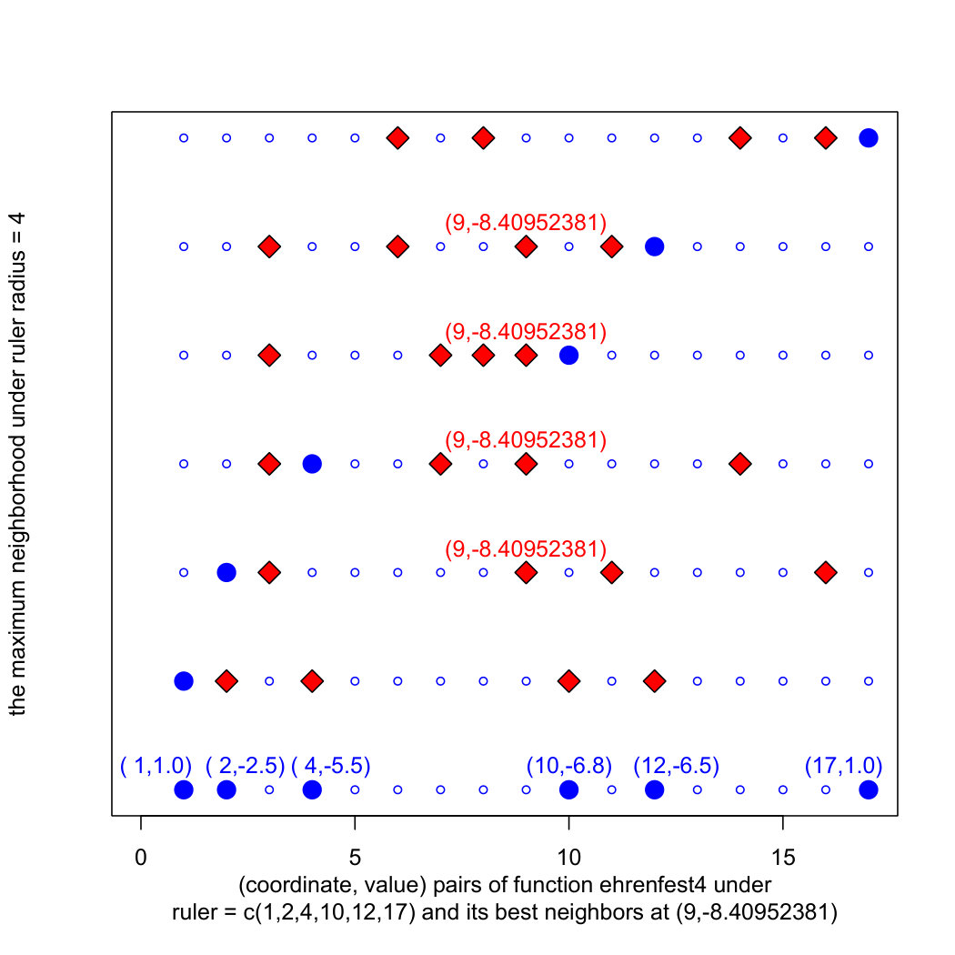 Figure 9
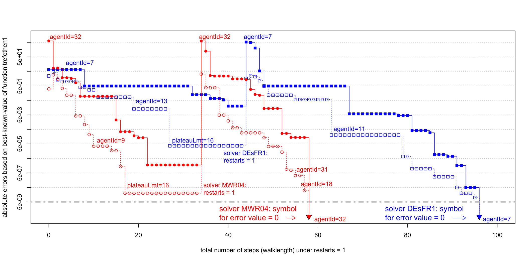 Figure 10
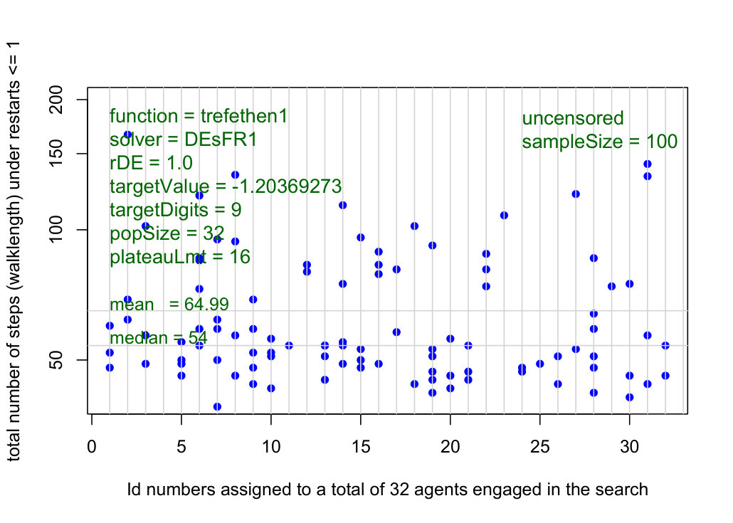 Figure 11
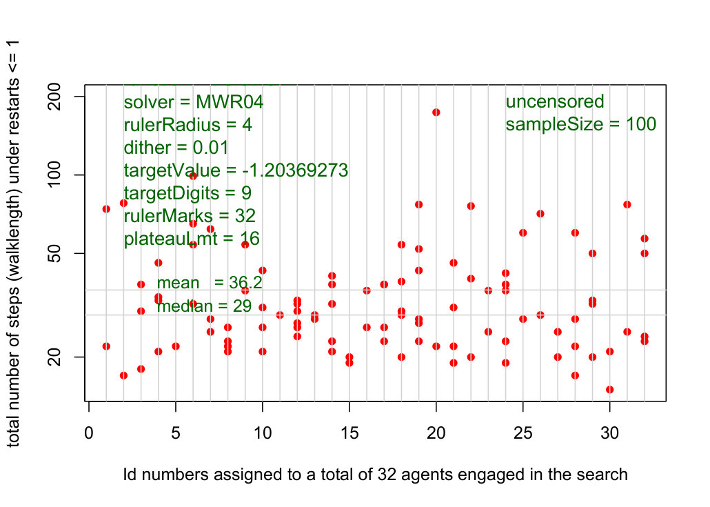 Figure 12
Peer Reviews
No public reviews on file for this paper yet. If you reviewed it on a platform where reviews are public (OpenReview, ICLR, NeurIPS, ICML), you can paste yours below so the community can read it here.
Videos
No videos yet. Explain this paper in a talk, walkthrough, or lecture? Add one.
Taxonomy
TopicsMatrix Theory and Algorithms · Quantum Computing Algorithms and Architecture · Neural Networks and Reservoir Computing
**On Uncensored Mean First-Passage-Time Performance Experiments
with Multiwalk in : a New Stochastic Optimization Algorithm **
**Summary. ** A rigorous empirical comparison of two stochastic solvers is important when one of the solvers is a prototype of a new algorithm such as multiwalk (MWA). When searching for global minima in , the key data structures of MWA include: rulers with each ruler assigned marks and a set of neighborhood matrices of size up to , where each entry represents absolute values of pairwise differences between marks. Before taking the next step, a controller links the tableau of neighborhood matrices and computes new and improved positions for each of the marks. The number of columns in each neighborhood matrix is denoted as the neighborhood radius . Any variant of the DEA (differential evolution algorithm) has an effective population neighborhood of radius not larger than 1. Uncensored first-passage-time performance experiments that vary the neighborhood radius of a MW-solver can thus be readily compared to existing variants of DE-solvers.
This paper considers seven test cases of increasing complexity and demonstrates, under uncensored first-passage-time performance experiments: (1) significant variability in convergence rate for seven DE-based solver configurations, and (2) consistent, monotonic, and significantly faster rate of convergence for the MW-solver prototype as we increase the neighborhood radius from 4 to its maximum value.
[TABLE]
**On Uncensored Mean First-Passage-Time Performance Experiments
with Multiwalk in : a New Stochastic Optimization Algorithm **
Franc Brglez
Computer Science, NC State University
Raleigh, NC 27695, USA
**Abstract. ** A rigorous empirical comparison of two stochastic solvers is important when one of the solvers is a prototype of a new algorithm such as multiwalk (MWA). When searching for global minima in , the key data structures of MWA include: rulers with each ruler assigned marks and a set of neighborhood matrices of size up to , where each entry represents absolute values of pairwise differences between marks. Before taking the next step, a controller links the tableau of neighborhood matrices and computes new and improved positions for each of the marks. The number of columns in each neighborhood matrix is denoted as the neighborhood radius . Any variant of the DEA (differential evolution algorithm) has an effective population neighborhood of radius not larger than 1. Uncensored first-passage-time performance experiments that vary the neighborhood radius of a MW-solver can thus be readily compared to existing variants of DE-solvers.
This paper considers seven test cases of increasing complexity and demonstrates, under uncensored first-passage-time performance experiments: (1) significant variability in convergence rate for seven DE-based solver configurations, and (2) consistent, monotonic, and significantly faster rate of convergence for the MW-solver prototype as we increase the neighborhood radius from 4 to its maximum value.
I. Introduction
A rigorous empirical performance comparison of two stochastic solvers is of particular importance when one of the solvers is new and under investigation for potential improvements. The book on First-Passage Processes [1] explains that
… first passage underlies many stochastic processes in which the event, such as a dinner date, a chemical reaction, the firing of a neutron, or the triggering of a stock option relies on a variable reaching a specified value for the first time …
In the context of two stochastic solvers, the variable we monitor for reaching a specified value is the target value of the objective function. Typically, the target value is also the best-known-value (bkv) since the optimum value may not been proven. If the target value is not an integer, its value is specified by the total number of digits it contains before and after the decimal point. We define the first-passage-time (fpt) stopping criterion for any solver as the stopping time of the solver when it returns the target value for the first time. We say that a solver run is censored if it stops due to a timeout limit before reaching the target value. In this paper, we compare the performance of two stochastic solvers by repeating the experiment with at least 100 random seeds and evaluate the answer to this question: “what is the uncensored mean time for each solver to reach the same target value?” We say that the comparison is reliable if at least one of the solvers has 0 censored runs.
In contrast, typical computational experiments to rank the performance stochastic optimization solvers are based on a much simpler approach: take solvers, problem instances, random seeds, run each solver under the stopping criterion of a fixed runtime limit. Then, for each solver, tabulate distances from best-known-values and related statistics. In [2], most insights are revealed in Figure 2 which tallies successes with 18 solvers over all 100 runs for each of 48 objective functions. Here is a verbatim quote: “A ‘success’ was defined as a solution less than 0.005 more than the minimum of the objective function between the default bounds.” In other words, bkv a solution value bkv + 0.005. Our experiments with this stopping criterion show that solver rankings become increasingly unreliable as the percentage of censored results increases. This observation is also supported with arguments by statisticians [3]. Under criteria defined in Figure 2, the percentage of censored results ranges from (4800 - 3800)/4800 = 21% to (4800 - 1200)/4800 = 75%. If the error tolerance that defines a ‘success’ is reduced from 0.005 to 0.0005, the percentage of censored results in Figure 2 is most likely to increase rapidly towards 100%.
In this paper, the concept of first-passage-time and runtime limit is measured in units that are platform-independent: on a granular scale we count the number of objective function evaluations (probes). On a higher level, we report the rate of solver convergence towards the target value by counting the number of iterations or steps. We replace the value of runtime limit with the value of iterations/steps limit.
II. Background and Motivation
In a seminal paper Kac explains the Ehrenfest model of diffusion with an state-transition probability matrix and makes a connection to random walks on graphs [4]. As part of an on-going research to be reported elsewhere, we have transformed this matrix to an objective function ehrenfest(x) defined on the set of integers in the range . See Figure 1 for plot of function values for . The adjacent bargraph represents a template that summarizes a statistical experiment with sampleSize = 100, reporting the mean values of steps returned by each of 11 solver configurations upon finding the minimum value solution for the function ehrenfest15(x). All parameters relevant to results in this bargraph are summarized in the table below:
OFname = ehrenfest15 solvers are configured for nStates = 2^15 + 1 first-passage-time stopping coordBest = 16384, 16386 DEoF1, DEoptim, strategy=1 valueTarget = -78544.9529 DEoF2, DEoptim, strategy=2digitsTarget = 9 DEoF3, DEoptim, strategy=3 OFtol = 5e-04 DEoF4, DEoptim, strategy=4 rulerMarks = 32 DEoF5, DEoptim, strategy=5 agentId = 1,2,..,32 DEoF6, DEoptim, strategy=6 dither = 0.01 DEsFR1, simpleDE, restarts, r=1neighbRadius = 2,4,8,30 MWRxx, multiwalk, xx=2,4,8,30 We briefly explain the solvers and the most important names and values of variables in this table. The first six solvers, DEoF1 to DEoF6 represent six configurations of the same solver DEoptim, readily accessible as an R-package [5]. A very useful property of DEoptim is that it accepts a user-defined entry for valueTarget, which then allows for implementation of the first-passage-time stopping criterion. Importantly, we must pass the variable targetDigits to the objective function so that the value returned by the objective function is ’quantized’ with the R-command ’signif’. For example, signif(1234.5789 - 0.0004999, 9) returns 1234.5784 in R-shell.
The solver DEsFR1 is our extension of ’simpleDE’ code supplied with the R-package ’adagio’ [6]. The code has been extended to support both the first-passage termination criterion as well as restarts, matching the capabilities of solver HWR. The most important data structures in HWR are the ruler, the maximum ruler neighborhood, and the neighborhood radius. The number of marks in the ruler is equivalent to the size of population in DE-based solvers. For details, see Section III.
By default, valueTarget, digitsTarget represent the best-known-value of the objective function, expressed with 9 digits. In the spirit of [8], we maintain digitsTarget = 9 for each valueTarget associated with each objective function and with each solver.
The consistent performance of the four multiwalk solver configurations HWRxx is a great motivator to review its details in the next section. As we increase the neighborhood radius from 2 to the maximum of 30, the mean number of steps reduces from 21.5 to 3.5!
For DE-based solvers, the best best mean value of 21.77 steps is returned by solver DEoF2 under the strategy=2 configuration. The increase in standard error observed for solver DEoF3 is due to a single run that has been censored at 200 steps. The next best mean value of 23.75 steps is returned by solver DEsF1, our extension of ’simpleDE’ code supplied with the R-package ’adagio’ [6]. The bargraph in Figure 1 is a template for the harder test functions introduced in Figure 5.
III. The Multi-Walk Algorithm (MWA)
To outline the intuition that underlies the multi-walk algorithm without loss of generality, we use a simple example of search for the minimum of the function ehrenfest(x) in Figure 1. The function ehrenfest4(x) is defined on the range : we select randomly 4 points in this range, say 4,12,10,2. The choice of integers is for simplicity only. By combining the two end points from the range and the four random points into an ordered arrangement of marks, we construct the ruler:
[TABLE]
Next, we consider a complete graph with vertices and edges, where marks serve as coordinates for each vertex. We define weight of each edge as the absolute value of differences between each pair of marks. The resulting structure is called the ruler difference matrix, shown in Figure 2. Creating this matrix is only an intermediate step, what we need is the ruler neighborhood matrix next to it: it has rows and columns. The number of columns in each neighborhood matrix is denoted as neighborhood radius . The red marks in the adjacent plot represent coordinate positions of difference in the ruler neighborhood matrix. Moreover, the ruler coordinates at the bottom of this plot are presented as (coordinate,value) pairs where each value is computed by evaluating the function ehrenfest4(x). Since, for this function, valueTarget=-8.40952381, the pair (9,-8.40952381) is the solution found by this search already on step=1.
For steps , the multi-walk can be formulated recursively:
[TABLE]
….. the matrix of ruler coordinates
….. the matrix of objective function values
…. the ruler neighborhood matrix
….. the R-based implementation in Figure 3
The implementation of MWA in Figure 3 has two main parts: the left column implements MW without the support for random restart, the column on the right implements MWR which supports a random restart. At the bottom of the column on the right, we show a snippet of the original code from [6]. A statement agentId = which.min(F) is contained in both MW and MWR. This statement accesses the value of not only valueBest of the objective function but also agentId as a number from the range ; a number reported as the index of the mark that reaches valueTarget. See Figure 4.
There are traces of four walks in Figure 4. The MW-solver engaged a ruler with 32 marks and a radius of 4, i.e. only 4 neighbors (from the maximum of 30) are considered as candidates for the next step. Since agentId=32 is the first to reach the target value on step=59, the walk with solid line reports its position for the full duration of the walk. We have a similar arrangement for DE-solver where agentId=7 is the first to reach the same target value, but now on step=95.
Results in Figures 2 and 4 support our intuition that underlies the multiwalk algorithm. By associating the ruler-based coordinates with differences of such coordinates creates the global neighborhood as the key to accelerating the convergence of MWA. The most significant observation we make about the experimental results in Figure 4 is this: a neighborhood with a radius of only 4 (from a maximum of 30) reduces the number of steps from the mean value of 64.99 for the DE-solver to 36.2 for the MW-solver. The best choices of parameters such as dither that adds a controlled amount of noise to each entry in the neighborhood matrix (default is at 1% or less), and the *tableauLmt *(default is the number of marks in each ruler) to control restarts, will be discussed elsewhere.
IV. Experiments and Compararisons
For a summary of first-passage-time experiments with eight solvers and two groups of three hard-to-solve functions, see Figure 5. The number of rulers associated with each function increases from 1 to 3. Function wild1 is from [5], functions trefethen2, trefethen3 are from [8].
V. Summary and Future Work
We expect to observe consistent and improved rate of convergence with MW-solvers also for other hard test instances in continuous domain. As we increase the neighborhood radius, the increasing cost of computing the neighborhood matrix can be balanced with a parallel implementation.
An adaptation of multiwalk concepts to hard problems in discrete domains will likely accelerate the convergence rate in comparison with the current state-of-the-art stochastic solvers such as reported in [9], [10], and [11].
Acknowledgements. The solver DEoptim [5] provided a robust foundation which we could not do without. The elegance of simpleDE under [6] is a model for our implementation. Suggestions from Dr. Larry Nevin are much appreciated.
The reference list from the paper itself. Each links out to its DOI / PubMed record.
- 1[1] Sidney Redner. A Guide to First-Passage Processes . Cambridge University Press, 2001.
- 2[2] Katharine Mullen. Continuous Global Optimization in R. Journal of Statistical Software, Articles , 60(6):1–45, 2014.
- 3[3] Pranab Kumar Sen. Censoring in Theory and Practice: Statistical Perspectives and Controversies. Institute of Mathematical Statistics, Analysis of Censored Data , 27:177–192, 1995.
- 4[4] Mark Kac. Random walk and the theory of Brownian motion. The American Mathematical Monthly , 54(7P 1):369–391, 1947.
- 5[5] Mullen, K.M, Ardia, D., Gil, D., Windover, D., Cline, J. D Eoptim: An R Package for Global Optimization by Differential Evolution. Journal of Statistical Software . URL http://www.jstatsoft.org/v 40/i 06/ , 40(6)(1–26), 2011.
- 6[6] Hans Werner Borchers. Package ‘adagio’: Discrete and Global Optimization Routines. https://cran.r-project.org/package=adagio, 2018.
- 7[7] Wikipedia. Golomb Ruler. Published under http://en.wikipedia.org/wiki/Golomb_ruler , 2018.
- 8[8] Folkmar Bornemann, Dirk Laurie, Stan Wagon, and Jorg Waldvogel. The SIAM 100-digit challenge: a study in high-accuracy numerical computing , volume 86. SIAM, 2004.