Improvement of optical image by measurement reduction technique at parametric multiplexing
D. A. Balakin (1), A. S. Chirkin (1, 2) ((1) M. V. Lomonosov Moscow, State University, Faculty of Physics, (2) M. V. Lomonosov Moscow State, University, The International Laser Center)

TL;DR
This paper demonstrates how measurement reduction techniques can enhance the quality of optical images obtained through parametric multiplexing, leveraging quantum correlations and prior object information.
Contribution
It introduces a novel approach combining measurement reduction with parametric multiplexing to improve optical image quality using quantum correlations and object sparsity.
Findings
Enhanced image quality through measurement reduction.
Utilization of quantum correlations in multiplexed images.
Improved image reconstruction by incorporating object sparsity.
Abstract
In the process of parametric optical image amplification, images are formed at new frequencies in addition to the amplified original image. We show that the parametric multiplexing of optical images can be used to produce an image with improved quality. As an example, we study the parametric amplification of an optical image at low-frequency pumping in which multiplexed optical images turn out to be quantum-correlated. Additional improvement is made possible by using the information about the object that is available to the researcher, in particular, about sparsity of its image. To take the available information into account, we apply the measurement reduction technique.
Click any figure to enlarge with its caption.
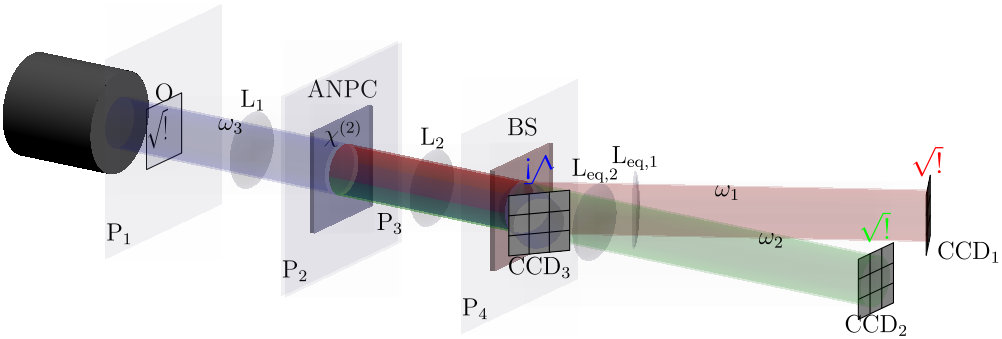 Figure 1
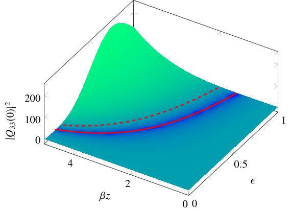 Figure 2
 Figure 3
 Figure 4
 Figure 5
Peer Reviews
No public reviews on file for this paper yet. If you reviewed it on a platform where reviews are public (OpenReview, ICLR, NeurIPS, ICML), you can paste yours below so the community can read it here.
Videos
No videos yet. Explain this paper in a talk, walkthrough, or lecture? Add one.
Improvement of optical image by measurement reduction technique at parametric multiplexing
D. A. Balakin
M. V. Lomonosov Moscow State University, Faculty of Physics, Leninskie Gory, 1, bld 2, Moscow 119991, Russia
A. S. Chirkin
M. V. Lomonosov Moscow State University, Faculty of Physics, Leninskie Gory, 1, bld 2, Moscow 119991, Russia
M. V. Lomonosov Moscow State University, The International Laser Center, Leninskie Gory, 1, bld 62, Moscow 119991, Russia
Abstract
In the process of parametric optical image amplification, images are formed at new frequencies in addition to the amplified original image. We show that the parametric multiplexing of optical images can be used to produce an image with improved quality. As an example, we study the parametric amplification of an optical image at low-frequency pumping in which multiplexed optical images turn out to be quantum-correlated. Additional improvement is made possible by using the information about the object that is available to the researcher, in particular, about sparsity of its image. To take the available information into account, we apply the measurement reduction technique.
Introduction
As it is well-known, in traditional parametric amplification of an optical image with high-frequency pumping, an additional image appears at the so-called idle frequency (see, for example [1, 2]). In the case of processes of optical parametric amplification with low-frequency pumping that can be realized in coupled parametric processes [3, 4, 5] optical images are formed at more than two frequencies [6, 7, 8, 9, 10]. In other words, in coupled parametric interactions frequency multiplexing of optical images occurs. The quantum theory of such interactions is developed in [6, 7, 8, 10], where various parametric image amplification schemes are examined. Experimental studies on the optical image multiplexing are presented in the articles [9, 10].
In the works [6, 7, 8] optical image quality is characterized by the signal-to-noise ratio (SNR). It is established that SNR of the image at the main frequency decreases in spite of increasing the mean photon number. Meanwhile, SNR of the images at additional frequencies increases along with their mean photon number.
Recently, image multiplexing has been used in ghost image acquisition schemes [11, 12, 13, 14, 15, 16, 17]
It is shown in our works [11, 12, 13, 14] that using quantum correlations of ghost images and the reduction technique in image processing, we can improve the characteristics of the reconstructed optical image.
The purpose of this paper is to study the quantum correlations of optical images during their multiplexing in two coupled parametric processes and apply the method of measurement reduction for obtaining an optical image with improved quality. The analysis is based on the coupled parametric interactions that realize parametric image amplification with low-frequency pumping, and the scheme with far-away object is considered. Note that some issues of such a process are studied in [7].
This process is of particular interest when the wavelength of the original image is in the ultraviolet range and the pump radiation wavelength of the conventional three-frequency interaction falls within the absorption region of a nonlinear crystal. The process of parametric amplification with low-frequency pumping allows the use of visible radiation as pumping, while the images at additional frequencies will be in the near-infrared range.
The article structure is as follows. In section 1, we discuss the optical setup for image amplification and multiplexing and the parametric processes taking place therein. In section 2 a specific variant of the optical setup is considered and the photon number means, variances and covariances are derived. In section 3 the measurement model and the measurement reduction method is outlined, including the notions of a measuring transducer, an ideal measuring transducer and the conditions for the possibility of image reconstruction. The information about the object that is available to the researcher and that is employed in reduction is summarized in subsection 3.1. In subsection 3.2, the algorithm of image processing using reduction method that takes this information into account is described. Computer modeling results are given in section 4. Main results of the article are summarized in the conclusion.
1 Amplification and multiplexing of an optical image
The scheme of parametric optical image amplification is depicted in Fig. 1. The weak optical image that is to be amplified is located in the object plane . This image is projected by the lens onto the input of an aperidic nonlinear photon crystal (ANPC), for example, LiNbO3, in which coupled parametric interactions, specifically, down- and up-conversion processes, occur simultaneously. The amplified image and the images generated at two new frequencies (see below) are projected by the lens from the output of the crystal (plane ) onto the image plane . The lenses and have the same focal length . The object and image planes, as well as the input and the output of the ANPC, are at the distance . This is the scheme with the so-called far-away object, it is similar to the scheme considered in [2, 7].
We denote the field operators in the object and the image planes as and , respectively, and those in the input and the output planes of the NPC as and , respectively. The index is associated with the wavelength . The operators , and , are related by the Fourier transformation performed by the lens
[TABLE]
and by the lens
[TABLE]
is the pupil frame function that accounts for the finite area of the pupil. Taking it into account is necessary for the correct analysis of the image amplification scheme [2] due to vacuum fluctuations outside of the pupil’s aperture, described by the operator (the second term in Eq. (2)). However, they do not contribute to any normal-ordered operational expressions associated with measurable values, so we omit this term below. Therefore, the expression (2) can be presented as
[TABLE]
where and are the Fourier transforms of and , respectively:
[TABLE]
is the transversal wave vector.
All operators under consideration , , and obey the commutation relations
[TABLE]
where is the direction of wave propagation. Mean value of the operator is the mean photon flux density in cross-section , measured in photons per cm2.
To find the connection between operators and , i. e. the connection between fields at the output and the input of the ANPC, it is necessary to consider the nonlinear processes in the ANPC. The processes under study are two coupled processes
[TABLE]
Here is the frequency of intense pump wave, and , and are the frequencies of generated waves with and being the shared frequencies of two processes. The first down-conversion process in Eq. (6) represents parametric amplification during high-frequency pumping, and the second one is the up-conversion process. They can be implemented simultaneously in an aperiodical NPC.
In the undepleted pump plane wave approximation taking into account the diffraction phenomenon the processes in Eq. (6) can be described by the system of equations
[TABLE]
Here is the transversal Laplacian, and are the creation and annihilation operators of photons with frequency () respectively, and are real nonlinear coupling coefficients that are proportional to second order nonlinear susceptibility and the absolute value of pump wave amplitude [3]. Eqs. (7) are derived for a lossless ANPC and for interaction of monochromatic waves.
The system of Eqs. (7) is solved by applying Fourier transform
[TABLE]
after which the Eqs. (7) become
[TABLE]
where , .
In the matrix form the solution of Eqs. (9) has the form
[TABLE]
where is determined by the values of the operators at ANPC input (), the index denotes transposition. In the case considered below, the operators , describe the vacuum state and the operator describes a coherent state.
The matrix consists of transfer functions :
[TABLE]
The functions are the self-transfer functions because they describe the amplification at frequencies (), while the cross-transfer functions describe the conversion from frequency to . Elements of the matrix (11) can be found in [7] and are not given here due to being cumbersome.
2 Formulation of the problem
In the previous section, the quantum theory of two coupled parametric processes is presented in relation to amplification and frequency conversion of an optical image, which can arrive at the nonlinear crystal at any of the frequencies , or . Here we turn to the case when the image with a mean photon number density is fed to the crystal in a coherent state at the frequency . In the framework of the monochromatic waves under consideration, results given below are valid if the image registration time is less than the characteristic time of image change, for example, the correlation time.
In the image plane , the mean photon number over pixel area in the amplified image and the additional ones is given by the expressions
[TABLE]
As expected, the output optical images are inverted relative to the initial image. It is important to note that the scales of output images at different frequencies are different, and the change in spatial scale is determined by the coefficient , where is the image wavelength. It should be noted that this fact was not taken into account in [7].
Different image scales somewhat complicate the reduction algorithm, as this means that sizes of pixels are different in different arms. One can proceed further in several ways.
- •
In the general approach without the assumption that the image is piecewise constant (see sec. 3), dealing with different pixel sizes in different arms is avoided, since in the infinite-dimensional case pixel size does not affect image representation.
- •
The images can be rescaled during processing if sensor point spread functions allow to do this both accurately and without loss of data.
- •
Finally, one can bring the images to the same scale using additional lenses. This approach is considered below.
It should be noted that these approaches provided the same results when they are valid.
In the image plane , images with different frequencies are directionally separated (for example, using a prism). A lens with the focal distance () is placed on the path of radiation with frequency in order to bring the image to the spatial scale that coincides with the scale of the image at the frequency . The lens is located at a distance from the plane and a distance to the measurement plane. The specified distance must satisfy the lens formula
[TABLE]
In this case, the distribution of the image mean photon number in the optically conjugate plane is given by ():
[TABLE]
According to Eq. (14), to match the image scales at the wavelengths and the ratio
[TABLE]
must be satisfied. Under this condition, we have
[TABLE]
The photon number variances are given by the following formulas
[TABLE]
Finally, the mutual correlations of the image fluctuations (covariances) between different frequencies
[TABLE]
have the forms
[TABLE]
[TABLE]
[TABLE]
To estimate the above moments, we use their values at . In this case, the matrix elements (11) have a simple analytical form:
[TABLE]
where . as a function of and is shown in Fig. 2.
It follows from Eq. (22) that the amplification of image takes place if .
In the absence of a down-conversion process () and, therefore, without generation of additional frequencies, there is no amplification. In the coupled parametric process under the condition , the original image initially decays and at the interaction length , , the mean photon number of the image becomes zero. The image gain process begins after the interaction length , (see also Fig. 2). As for the photon numbers , at frequencies and , they monotonously grow as the interaction length increases according to expressions (12), (22).
3 Processing of acquired images
The output of sensors in the -th arm, denoted as , can be considered as the output of a measuring transducer (MT) for input signal .
We will consider piecewise constant images, i. e. transparency of the research object is constant within each pixel. Areas of constant transparency and constant brightness corresponding to pixels are considered to be ordered in an arbitrary but fixed way. Due to that it is sufficient for us to consider a finite number of values of . Thus, as the vector of transparencies is an element of finite-dimensional Euclidean space .
This assumption is made for simplicity (in order to avoid working with infinite-dimensional spaces) and is not crucial to the reduction method. For examples of reduction in the infinite-dimensional case see, e. g., [18, ch. 10] and [19]. If the assumption is invalid, the estimate of the algorithm below estimates linear combinations of around the values of determined by locations of the sensors with weights that are dependent on the MT and the ideal MT specified by the researcher (see below). For example, if sensors have uniform light sensivity throughout their area, the ideal MT corresponds to unit-sized sensors of unit size and the images were acquired by sensors that are several times larger, is averaged over unit-sized areas centered at sensor locations.
Let us formulate the measurement model as
[TABLE]
where is an unknown vector that describes the transparency distribution of the object, is the measurement error with zero expectation, , which means absence of systematic measurement error, and covariance matrix . The dimension of vector is the number of pixels in the object image, while the dimension of is the total number of sensors. The condition of systematic measurement error absense means, in particular, that the expectation of the component of measurement results caused by sensor dark noises is subtracted from the measurement results, similar to [20, 14] for ghost images.
The matrix describes image amplification, multiplexing and acquisition: the matrix element is equal to the mean output of -th sensor for unit transparency of -th element of the illuminated object and zero transparency of other object elements (i. e. whose indices differ from ). Due to the measuring setup with three arms, it is a block matrix and consists of three blocks describing different arms:
[TABLE]
Under the conditions used to derive the mean numbers of photons, their variances and mutual correlations the matrices – are identity ones multiplied by the factor before in expression (16) for the mean numbers of photons. The matrices – model the sensors. Specifically, the matrix element is equal to the output of the sensor in -th arm at -th position for unit brightness of -th pixel of the image formed in that arm and zero brightness of other pixels. For the same reason, the noise covariance matrix has block form as well:
[TABLE]
Here the element with indices , of the block is equal to either photocount variance in Eq. (17) if or covariance of photocounts in Eq. (19)–(21) if for the same pixel ordering as in the matrix . Hence, the dependence of the matrix (25) on is caused by the dependence of variances and covariances on . The term is the covariance matrix of the noise component that is unrelated to parametric amplification and multiplexing, e. g. thermal noise in circuits, detection of outside photons, non-unit quantum efficiency of the sensors and their dark noise.
The objective of an image processing algorithm is to output the most accurate estimate of the signal from the measurement result , where the matrix describes a measuring device that is ideal (for the researcher). Hence, is the feature of the original image that is of interest to the researcher. We consider the case when the researcher is interested in reconstruction of the object image itself, and imaging does not distort the object, therefore, , where is the average number of photons per pixel of the illuminated object. One way of achieving this is the measurement reduction method described in [18], see also [21, 22, 23, 24]. If the estimation process is described by a linear operator ( is the result of processing the measurement ), the corresponding mean squared error (MSE) in the worst case of , , as shown in [18], is minimal for that is equal to the linear unbiased reduction operator
[TABLE]
where - denotes pseudoinverse. , and the covariance matrix of the linear reduction estimate is
[TABLE]
Estimation is possible (MSE is finite) if the condition holds, where, as noted above, characterizes the real measuring device, while characterizes an ideal one with the point spread function required by the researcher, and, therefore, the desired resolution, if this condition if fulfilled. This condition essentially means that only the features of the object that are measured by the real measuring device (that is, affect its output) can be estimated. Unlike fluorescence-based superresolution techniques, see e. g. [25], the proposed technique does not require attaching fluorescent molecules to the object. However, in addition to the above condition, the error of the obtained estimate can be too large to distinguish the signal from the noise in practice, and usually the better the desired resolution of the ideal measuring device compared to the resolution of the real one, the larger MSE of the obtained estimate. Nevertheless, by choosing one can select an acceptable (to him) compromise between obtained resolution and noise magnitude, that is, to estimate with acceptable resolution and with an tolerable noise level.
In the case under consideration, as seen from Eq. (24), the diagonal elements of – are nonzero. Therefore, each block of is non-degenerate, so for non-degenerate the reduction error takes only finite values.
The measurement reduction technique for the case when it is known that , where is convex and closed, in other words, when the feature of interest of the object is known to satisfy certain given constraints, was considered in [24, 26]. The linear estimate (26) is refined using this information by solving the equation
[TABLE]
for , where is the measurement reduction operator for a MT and noise with covariance matrix , and the operator
[TABLE]
describes orthogonal projection onto by minimizing the Mahalanobis distance associated with the covariance matrix (27) of the linear reduction estimate . The earlier version of reduction technique proposed in [13] and in [24] for similar information used minimization of the ‘‘ordinary’’ Euclidean distance instead of Mahalanobis distance. In [26], the advantages of minimizing Mahalanobis distance instead of Euclidean distance during projection are shown. For such prior information, the covariance matrix (27) of linear reduction estimate error is an upper bound on the covariance matrix of the obtained estimate .
3.1 Prior object information
It is obvious that a priori the transparency distribution of the object takes values in , hence , , where the average number of photons per pixel of the illuminated object is assumed to be known.
It is assumed that the transparency distribution of the object is not ‘‘entirely’’ arbitrary: transparencies of neighboring pixels usually do not differ much. As a result, the image is sparse (many of its components are zero) in a given basis, similarly to compressed sensing [27, 28, 29, 30]. The hypothesis ‘‘-th component in the given basis of the estimate is zero’’ is treated as a statistical hypothesis that is tested using the measurement data against the alternative that it is nonzero. Its testing is controlled by choosing the significance level (the probability of rejecting the hypothesis when it is true) of the rejection criterion or a parameter of the criterion that monotonously depends on it.
The researcher also knows the matrix (24) that describes image acquisition conditions and, up to the vector , the matrix (25) that describes the magnitudes of measurement errors. Note that the worst case of is realized if all pixels are equally transparent.
3.2 Reduction algorithm
The proposed algorithm of multiplexed GI processing using measurement reduction technique that is based on the indicated prior information has the following form.
Calculation of linear reduction estimate (26) based on the acquired images. For calculation of the covariance matrix (25), the worst case, that all pixels have the same brightness, is assumed. 2. 2.
Refinement of the estimate using the information by the method (28) by fixed-point iteration, i. e. by consecutive application of the mapping (28) with as the initial approximation. We denote the obtained estimate by . 3. 3.
Application of the sparsity-inducing transformation to . ‘‘Sparsity-inducing’’ means that the researcher expects the chosen transform of the true transparency distribution of the object to be sparse. 4. 4.
Calculation of the worst-case (in ) variances of the components of (the diagonal matrix elements of ) and calculation of in the following way: if , otherwise . 5. 5.
Inverse transformation of (if is a unitary transformation, then ), i. e. calculation of . 6. 6.
Calculation of the projection that is considered to be the result of processing.
The algorithm parameter reflects a compromise between noise suppression (the larger the value of , the greater the noise suppression) and distortion of images whose components are close to [math]. As mentioned above, the step 4 can be considered as testing statistical hypotheses (for the alternative ) for all . In this paper the criterion used in step 4 is based on Chebyshev’s inequality: if , then (hence, the significance level is at least ). Step 4 can be also interpreted as replacement of the original matrix with one whose kernel contains the estimate components after the specified transform that are affected by noise of the specified magnitude or more.
4 Computer modeling results
The results of image processing according to the described algorithm are shown in Figs. 3–7. The computer modeling was carried out for wave lengths 1.2\text{,}{\mathrm{\SIUnitSymbolMicro m}}^{-1}, $(\lambda_{2})^{-1}=$0.8\text{\,}{\mathrm{\SIUnitSymbolMicro m}}^{-1}, 3.2\text{,}{\mathrm{\SIUnitSymbolMicro m}}^{-1}, aperture area $S_{a}=$25\text{\,}{\mathrm{cm}}^{2}, pixel area 100\text{,}{\mathrm{\SIUnitSymbolMicro m}}^{2}, focal distance $f=$10\text{\,}\mathrm{cm} and the value of crystal parameter and the dimensionless crystal length indicated in figure captions, with ranging from to and ranging from to . The sensors in arms are identical ones that are three times as large as an element of the object image. Therefore, image processing via measurement reduction increases resolution in addition to noise suppression. It should be noted, however, that the objectives of superresolution and reconstruction of the image with a small number of photons are generally at odds with each other: relaxing resolution requirements allows to reconstruct the image using less photons, as less components of the image have to be recovered.
One can see that additional information about sparsity enables higher noise suppression without compromising reducing obtained resolution too much. Increase of leads to better noise suppression (cf., e. g., Figs. 3g and 3h), but also worse distortions caused by discarding ‘‘significant’’ image components as well (cf., e. g., Figs. 4e and 4f). Too large values of cause degradation of image fidelity due to distortion outweighing improved noise suppression, as small-scale image details are suppressed as well. Therefore, one should choose the maximal value of that preserves the details of interest. To do that, one can model processing of a test image that contains the required details and choose the largest value of that preserves them, or visually compare the reduction results for different and select its final value by ternary search.
The transform whose result for the transparency distribution of the object is sparse that is usually employed in image processing by the means of compressed sensing is discrete cosine transform (DCT) [28, 29, 30]. In [31], several transforms (identity transform, discrete wavelet transform and DCT) were reviewed and the advantages of DCT were shown. However, in [14] it was shown that Haar transform may be preferable in the case of a transparency distribution that contains areas of weakly changing transparency with sharp borders if these areas are large compared to the resolution of the ideal MT and the location of the borders is important to the researcher, since those features align well with the vectors of the Haar transform basis. As the object images in Figs. 3–7 are of this type, the sparsity-inducing transform used in these figures is the Haar transform.
In all these figures results of processing of all images are compared to results of processing of a single image, namely, the one with the best signal-to-noise ratio. Since processing only a single image means that some of the obtained measurements are discarded, this results in worse estimate quality, even if the sum of acquired images is not noticeably different from the best image. For example, in Fig. 5 one can see that the same values of cause more distortion when processing a single image. In Fig. 5i only a single component, corresponging to uniform transparency, remains in the result of processing a single image, while the same value of produces an acceptable, although suboptimal, image shown in Fig. 5g. Furthermore, in the general case of additional noise multiplexing provides the means for further noise suppression if noise photons in different arms are detected independently.
As far as the parameters of the ANPC are concerned, larger crystal length leads to more amplification and more photons. The improvement of the number of photons is especially large when is increased from to . The results do not depend on the value of the parameter as much.
Conclusion
The problem of recovering images acquired in photon-sparse conditions can be solved by taking advantage of the additional information available to the researcher about the measurement process and about the object. Alternatively one can make the detection conditions worse (e. g. use sensors with less resolution) while preserving the same estimation quality. In this work, the additional information about the object is the information that the object transparency distribution is not arbitrary, namely, transparencies of close pixels tend to be close. This information is formalized as sparsity of the result of a given transform of the transparency distribution, similar to compressed sensing.
In compressed sensing, as a rule, the measurement error is modeled as an arbitrary vector with bounded norm. In the proposed method it is modeled as a random vector, and selection of the estimate components which are considered to be zero is based on the statistical properties of the estimate components, namely, their variances. The use of covariances of the estimate components in addition to their variances is a subject of further research. Another subject of further research are the opportunities provided by multiplexing for analysis of the measurement data, e. g., for verifying the reliability of both the measurement model [32, 33] and the results of reduction [34].
We consider that computer modeling based on the developed algorithm showed high efficiency of the developed reduction technique for parametric amplification of images and frequency conversion in the sense of improvement of both their quality and their noise immunity.
Finally, we emphasize once again that we are dealing with parametric interaction with low-frequency pumping. The carrier wavelength of the original image may be in the ultraviolet range, while the pump frequency may belong to the visible range. Further applications of the measurement reduction technique to processing of quantum images are being developed. This work was supported by Russian Foundation for Basic Research, grant 18-01-000598 A.
Acknowledgments
The authors acknowledge discussions with Prof. A. V. Belinsky.
The reference list from the paper itself. Each links out to its DOI / PubMed record.
- 1[1] M. I. Kolobov, editor. Quantum imaging . Springer, N.Y., 2007.
- 2[2] M. I. Kolobov. The spatial behavior of nonclassical light. Rev. Mod. Phys. , 71(5):1539–1589, 1999.
- 3[3] E. Yu. Morozov and A. S. Chirkin. Consecutive parametric interactions of light waves with aliquant frequencies. J. Opt. A: Pure Appl. Opt. , 5(3):233–238, 2003.
- 4[4] A. A. Novikov and A. S. Chirkin. Coupled multiwave interactions in aperiodically poled nonlinear optical crystals. J. Exp. Theor. Phys. , 106(3):415–425, 2008.
- 5[5] A. S. Chirkin and I. V. Shutov. Parametric amplification of light waves at low-frequency pumping in aperiodic nonlinear photonic crystals. Journal of Experimental and Theoretical Physics , 109(4):547–556, 2009.
- 6[6] A. S. Chirkin and E. V. Makeev. Simultaneous phase-sensitive parametric amplification and up-conversion of an optical image. J. Opt. B: Quantum Semiclassical Opt. , 7(12):S 500–S 506, 2005.
- 7[7] A. S. Chirkin and E. V. Makeev. Parametric image amplification at low-frequency pumping. J. Mod. Opt. , 53(5-6):821–834, 2006.
- 8[8] E. V. Makeev and A. S. Chirkin. Quantum fluctuations of parametrically amplified and up-converted optical images in consecutive wave interactions. Journal of Russian Laser Research , 27(5):466–474, 2006.