On the massless tree-level S-matrix in 2d sigma models
Ben Hoare, Nat Levine, Arkady A. Tseytlin

TL;DR
This paper investigates the properties of massless tree-level S-matrices in 2d sigma models, revealing that unlike massive cases, they do not exhibit integrability features such as factorization and particle production is observed even in integrable models.
Contribution
It demonstrates that massless tree-level S-matrices in 2d sigma models lack the integrability-linked factorization seen in massive cases and explores IR ambiguities and T-duality effects.
Findings
Massless S-matrices fail to factorize in integrable models.
Particle production occurs in several integrable 2d models.
IR ambiguities can cause anomalies in S-matrix equivalence.
Abstract
Motivated by the search for new integrable string models, we study the properties of massless tree-level S-matrices for 2d sigma models expanded near the trivial vacuum. We find that, in contrast to the standard massive case, there is no apparent link between massless S-matrices and integrability: in well-known integrable models the tree-level massless S-matrix fails to factorize and exhibits particle production. Such tree-level particle production is found in several classically integrable models: the principal chiral model, its classically equivalent "pseudo-dual" model, its non-abelian dual model and also the SO(N+1)/SO(N) coset model. The connection to integrability may, in principle, be restored if one expands near a non-trivial vacuum with massive excitations. We discuss IR ambiguities in 2d massless tree-level amplitudes and their resolution using either a small mass parameter or…
Click any figure to enlarge with its caption.
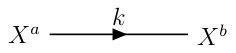 Figure 0
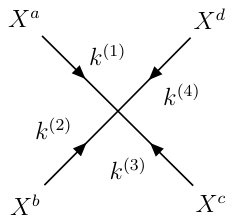 Figure 1
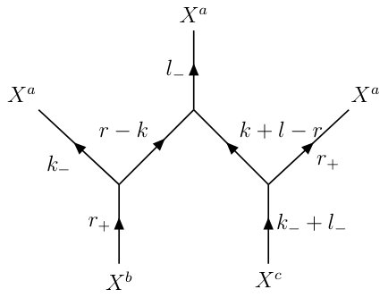 Figure 10
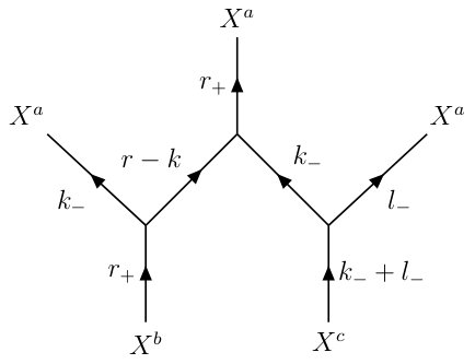 Figure 11
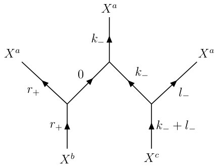 Figure 12
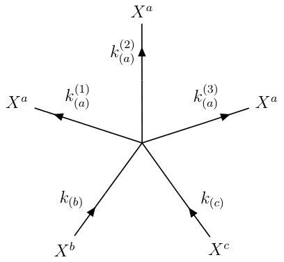 Figure 13
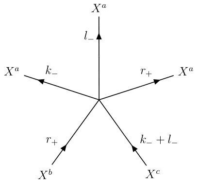 Figure 14
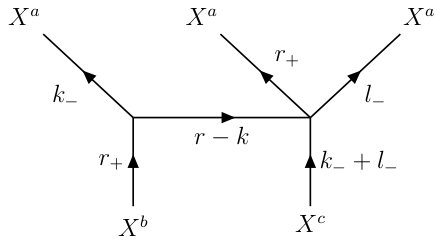 Figure 15
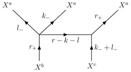 Figure 16
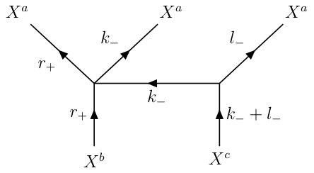 Figure 17
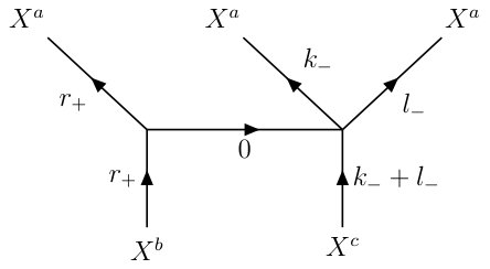 Figure 18
 Figure 19
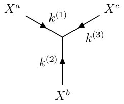 Figure 2
 Figure 20
 Figure 21
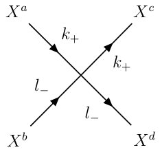 Figure 3
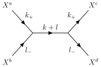 Figure 4
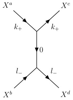 Figure 5
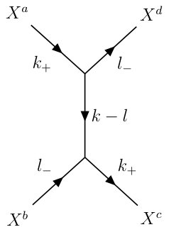 Figure 6
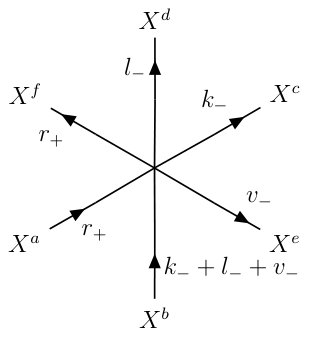 Figure 7
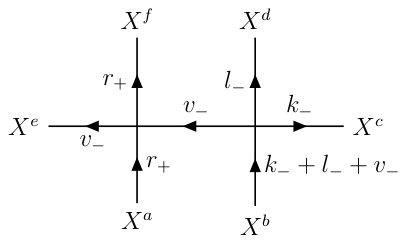 Figure 8
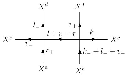 Figure 9
| PCM | PCMq | WZW | ZM | ZMq | NAD | -model | |
|---|---|---|---|---|---|---|---|
| p | 1 | 1 | 1 | 0 | 0 | 12 | |
| q | 0 | 1 |
| PCM | PCMq | WZW | ZM | ZMq | NAD | -model | |
|---|---|---|---|---|---|---|---|
| 1 | 0 | 3 |
| Colour factor | Colour-ordered amplitude | |
|---|---|---|
| 0 | ||
| 0 | ||
| 0 | ||
| 0 | ||
| 0 | ||
| 0 | ||
| 0 | ||
| 0 | ||
| 0 | ||
| 0 | ||
| 0 | ||
| 0 | ||
| Colour factor | Colour-ordered amplitude | |
|---|---|---|
| 0 | ||
| 0 | ||
| 0 | ||
| 0 | ||
Peer Reviews
No public reviews on file for this paper yet. If you reviewed it on a platform where reviews are public (OpenReview, ICLR, NeurIPS, ICML), you can paste yours below so the community can read it here.
Videos
No videos yet. Explain this paper in a talk, walkthrough, or lecture? Add one.
Imperial-TP-AT-2018-05
**On the massless tree-level S-matrix
in 2d sigma models**
Ben Hoare*a,[email protected], Nat Levineb,[email protected] and Arkady A. Tseytlinb,*333Also at Lebedev Institute and ITMP, Moscow State University. [email protected]
*a**ETH Institut für Theoretische Physik, ETH Zürich,
Wolfgang-Pauli-Strasse 27, 8093 Zürich, Switzerland.
bBlackett Laboratory, Imperial College, London SW7 2AZ, U.K. *
Abstract
Motivated by the search for new integrable string models, we study the properties of massless tree-level S-matrices for 2d -models expanded near the trivial vacuum. We find that, in contrast to the standard massive case, there is no apparent link between massless S-matrices and integrability: in well-known integrable models the tree-level massless S-matrix fails to factorize and exhibits particle production. Such tree-level particle production is found in several classically integrable models: the principal chiral model, its classically equivalent “pseudo-dual” model, its non-abelian dual model and also the coset model. The connection to integrability may, in principle, be restored if one expands near a non-trivial vacuum with massive excitations. We discuss IR ambiguities in 2d massless tree-level amplitudes and their resolution using either a small mass parameter or the -regularization. In general, these ambiguities can lead to anomalies in the equivalence of the S-matrix under field redefinitions, and may be linked to the observed particle production in integrable models. We also comment on the transformation of massless S-matrices under -model T-duality, comparing the standard and the “doubled” formulations (with T-duality covariance built into the latter).
Contents
-
2 Tree-level massless 4-point amplitudes in the principal chiral model and related -models
-
3 Higher-point amplitudes: particle production and non-factorization
-
A Comments on equivalence of massless S-matrix under field redefinitions
1 Introduction
Examples of integrable 2d models are few and hard to find. In the context of string theory, one is interested in finding new classically integrable 2d -models (see, e.g., [1] and refs. there). As a direct search for a Lax pair is generally complicated without additional clues such as symmetries, one may hope that the study of (classical) S-matrix may provide a useful guide. Indeed, a standard strategy in construction of massive integrable 2d theories is to require that the S-matrix satisfies the conditions of no particle production and factorization [2, 3, 4].111The existence of higher conserved charges implies (i) the absence of particle production and (ii) equality of sets of initial and final momenta. Combined with locality and causality this further implies (iii) factorization of amplitudes into products of ones. Expanded near a trivial flat vacuum, the -model describes an interacting theory of a set of massless 2d scalar fields. If integrability were equivalent to the factorization of their S-matrix, one could in principle use it to determine which couplings , , etc., i.e. which target space geometries, correspond to integrable models.
As we will demonstrate below, the connection between classical integrability and the factorization of the tree-level S-matrix breaks down in the case of massless 2d scalar scattering: well-known integrable models happen to have non-zero particle-production amplitudes. Thus the absence of tree-level massless particle production cannot be used as a criterion in search for integrable models.
To maintain the link to integrability one should instead consider the expansion near non-trivial vacua where excitations are massive.222More generally, one may try to consider the scattering of non-trivial massive solitonic states. To give a simple example, consider a massive 2d model with an integrable potential . This can be generalized to a -model by adding two “light-cone” directions as333For examples of such models see, e.g., [5] and refs. there. . Expanded near the trivial vacuum this -model will have non-zero S-matrix elements for any number of massless -excitations and a non-zero even number of -excitations, which may not, in general, factorize. At the same time, if we expand near the “light-cone” vacuum then the -excitations will be massive and their S-matrix will be factorizable for an integrable potential . This generalizes to other cases, with a familiar example being the expansion near the BMN geodesic in models (see, e.g., [6, 1]).444Given a -model model with target space that has at least one isometry , one can expand near classical solutions of the type with the remaining fields constant. This can give masses to some subset of the excitations; however, their interactions will typically break Lorentz invariance and hence the resulting massive S-matrix will not be Lorentz invariant. This is the case for the expansion near the BMN geodesic in models. Whether the factorization of such an S-matrix should be correlated with the integrability of the -model on in general is a priori unclear.
Returning to the perturbative expansion near a trivial “massless” vacuum, let us recall that for massless 2d theories the standard physical interpretation of the S-matrix may not apply since space is 1-dimensional and particles moving in the same direction do not separate asymptotically.555Still, massless S-matrices were formally discussed for integrable theories in the context of a finite-density TBA [7]. The S-matrix there retains the interpretation as the relative phase when one particle is moved past another. A related issue is the appearance of IR divergences at the quantum level [8]. Despite this, one is certainly able to formally define the massless S-matrix at the tree level, e.g., from the classical action evaluated on a solution with special scattering boundary conditions. Therefore, one may still ask if the resulting massless S-matrix should somehow reflect the classical (non-)integrability of the theory. This could be expected given that the standard definition of classical integrability via the existence of a Lax pair representation of the equations of motion makes no distinction between the massless and massive cases.
In some early work, this relation between classical integrability and the massless S-matrix was indirectly called into question. It was found in [9] that the S-matrix of the Zakharov-Mikhailov (ZM) model [10, 11] exhibits particle production: there are non-zero tree-level amplitudes with different numbers of incoming and outgoing particles. This appears to violate the usual intuition from integrability: the ZM model is classically integrable (admits a Lax pair) since it is classically equivalent to the principal chiral model (PCM).
Somewhat confusingly, it was taken for granted in [9] that particle production should be absent in the tree-level massless S-matrix of the PCM, while this was only known to be the case for the non-perturbative massive S-matrix [2]. Consequently, the presence of particle production in the ZM model was interpreted as implying an inequivalence of the PCM and ZM model at the level of the classical S-matrix.666The two models are, of course, quantum-inequivalent having opposite 1-loop -functions [9].
In fact, the standard argument that integrability implies the absence of particle production and factorization formally applies only to the massive case [4, 3].777In particular, the proof [4] that the existence of at least two higher conserved charges implies factorized scattering uses separation of wave packets which is not possible in the massless case. Indeed, it was later pointed out in a little-known work [12] (which was apparently independent of [9]) that the tree level massless S-matrix does exhibit particle production in classically integrable -models such as the -model and PCMq (the PCM with a WZ term with coefficient ).888The S-matrix trivialises [12] in the critical WZW case () when the left and right modes decouple. It was thus suggested [12] that, in contrast to what is well-known for massive theories [13], these massless scale-invariant 2d theories do not exhibit a direct relation between classical integrability and factorized tree-level scattering (or absence of particle production). In turn, demanding factorization of the tree-level S-matrix may not, in general, be necessary for the integrability of classical scale-invariant 2d models with massless excitations.
That this point remains little known and somewhat controversial is illustrated by the recent work [14]. There, considering a theory of Hermitian matrix-valued massless fields with 2-derivative interactions, an alternative definition of particle production was proposed based on the partial colour-ordered amplitudes, as opposed to the full amplitudes. Imposing the constraint of no tree-level particle production (in the sense of this alternative definition) was claimed to lead one directly to the action of the integrable PCM. However, it is unclear how to generalize this procedure to other integrable -models that do not have a notion of colour-ordered amplitudes (see Appendix C below).
Massless 2d S-matrices were also discussed recently in non-renormalizable (non scale-invariant) Nambu-like models [15, 16]. In this case there are no IR divergences (provided each scalar appears in the action only through its derivative)999Note that this is particular to a Nambu action for a string moving in flat space, but is not generally so in the case of a curved target space. and thus ambiguities related to IR poles appear to be absent, not only at the tree level but also at the loop level. Here the (naively expected) relation between factorization of the massless S-matrix and integrability does appear to hold (with the Nambu action being integrable beyond tree level only in special critical dimensions).101010The corresponding 2d massless S-matrix was suggested to be a useful tool in trying to understand the world-sheet theory for a confining QCD string [17].
Our aim is to clarify the properties of tree-level massless scattering amplitudes in bosonic 2d -models. Our basic examples will be the principal chiral model (PCM) and models related to it by dualities – the classically dual Zakharov-Mikhailov (ZM) model [10] and the non-abelian dual (NAD) model [18, 19]. We shall also consider the generalization PCMq that includes the WZ term, and the classically dual ZMq model, as well as the -model [20] that interpolates between the WZW model and the non-abelian dual of the PCM. These models are classically integrable, admitting a Lax pair, as will be reviewed in section 2.1. We will be interested in their tree-level S-matrices in the trivial vacuum where the basic excitations (taking values in the Lie algebra) are massless.
As will be discussed in section 2.2, scattering amplitudes of massless excitations in such scale-invariant 2d theories may have “0/0” ambiguities due to vertices and internal propagators vanishing simultaneously when the external momenta are taken on-shell. To resolve these ambiguities requires the use of a particular IR regularization prescription. The two standard ones that we shall use are the -regularization of the massless propagator and the massive regularization where all massless fields are given the same small mass, which is set to zero after momentum conservation is imposed and the amplitude is taken on-shell.
The simplest non-trivial 4-point amplitudes in the above models will be computed in section 2.3. We shall find that despite the classical equivalence of the PCMq and ZMq models their 4-point amplitudes are not the same – they differ by an overall coefficient. The same is true also for the PCM and its path integral dual – the NAD model.111111That the tree-level 4-point amplitude in the NAD model is different from the one in the PCM was first found in [21] and this disagreement was interpreted there as being due to IR ambiguities in computing massless scattering in 2 dimensions.
Various 5-point and 6-point amplitudes will be computed in section 3, demonstrating that, despite their classical integrability, the above models exhibit particle production and/or absence of factorization of their massless S-matrices. We shall first show that there are non-vanishing massless amplitudes in the PCM and the coset -model (confirming an earlier observation in [12]). The same conclusion will be reached for amplitudes: they are non-vanishing not only in the ZM model (as originally found in [9]), but also in the NAD model and the PCMq (with ).
Another context in which the massless 2d scalar S-matrix has been discussed is 2d scalar-scalar (or T-) duality [22]. One might a priori expect that S-matrices of two T-dual -models should be essentially equivalent (directly related up to a sign flip depending on the numbers of chiral scalars in the process). This property becomes manifest [22] in the “doubled” formulation of a -model [23] where the left and right chiral scalar modes are represented [24] by independent off-shell fields. As we shall discuss in section 4, the massless S-matrices computed in the standard and doubled approaches may, in general, differ in a non-trivial way, as they correspond to different choices of how to resolve the IR ambiguities. In particular, the S-matrices of two T-dual -models found in the standard approach may not agree, reflecting the fact that T-duality transformation is, in general, non-local and non-linear in fields. This is also what happens for the non-abelian dual discussed in section 2.3.
In section 5 we will summarize the results and comment on a possible association between massless particle production in integrable models and IR ambiguities: the resolution of ambiguities may introduce an anomaly of integrability.
In Appendix A we shall point out that the IR ambiguities present in the 2d massless case may lead to potential anomalies in the standard theorem about the equivalence of S-matrices in two theories related by a general field redefinition. The doubled formulation of a bosonic -model will be reviewed in Appendix B. In Appendix C we shall explain how the discussion of massless PCM scattering in terms of partial colour-ordered amplitudes in [14] is consistent with the non-vanishing particle production amplitudes found in section 3.1.
2 Tree-level massless 4-point amplitudes in the principal chiral model and related -models
2.1 The PCM and related models
We shall use the following conventions. The 2d metric will be , and . The compact group generators (anti-Hermitian in the case of ) that satisfy will have the Killing norm . We shall also use the totally antisymmetric constants .
The principal chiral model (PCM) is defined by ( is a coupling constant)
[TABLE]
Setting we get explicitly
[TABLE]
One may generalize PCM to PCMq by adding the WZ term with an arbitrary coefficient (with the “critical” cases corresponding to the WZW model)
[TABLE]
with the equations of motion
[TABLE]
The leading term in the expansion of the WZ term to be added to (2.2) is
[TABLE]
The PCM is classically equivalent to the Zakharov-Mikhailov model (ZM) [10, 11], also considered in [9].121212Aspects of such “pseudodual” models were also discussed in [25]. Starting with the first-order form of the PCM equations
[TABLE]
and solving the first equation by introducing a scalar (with values in ) as , we then get from the second equation131313Here we assume that ZM model has the same coupling as the PCM. This, in principle, is not required for the classical equivalence as the coefficient in front of the ZM Lagrangian can be arbitrary.
[TABLE]
which follows from the Lagrangian
[TABLE]
Note that the interaction term here is the same as the leading contribution to the WZ term in (2.6). Indeed, the ZM model (2.9) may be interpreted as a -model with flat target space metric and constant -field strength ()
[TABLE]
One can construct a similar classically equivalent model by starting with PCMq model (2.4): solving (2.5) as
[TABLE]
one finds from the flatness condition in (2.7) the following generalization of (2.8), (2.9)
[TABLE]
Note that this theory becomes free at the WZW points .141414The limit is somewhat subtle. In general, the equation (2.5) or is solved by . For the arbitrary functions and can be absorbed into a redefinition of . However, e.g., for the function is to be kept (as is non-zero for a generic solution of the WZW equations). Substituting into the equation in (2.7) one then gets which is still equivalent to the free equation following from (2.14) with after a dependent rotation of .
While PCMq is classically equivalent to ZMq model, the two models are not, in general, equivalent at the quantum level: as was shown in [9] for , the one-loop -functions of PCM and ZM are opposite in sign.151515This is easy to see from the expression for the 1-loop -function [26] for of the general 2d -model , i.e. : in the PCM case we get only the first term contributing while in the ZM case only the second contribution is present (cf. (2.10)). For general we get for the -functions of : and which match only at the WZW points .
One can define a different dual of the PCM known as the “non-abelian dual model” (NAD) by performing the duality transformation at the level of the path integral, which should ensure the quantum equivalence of the two models [18, 19]. Starting with the first-order Lagrangian for the PCM
[TABLE]
where is the Lagrange multiplier field imposing the flatness condition on the current (cf. (2.7)), and integrating out gives
[TABLE]
Expanding in powers of we get
[TABLE]
The -model [20] interpolates between the NAD model and the WZW model. It is constructed by taking the sum of the PCM and WZW model Lagrangians for group with fields and respectively and gauging both models with a common gauge symmetry. Fixing the gauge and integrating out the gauge field gives the Lagrangian
[TABLE]
where is the interpolating parameter of the -model,161616We use to denote this parameter as we have already used for the overall coupling of the 2d -models. is the standard WZ term and denotes the adjoint action of , . The overall coefficient is proportional to the level of the -model. Setting and expanding in powers of we find
[TABLE]
For we find the WZW model ( in (2.4)), while gives the NAD model (2.17).171717The -function of can be computed using the results of [27] together with the fact that the level does not run. Doing so we find \beta_{\text{\lambda-model}}=\frac{d\lambda^{-2}}{dt}=\frac{4C\Lambda^{3}}{(1+\Lambda)^{2}}, which, as expected, vanishes at the WZW point and agrees with the PCM result, i.e. in footnote 15, at the NAD point .
We note that all of the models discussed above in (2.2), (2.9), (2.14), (2.17), (2.19) have similar structure with global symmetry acting on the algebra-valued field as , . The leading terms in the perturbative expansion are special cases of the following Lagrangian
[TABLE]
Here and are as in (2.2) and (2.6) and the coefficients p and q are given in Table 1. Note that in each case we are studying the perturbation theory expanded around the trivial vacuum .
All the classically equivalent models discussed above are classically integrable admitting a flat Lax connection. The Lax connection of the PCMq model may be expressed in terms of the components of the current as ( is the spectral parameter)
[TABLE]
The equations following from the flatness of the Lax connection are the same as in (2.5), (2.7), i.e.
[TABLE]
To recover the equation of motion of the PCMq model we solve the first equation of (2.22) by setting , and substitute into the second equation.
The first-order form of the equations of motion for the ZMq model are also given by (2.22). Therefore, the Lax connection takes the same form (2.21). To recover the equation of motion (2.13) of the ZMq model we solve the second equation of (2.22) by setting , and substitute into the first equation.
The same Lax connection applies also to the NAD model (setting in (2.21)) and the -model [20]. For the NAD model we now solve a combination of the two equations in (2.22) by setting
[TABLE]
Substituting this into the first equation of (2.22) gives the equation of motion of the NAD model.181818To see that (2.23) solves a combination of the two equations (2.22), we rewrite it as and substitute into the equation . After a short amount of algebra one finds that this is equivalent to \lambda^{-1}(\partial_{-}J_{+}+\partial_{+}J_{-})+\big{[}Y,\partial_{-}J_{+}-\partial_{+}J_{-}+[J_{-},J_{+}]\big{]}=0, which is indeed a combination of the two equations (2.22) for .
2.2 Comments on massless 2d kinematics
We shall consider scattering of massless scalar particles in 2 dimensions. In 2d the mass-shell equation factorizes as191919We shall denote 2d momenta by . In our conventions .
[TABLE]
Thus the mass-shell consists of two linear solutions and (“left-moving” and “right-moving”), which join at the special point .
The conservation of momentum applies separately to the left- and right-moving excitations (all momenta are incoming here)
[TABLE]
The splitting into left- and right-moving excitations with linear mass-shell conditions leads to two types of divergences when internal propagators blow up – “Type 1” and “Type 2”:
[TABLE]
Type 1 occurs when, on each side of the propagator, the external momenta are of same chirality so that due to momentum conservation the components of the internal momentum should both be zero: . Type 2 occurs when the external momenta on just one side of the propagator are of the same chirality; then or but, in general, one of them is non-vanishing (see Fig.1).
In the (classically) scale invariant -models that will be our focus, the amplitudes have the potential to remain finite despite these divergences. This is because each interaction term carries two derivatives, so that every infinite propagator is compensated by a vanishing vertex factor. Even if all divergences are compensated by vanishing vertex factors, one may encounter “0/0” ambiguities of the form , where both and go to zero as the external legs go on-shell (we shall see examples of this below).
One possible way to resolve such ambiguities is the standard “-regularization”, i.e. the replacement where is set to zero only after the external momenta are taken on-shell (massless). Then the vanishing of implies that such “0/0” ambiguous contributions should be simply set to zero. This was the primary approach taken in [12] (and apparently also in [9]).
We will also consider another prescription: “massive regularization”, where we introduce a mass term for all the fields in the action with the same mass parameter . With this is different from the -regularization in that not only the propagators but also the mass-shell conditions are modified. Explicitly, the massless external momenta are replaced by massive ones according to the following rules
[TABLE]
The conservation of momentum in (2.25) then becomes
[TABLE]
In order for (2.28) to be satisfied, the non-vanishing components and must also be deformed from their values.202020One might be concerned that the choice of how to deform these components leads to an ambiguity. However, it turns out that, as long as one solves (2.28) for one and one (in order to obtain a solution regular as ), and only one mass parameter is used (to avoid order-of-limits issues), there is no ambiguity. Moreover, the regularity of this solution and of the amplitude in the limit will guarantee that the result is not dependent on the choice of which variables to eliminate.
One can immediately see that Type 1 ambiguities vanish in both the massive regularization and the -regularization. In this case the ambiguous contribution is of the form , with both and vanishing as the internal momentum goes to zero, i.e. . In the massive regularization this becomes . According to (2.27), (2.28), all of the would-be vanishing quantities , and will now be of order . Hence is order and the ambiguous contribution is vanishing in the limit as
[TABLE]
in agreement with the -regularization.
Let us note that tree-level amplitudes with all particles of the same chirality vanish in both the massive and -regularizations. Indeed, every vertex vanishes on-shell so will be of order . With only one chirality there are no Type 1 ambiguities but every internal line is on-shell, producing Type 2 ambiguities. In the -regularization these vanish and thus the whole amplitude vanishes. In the massive regularization they blow up as and so, in the massless limit, each diagram with vertices and internal lines goes as . Any tree-level graph has so we get .
2.3 4-point scattering amplitudes
Our aim will be to compute the simplest tree-level scattering amplitudes for the Lagrangian (2.20) and thus compare the classical S-matrices for the models listed in Table 1. We shall be scattering the massless scalars in left-moving and right-moving on-shell states as discussed in section 2.2.
The Feynman rules corresponding to (2.20) are (see Fig.2)212121Note that for canonical choice the propagator has the standard form .
[TABLE]
The 3-point on-shell scattering amplitudes vanish due to massless 2d kinematics while the non-vanishing 4-point scattering amplitude receives contributions from the contact PCM 4-vertex in (2.20) and the three exchange diagrams with the 3-vertices from the WZ-type term in (2.20) (see Fig.3)
[TABLE]
Explicitly (suppressing indices on the l.h.s.) we find
[TABLE]
The -channel exchange is an example of a Type 1 divergence in (2.26), with the internal momentum vanishing when the external legs go on-shell. Indeed, if we formally replace this amplitude by the corresponding off-shell (amputated) Green’s function , where is the internal momentum to be set to zero , we find
[TABLE]
As expected, in the on-shell limit , there are vanishing factors of equal order in the numerator and denominator of the fraction.
Adding together the four contributions (2.34), (2.35), (2.36) and (2.3) and using the Jacobi identity, one obtains
[TABLE]
Since the t-channel exchange ambiguity in (2.3), (2.3) is of Type 1, both the -regularization and the massive regularization resolve it in the same way, giving a vanishing contribution. Hence in both cases the result is
[TABLE]
Thus the leading 4-point scattering amplitude for all the theories in Table 1 has this universal form with the explicit values of the overall coefficient given in Table 2.
We find that the tree-level amplitude vanishes in the critical WZW model.222222This was also found earlier in [12] using the -regularization. This could be expected given the decoupling of the left-moving and right-moving modes in the classical equations. The same is, of course, true also for the classically equivalent ZM1 model, which is a free theory (cf. (2.14)).
We also conclude that the 4-point amplitudes of the classically equivalent PCM and ZM models are not actually the same – they differ by an overall sign. This difference becomes even more substantial for their -generalizations: the amplitudes of the classically equivalent PCMq and ZMq models are related by .232323This is, in fact, the same relation as in of their 1-loop -functions (see footnote 15): the contact and exchange contributions in the amplitude have direct counterparts in the Ricci tensor and the square of the 3-form that enter with the opposite signs in the -function. Moreover, the PCM and NAD models that are related by a path integral duality transformation and have the same one-loop -functions [18] also happen to have different tree-level S-matrices.
In fact, the classically equivalent models like PCM, ZM and NAD, whose classical solutions are in one-to-one correspondence (implying, in particular, relations between integrable structures or Lax pairs), need not have equivalent massless S-matrices. One reason is that, while the tree-level S-matrix is generated by the classical action evaluated on the classical solution with asymptotic boundary conditions, the classical actions of these models are not the same. Also, the relation between the elementary scattering fields is non-local: according to (2.12), (2.15), (2.23), if then for PCM vs. ZM and for PCM vs. NAD. Moreover, these models have different discrete symmetries: the PCM is parity-invariant, while the ZM and NAD models contain parity-odd interactions. As a result, the S-matrices of the latter theories may contain non-vanishing amplitudes with odd numbers of legs that are automatically absent in the case of the PCM.
Still, the relation between classical solutions may be suggesting that there exists some map between the corresponding S-matrix elements. This is supported by an argument about the duality relation of PCM and NAD in [19]. Introducing a source for the current in (2.15) and integrating out one gets the expression for the generating functional for correlators of currents in the PCM in terms of the NAD theory path integral. This amounts to an (off-shell) relation between the correlators of currents in one theory and the correlators of their counterparts in the dual theory. This should then also translate into relations between certain on-shell amplitudes.
3 Higher-point amplitudes: particle production and non-factorization
Let us now turn to higher-point scattering amplitudes in the models discussed in section 2.1. Despite the PCM and the classically equivalent ZM and NAD models being integrable, the corresponding massless S-matrices fail to factorize and contain non-zero particle production amplitudes.
Thus the standard lore about factorization of the S-matrix of integrable models does not directly apply to the massless scattering case. This was already noticed in [9] (for the ZM model) and in [12] (for the coset model and PCMq with ). Here we shall explicitly confirm this and also find similar results for the NAD model.
The higher-point amplitudes feature both types of “0/0” IR ambiguities described in section 2.2. In particular, the presence of Type 2 ambiguities will lead, in general, to different results in the -regularization and massive regularization. Below we will mostly use the massive regularization, as this prescription appears to be better defined (see Appendix A).
3.1 2 4 amplitudes in PCM and coset model
Let us specialize to the PCM for , where . Using the massive regularization we will compute particular amplitudes and . The amplitudes with an odd number of left or right particles correspond to particle production. The amplitudes with an even number, such as (related by crossing to ), are formally not particle production amplitudes, but in an integrable theory are expected to be non-zero only when the sets of incoming and outgoing momenta are same and the amplitude factorizes into product of 2-particle amplitudes. As we shall see below, this will not be so in the present massless case due to IR ambiguities.
In order to illustrate the details of the massive regularization method, we will explain the computation of the amplitude in some detail. According to the Feynman rules (2.2), (2.3) there is a contact term from the 6-vertex, as well as the exchange diagrams with two 4-vertices. We may split up the exchange diagrams into two classes, according to whether the two “” legs are incident to the same vertex (S) or to different vertices (D) (see Fig.4):
[TABLE]
The contact term is
[TABLE]
The result for is unambiguous as here the internal momentum is always off-shell:
[TABLE]
has Type 2 ambiguous contributions (as defined in (2.26)) since here the internal line is on-shell – it may carry momenta , , or which have only “” components. Let us focus, e.g., on the particular diagram on the bottom left of Fig.4 with internal momentum , which we shall denote as . Using the massive regularization as defined in section 2.2 we are to consider the process , where the momenta are now on-shell with mass , i.e. (cf. (2.27))
[TABLE]
The momentum conservation conditions (2.28) are solved by
[TABLE]
Using the 4-vertex Feynman rule (2.31) with , we obtain
[TABLE]
We presented here only the coefficient of while the coefficients of the other tensor structures are similar. Using (3.4), (3.5) we can write this diagram in terms of , , , and as
[TABLE]
Here the first vertex factor is finite as , while the propagator and the second vertex are of order and respectively, so that their product has a finite massless limit:
[TABLE]
Summing up all similar contributions gives
[TABLE]
Finally, adding together (3.1), (3.1), (3.9), we find for the amplitude (3.1)
[TABLE]
This amplitude is non-vanishing for a generic set of minus-momenta and does not factorize.
Similarly, for the particle-production amplitude we get the following non-zero result
[TABLE]
Analogous results can be obtained for coset -models. The PCM has target space , and indeed the amplitudes (3.10), (3.11) turn out to be identical to the corresponding amplitudes in the -model on .242424While this model has non-perturbative or symmetry, this symmetry is broken to in the perturbative expansion near the trivial vacuum point. The PCM and models may be described using different natural choices of coordinates, i.e. related by an -symmetric field redefinition. In Appendix A, we show explicitly that the amplitudes (3.10), (3.11) are invariant under all such -symmetric redefinitions (provided one uses the massive regularization), while the S-matrix equivalence theorem is generally anomalous for non-symmetric redefinitions.
The amplitudes (3.10), (3.11) have exactly the same form for any model252525A similar non-vanishing expression for the amplitude (3.10) was found in [12] and we confirm the conclusion of [12] about the lack of factorization of the tree level S-matrix in the model. written in the embedding coordinates ()
[TABLE]
The alternative -symmetric coordinates (C.4) for , considered in Appendix C, are again related by an -symmetric redefinition, and thus one similarly obtains exactly the same mass-regularized amplitudes (3.10), (3.11).262626Note that the coordinates (C.4) generalize straightforwardly to for general , though they are considered specifically in the case in Appendix C.
The amplitudes (3.10), (3.11) are non-zero as the coefficients of independent tensor structures are non-zero. For example, for we get
[TABLE]
Thus, despite being classically integrable, the PCM and coset -models have tree-level 6-point amplitudes that either have massless particle production or do not factorize.
3.2 amplitude in the ZMq model
Next, let us consider the 5-point amplitude in the ZMq model that was found to be non-zero in [9] (in the case). We will confirm this in both the massive regularization and the -regularization.
The Feynman rules for the ZMq model are given by (2.30), (2.32) with (see Table 1). The 5-point amplitude is built out of the exchange diagrams with three 3-vertices and two internal propagators. Assuming that the three outgoing particles have the same labels , and using that the 3-vertex (2.32) is proportional to and hence totally anti-symmetric, the only contributions are the 6 diagrams (corresponding to the different permutations of the three legs) with and incident to different vertices. We group them into pairs , , of diagrams related by swapping the and legs (one of each pair is shown in Fig.5):
[TABLE]
is given by an unambiguous expression (with no summation over fixed index ):
[TABLE]
The contributions and are ambiguous. To define them let us first use the massive regularization. Analogously to the 6-point case discussed in section 3.1, we consider the massive process with momenta
[TABLE]
of mass , whose limits give the desired massless momenta as . We solve conservation of momentum (2.28) by
[TABLE]
The ambiguity in is only of Type 2, since the internal momenta and are on-shell but non-vanishing, and thus it is expected to be non-zero. Indeed, starting with the massive momentum configuration (3.17), (3.18), we find in the limit
[TABLE]
contains both Type 1 and Type 2 ambiguities. As discussed in section 2.2, Type 1 ambiguities are vanishing in the massive regularization, and so we find that in the limit
[TABLE]
Hence the total amplitude in the massive regularization is272727In the -regularization that was seemingly used in [9], all ambiguous contributions are instead resolved as zero; in particular, and the amplitude is half that of the result (3.2) found using the massive regularization.
[TABLE]
For example, in the case where , it is
[TABLE]
This amplitude is non-zero for all values of except , where the theory is free. Thus, despite being classically integrable, the ZMq model exhibits tree-level massless particle production.
3.3 amplitude in the NAD model
Now let us compute the same amplitude in the non-abelian dual model (2.17) (specializing to the case ). We will use the massive regularization to resolve the ambiguities, and will again assume that the three outgoing particles have the same labels .
The 3- and 4-vertex Feynman rules are (2.26), (2.30), (2.31) with , (see Table 1). Since the diagrams in Fig.5 contributing to the ZM () amplitude (3.22) only contain 3-vertices, the NAD amplitude gets contributions from all of these diagrams. The 3-vertices are related by and as the ZM amplitude is cubic in the 3-vertex, the corresponding contribution to the NAD amplitude is
[TABLE]
The 5-point term in the Lagrangian (2.17) is (here the index is contracted with )
[TABLE]
Thus the Feynman rule for the 5-vertex shown in the top left of Fig.6 is (for )
[TABLE]
Putting this 5-vertex on-shell gives the contact diagram in the top right of Fig.6:282828Here .
[TABLE]
The remaining diagrams in Fig.6 are exchanges with one 3-vertex and one 4-vertex. Two of these are unambiguous, contributing
[TABLE]
One of the ambiguous diagrams has a Type 1 ambiguity and so vanishes in the massive regularization. The other has only a Type 2 ambiguity and, as expected, is non-zero in the massive regularization
[TABLE]
Summing up the contributions (3.23), (3.26), (3.27), (3.28) we find
[TABLE]
Curiously, the amplitude (3.29) is equal to the corresponding particle-production amplitude (3.2) in the ZM model (with ), although the significance of this fact is not clear.
In section 2.3 we saw that the 4-point amplitudes in PCM and NAD differ by an overall factor of 3 (see Table 2). The two models differ even more drastically at the 5-point level: while the PCM has only even vertices so has vanishing 5-point amplitude, the NAD has non-zero 5-point particle-production amplitudes. This demonstrates again that, contrary to naive expectations, the arguments about path integral duality between the PCM and NAD models [18, 19] do not imply the equality of the corresponding massless S-matrices.
3.4 amplitude in the PCMq
Finally, let us compute the same 5-point amplitude (with ) in PCMq with non-zero coefficient of the WZ term. The structure of the computation is exactly the same (with the same diagrams) as in the NAD model since the -point vertices are the same up to numerical factors:292929The factor for the 5-vertex follows from comparing the 5-point term in the PCMq Lagrangian (2.4), with (3.24).
[TABLE]
Then using the expressions (3.26), (3.23), (3.27), (3.28) found in the NAD case above, one finds for the corresponding diagrams in PCMq:
[TABLE]
These contributions sum up to (cf. (3.29))303030The expression (3.35), which was found in the massive regularization, would be multiplied by an extra factor of if computed in the -regularization (used in [12]). To see this recall from section 3.2 that in the -regularization the contribution would halve and the ambiguous term would be set to zero.
[TABLE]
For general this is non-zero, and thus there is particle production in PCMq, already at the 5-point level. The amplitude (3.35) vanishes at the WZW points , complementing the vanishing of the 4-point amplitudes in the WZW model observed in section 2.3 and confirming that the massless S-matrix of the WZW model should be trivial due to the decoupling of the left-moving and right-moving modes. It also vanishes in the PCM case with where all the vertices are even.
4 Massless scattering in doubled formalism and T-duality
Given that there are IR ambiguities in the scattering amplitudes of 2d chiral scalars computed in the standard way one may wonder if a better definition of the massless S-matrix may be achieved in the “doubled” formulation [22] (see Appendix B). The idea is to treat the left and right chiral scalars as independent off-shell fields (at the expense of off-shell 2d Lorentz invariance). The resulting S-matrix is then automatically duality-invariant, and retains on-shell Lorentz invariance.
Expanding the metric as , the doubled Lagrangian (B.4) may be written as (here we set and we use (B.6), (B.7))
[TABLE]
At linear order in and there are no “chiral” vertices involving only or only . The particles have respective propagators . As a result, one can see that, with only the lowest-order vertices linear in and , there will be no Type 1 or Type 2 ambiguities in simple exchange diagrams with just one internal line. At higher orders there may still be ambiguities, which may be resolved as discussed in sections 2 and 3. In this section we will focus on such simple low-order amplitudes that are protected from ambiguities and are thus naturally well defined in the doubled formulation.
One property of the doubled -model discussed in Appendix B is that T-duality becomes a manifest symmetry. Let us check directly that the S-matrix computed in the doubled formulation is indeed T-duality covariant on a simple example. We shall consider the following -model Lagrangian with an abelian isometry in the -direction, and its T-dual
[TABLE]
Here we formally denote the isometric field of both the original and dual theories by . The respective doubled Lagrangians (B.4) for the two models in (4.2),
[TABLE]
are equivalent, being related by the transformation . This is a special case of (B.10), (B.11) with . Written in the chiral basis this transformation is equivalent to flipping the sign of and thus the scattering amplitudes corresponding to (4.3) and (4.4) should be related as [22]
[TABLE]
where is the number of fields being scattered. If we restrict our attention to 6-point amplitudes, then such doubled amplitudes will have no ambiguities in view of the above discussion (exchange diagrams will contain only a single internal line and only non-chiral vertices linear in and in (4.1)). The only non-vanishing 6-point amplitudes for in (4.3) are found to be313131Here , etc. As the free fields satisfy the non-zero momenta of the on-shell left-moving and right-moving are, respectively, and .
[TABLE]
plus those related to (4.7), (4.8) by crossing symmetry. The corresponding amplitudes for in (4.4) differ by a sign
[TABLE]
as expected, since the number of the fields being scattered is .
Next, let us compute some of the amplitudes in sections 2 and 3, this time using the doubled formulation of the corresponding -models. Let us start with the 4-point amplitude for the “interpolating” Lagrangian in (2.20) in the case. Since any exchange diagram here is simple and contains only the lowest order cubic vertices (cf. Fig.3) the corresponding amplitude is unambiguous and we get
[TABLE]
Note that the -dependence matches the previous result in (2.39) but the -dependence does not.
The amplitudes in the PCM and the coset model were computed in section 3.1 in the massive regularization. As there is no -field, here the lowest order vertex is quartic; thus the exchange diagrams are simple and contain only quartic vertices (cf. Fig.4), so the resulting amplitude in the doubled formulation is again unambiguous323232Let us note that the same results are obtained in all three of the following of coordinate choices on : (2.1)-(2.3), (3.12) (with ) and (C.4).
[TABLE]
The first amplitude (4.12) matches the previous result (3.10). The second amplitude (4.13) has the same form as (3.11) except with coefficient instead of .
We conclude that the amplitudes found in the doubled formalism and the ones found in the standard approach using the massive regularization do not always match. The examples where they differ ((4.13) and the -dependence in (4.11)) are precisely those where the amplitudes computed in the standard approach feature Type 1 ambiguities, i.e. get contributions from diagrams with vanishing internal momenta. The reason for this disagreement should be related to the non-local field-dependent nature of the transformation between the fields in the standard and the doubled action and thus, effectively, to the different ways of how the IR ambiguities appear and are resolved in the two approaches.
Closely related is the observation that, while the S-matrices of two T-dual -models like (4.2) computed in the doubled approach are equivalent (mapped to each other according to (4.6)), this is not so in general in the standard approach using the massive or -regularization for Type 1 ambiguities (which amounts to setting them to zero). As already discussed in the context of the NAD model in section 2.3, this may be attributed to the fact that the relation between the original and dual fields is non-local (for example, in models like (4.2) we get ).
5 Concluding remarks
In this paper we computed the tree-level massless S-matrices of the PCM and related models, emphasizing the issue of on-shell IR ambiguities in scattering of chiral 2d scalars. We found that the 4-point amplitudes of duality-related models generally differ by an overall constant factor, while they all take the same universal form due to the group symmetry. The fact that these amplitudes do not coincide should be due to non-locality and non-linearity of the duality relations between the corresponding fields.
At 5- and 6-points, we found that these classically integrable models have non-zero particle production amplitudes implying that the usual association between integrability and absence of particle production does not directly apply in the massless scalar scattering case. This may suggest reconsidering the approach used in [1], where the presence of particle production in some massless amplitudes was used to determine the non-integrability of certain additional -field couplings in some symmetric space -models.
One may attempt to attribute the particle production to the presence of IR ambiguities in these amplitudes, whose regularization (e.g., by a small mass parameter) effectively breaks the integrability of the theory. It would be interesting to check if this is indeed the case, i.e. if all massless particle-production amplitudes that are free from IR ambiguities vanish in integrable models. This requires further investigation as, for example, such a property may not be preserved under field redefinitions. While there are no such unambiguous amplitudes at 5- and 6-points for the models we have considered (other than those fixed to zero by symmetry), models in which they are present do exist. In particular, the examples studied in [1] were of this type. If this could be made precise, one might then hope to either discover a new regularization scheme in which the integrability is not anomalous or, alternatively, to prove that no such regularization scheme exists.
Acknowledgments
We would like to thank G. Arutyunov, R. Metsaev, R. Roiban, E. Skvortsov and L. Wulff for useful discussions and comments on the draft. BH was supported by grant no. 615203 from the European Research Council under the FP7. NL was supported by the EPSRC grant EP/N509486/1. AAT was supported by the STFC grant ST/P000762/1.
Appendix A Comments on equivalence of massless S-matrix under
field redefinitions
Given the on-shell ambiguities discussed in section 2.2, one may wonder if the massless S-matrix for 2d chiral scalars obeys the standard “S-matrix equivalence theorem” [28]. For example, we may consider the general -model (2.10) expanded near the trivial vacuum , and ask if the corresponding S-matrix is invariant under field redefinitions that preserve the choice of the vacuum and the labelling of external states. Such redefinitions are of the general form333333If the leading term here were also rotated then the scattering states, and thus the S-matrix, would rotate accordingly. A constant shift of the field would be a change of the vacuum.
[TABLE]
where are constant coefficients.
Let us consider the particular case of two fields () and first compute the tree-level (order ) amplitudes. Up to order , one can write the most general -model type Lagrangian (2.10) with 20 parameters, and the most general field redefinition (3.15) with 14 parameters. We computed this amplitude and found no dependence on the 14 redefinition parameters. This amplitude has only a Type 1 ambiguity (due to the diagram in Fig.1 with a vanishing internal momentum when legs are taken on-shell), which vanishes in both the massive and regularizations.
Next, let us turn to the 6-point amplitudes which are of order and which may, in general, contain both Type 1 and Type 2 ambiguities. If we restrict consideration to the subclass of -models with only even interactions (which has 32 parameters up to order ) then there is a 20-parameter family of field redefinitions that preserve this property. For these models, the 6-point amplitudes feature only Type 1 ambiguities and we again found them to be invariant under field redefinitions in both the massive and -regularizations. Thus both of these regularizations are consistent with the equivalence theorem in the presence of Type 1 ambiguities.
However, for other amplitudes such as , and for generic 6-point amplitudes in models with odd powers of in the interaction terms, there are Type 2 ambiguities and they happen to change under field redefinitions if defined using either the massive or -regularization.
This suggests at least two alternatives: (i) these regularizations are not sufficient for diagrams with Type 2 ambiguities and these require some additional treatment to satisfy the equivalence theorem; (ii) the standard S-matrix equivalence theorem may not actually apply to massless amplitudes involving 2d chiral scalar states. One reason for the latter possibility may be that the field redefinition (3.15) involves the full field rather than its chiral parts and . Thus perhaps, rather than the chiral amplitudes themselves being invariant under field redefinitions, only some special combinations of them may be invariant, describing scattering of the full field .
One can see that the naive -regularization is in tension with the equivalence theorem as follows. A field redefinition in the free part of the action produces a vertex involving , and when contracted with a propagator , this leads to terms in the amplitudes (or in momentum space). For the equivalence theorem to work these should be resolved as a delta-function (or 1 in momentum space), while the use of the -regularization in the context of massless scalar scattering (when may go to zero) would typically set such terms to zero.
On the other hand, the massive regularization, where we explicitly deform the Lagrangian with the same mass term for all fields, i.e. , is naturally a stronger candidate for satisfying the equivalence. Since massive 2d theories do not feature the “0/0” ambiguities, the standard equivalence theorem certainly holds for . However, issues arise in taking the massless limit. Suppose two massless theories and are related by a field redefinition , i.e. . Then their mass-regularized counterparts are related by . Thus it is not and that are related by this field redefinition, but rather is related to plus the additional vertices, , which come from the mass term after the field redefinition. In the massless limit, these vertices formally vanish being proportional to . However, they may still lead to non-zero contributions to the amplitudes when multiplied by divergent propagators as internal lines go on-shell in the massless limit. Thus it is not guaranteed that the massless limit of the amplitudes computed from and will coincide.
However, it is plausible that in cases with global symmetry, special field redefinitions that respect this symmetry may be invariances of the mass-regularized S-matrix (e.g. extra contributions from mass terms may be forbidden for symmetry reasons).
Indeed, we have explicitly confirmed that all such globally symmetric redefinitions are non-anomalous for the 6-point amplitudes computed in section 3.1. Starting from the coset sigma model (3.12), let us consider the most general -symmetric field redefinition
[TABLE]
specified, up to order , by the two parameters . Using the massive regularization we find that the scattering amplitudes in the resulting theory are unchanged from their values (3.10), (3.11).343434This is not the case in the -regularization. This follows due to non-trivial cancellations between the contact diagrams
[TABLE]
and exchange diagrams. 353535In more detail, using that the equivalence theorem certainly applies to the massive theory (before is sent to zero), one needs only to compute the contribution of new -vertices that appear from the term upon the field redefinition (A.2). Via such symmetric redefinitions, one can reach, e.g., the PCM (2.1)-(2.3) in the case (), and also the alternative coordinates (C.4) for the coset space considered in Appendix C ().
To conclude, there may be anomalies in the equivalence theorem in the case of massless 2d S-matrices of chiral scalars; we note that somewhat similar issues appear also in the 4d case when one considers scattering of chiral gauge vectors [29]. However the massive regularization may exhibit equivalence under special symmetry preserving field redefinitions.
Appendix B Doubled action for 2d -models and duality symmetry
Below we shall review the doubled approach used in section 4, which was previously applied to computation of massless scalar scattering amplitudes in [22].
A free massless scalar is equivalent to the sum of left and right scalars that appear as asymptotic states. As for self-dual forms in higher dimensions, the left and right scalars are independent representations of the 2d Lorentz group and it is natural to start with an action where each of them is described by an independent off-shell field. Starting with a Lagrangian (where ) we may first put it into an equivalent phase space form with . One can then replace the momentum by another field as , ending up with the doubled Lagrangian [23]. Integrating out gives back the original path integral for . We may then replace by , which represent the chiral scalars in the free-theory approximation.
Our focus will be on generic bosonic 2d -model with
[TABLE]
We shall use the notation , , (; ). Writing the action for (B.1) in the “doubled” form we get [23]
[TABLE]
where and we have used integration by parts. Explicitly, the doubled counterpart of the Lagrangian (B.1) in (B.2) is
[TABLE]
Starting directly with (B.2), could be a function of the doubled coordinates [23] but, in the special case when and depend only on , integrating out gives back the original, manifestly Lorentz invariant -model (B.1). Indeed, the doubled theory (B.4) with and depending only on has Lorentz invariance on shell [23]. If the original -model is integrable (i.e. admits a Lax representation) then the same will be true also for its doubled counterpart (cf. examples in [30, 31, 22]).
In the case of isometric coordinates with the couplings depending only on spectator coordinates and not on , the action (B.2) is manifestly invariant under the duality transformations [23]
[TABLE]
Let us also note that the gauge transformations of the -field (, ), under which the original Lagrangian (B.1) changes by a total derivative, remain a symmetry of the doubled action (B.2) provided one transforms at the same time the dual coordinate (with unchanged). Indeed, according to the equation of motion , should transform as , i.e. .
We shall assume that has a perturbative expansion near the flat metric, i.e. . Using to raise/lower indices, let us introduce the combinations
[TABLE]
Then the free part of the doubled action becomes ()
[TABLE]
Thus represent chiral scalars on-shell [24]: the free classical equations are equivalent to
[TABLE]
provided we assume the boundary conditions
[TABLE]
such that (B.8) is satisfied at spatial infinity. These are the natural conditions for discussing the scattering of chiral scalars and they also ensure the on-shell Lorentz symmetry.363636The free action corresponding to (B.7) is invariant under the Lorentz-type symmetry: or . An analog of this symmetry exists also in the full interacting action. This symmetry becomes the standard Lorentz symmetry on the equations of motion (see [23] for details). The on-shell S-matrix elements constructed using the action for the independent fields in (B.4) will then also be Lorentz invariant. This was explicitly checked on examples in [22] (cf. also section 4).
An advantage of the doubled formalism is that it implies an equivalence between S-matrices of duality-related models. The simplest example is provided by the standard T-duality. Let be an isometry and an extra spectator field. Then the doubled Lagrangian for is a special case of (B.4):
[TABLE]
The original theory for the metric and its T-dual are related by the inversion of the coupling .373737Assuming , the two theories are related by etc. Then the doubled actions for the two dual theories are related simply by , or equivalently383838This is just a special case of the transformation (B.5) with , or, in the rotated basis, . In a -isometric case the doubled action (B.2) with couplings not depending on is invariant under the transformations (B.5). Thus with the definition of as in (B.6) the corresponding S-matrices should remain in direct correspondence but will be related in a less trivial way than (B.11) – via an map between particular amplitudes.
[TABLE]
The perturbative S-matrices of the T-dual theories are thus related by (B.11), which just amounts to a change of sign of S-matrix elements with an odd number of fields.393939In some special cases (like ) the transformation is equivalent to a simple coordinate redefinition (like ). In such a case the scattering amplitudes computed in the doubled approach should be manifestly symmetric under (see [22]).
Let us mention that a construction of a doubled action that: (i) reduces to the original one upon Gaussian integration over half of the fields, and (ii) describes independent left and right scalars at the free level, may not be unique. For example, starting with the PCM Lagrangian (2.1)404040Here we set and use instead of as coordinates on the group.
[TABLE]
we may construct a doubled model using explicit coordinates as above, i.e. set and define the dual field via . But we may also use an alternative definition based on the algebra-valued momentum conjugate to , i.e. define via . In the latter case the doubled Lagrangian will be
[TABLE]
Similar questions can be asked in the case of the non-abelian dual of PCM. Starting with the Lagrangian of the NAD model (2.16) originating from the first-order Lagrangian (2.15), one can construct the corresponding doubled action using the general procedure discussed above (see (B.4)). The momentum corresponding to the Lagrange multiplier field is as it multiplies in (2.15). On the other hand, if we only integrate out from the first-order action (2.15), then the resulting Lagrangian will depend only on and its momentum . We may then replace this momentum by the new group-valued “doubled” variable as , ending up with
[TABLE]
Identifying , we observe that (B.14) is related to the alternative doubled Lagrangian for PCM in (B.13) by the field redefinition .
Appendix C Massless scattering in PCM: comments on ref. [14]
The aim of this Appendix is to explain how the discussion of massless PCM scattering in section 3.2 of [14] is consistent with the non-vanishing particle production amplitudes found in section 3.1 (see also the discussion in the Introduction). Our starting point is the PCM expanded to sextic order in fields as in [14]414141Note that in [14] the authors considered the PCM but for our purposes the decoupled is not relevant. The coupling is related to the coupling in [14] as
[TABLE]
with . This corresponds to taking in eq.(2.1) to be
[TABLE]
We will be interested in the case of , that is the PCM or, equivalently, the coset sigma model. Indeed, setting424242Note that the generators used in this Appendix are normalized differently compared to in section 2: .
[TABLE]
where are the Pauli matrices, we find
[TABLE]
which agrees with the expansion of the model in (3.12) with
In this Appendix we are using different target space coordinates compared to those in sections 2 and 3. Given the subtleties with the equivalence theorem discussed in Appendix A, it is not a priori clear that amplitudes computed using the coordinates (C.4) will agree with those found in sections 2 and 3. Our focus will be on the particular amplitude (3.10) for the PCM (or equivalently (3.13) for the model). As the three Lagrangians in (2.2), (2.3), in (3.12) and in (C.4) are related by -symmetric field redefinitions, we expect this amplitude to agree in the three cases when we use the massive regularization (though it may be different for the -regularization).
In section 3.2 of [14] the authors consider a theory of Hermitian matrix-valued massless fields with 2-derivative interactions. The claim of [14] is that imposing no tree-level particle production leads to the action of the PCM. However, in order to achieve this, the definition of no particle production is weakened.
An -point amplitude in the or PCM can be decomposed in terms of partial colour-ordered amplitudes weighted by the appropriate colour factors
[TABLE]
where the quotient by ensures that we do not double-count cyclic permutations. Requiring that amplitudes exhibiting particle production should vanish for all implies that all the corresponding partial colour-ordered amplitudes should be zero. In [14] this condition is weakened to requiring that only partial colour-ordered amplitudes appearing in the sum in (C.5) which are not of the form
[TABLE]
or cyclic permutations thereof, should vanish. Note that in (C.6) the momenta can be either incoming or outgoing. Physical justifications for this prescription are given in [14], however, it is worth noting that it is unclear how to generalise it to theories that do not have partial colour-ordered amplitudes, for example, the coset sigma model for general .
As the full tree-level amplitude is given by the sum over the various colour-ordered contributions (C.5), including those of the form (C.6), it is already clear that the full amplitude may exhibit particle production even when the prescription of [14] is satisfied.
Let us consider the particular example
[TABLE]
for the principal chiral model, which was also computed in section 3.1 using different coordinates. This is the sum of 120 partial colour-ordered amplitudes weighted by the appropriate colour factors, as in eq.(C.5). To proceed, we need the colour-ordered Feynman rules corresponding to (C.1) (see Fig.7).
[TABLE]
The partial colour-ordered six-point amplitude is then given by the sum of the four graphs in Fig.8.
For the particular tree-level amplitude (C.7) there will be no ambiguities of Type 1, but there will be Type 2 ambiguities. To implement both the massive and -regularizations in the same computation, we use the massive regularization, and weight those graphs with a Type 2 ambiguity with a factor of . This gives the massive regularization result for and the -regularization result for .
Now grouping together those partial colour-ordered amplitudes that are related by permuting , and , we are left with the 20 terms in Table 3. In agreement with the prescription of [14], the non-vanishing partial colour-ordered amplitudes in rows 1-4 and 17-20 are precisely those that take the form (C.6). Summing all the contributions in Table 3 we find
[TABLE]
For the massive regularization, , we indeed find agreement with the corresponding result (3.13) from the PCM and the coset sigma model.434343The form of the amplitude (C.9) might suggest that choosing could provide an alternative to the massive and -regularizations that leads to no particle production. However, this is accidental for this particular amplitude and does not work in general. The PCM exhibits particle production for any . Indeed, observe that the amplitudes (3.11) and (3.14) also demonstrate particle production, but as they only involve Type 1 ambiguities they will not depend on . Furthermore, it remains the case that the massive regularization, , is the “closest” to being consistent with equivalence under field redefinitions.
It is worth noting that the prescription of [14] does not appear to be preserved under field redefinitions. Let us consider a particular class of redefinitions
[TABLE]
in the PCM Lagrangian (C.1), which then takes the form
[TABLE]
The colour-ordered Feynman rules are now (cf. (C.8))
[TABLE]
Let us again consider the amplitude (C.7). Grouping together those partial colour-ordered amplitudes that are related by permuting , and , we are left with the 20 terms in Table 4. We see that for it is no longer the case that the non-vanishing partial colour-ordered amplitudes all take the form (C.6) as assumed in [14]. Therefore, while the prescription of [14] does lead to the PCM in one particular set of coordinates and hence may be used as a constructive procedure, their definition of no particle production does not seem to be preserved under field redefinitions.444444In Tables 3 and 4, rows 1-8 and 13-20 correspond to amplitudes that contain an IR ambiguity, while rows 9-12 do not have an ambiguity. Let us note, that the amplitudes in rows 9-12 also change under field redefinitions even though here there is no IR ambiguity. Thus it cannot, in general, be used as a test of integrability.
Finally summing all the contributions in Table 4 we find
[TABLE]
For the massive regularization, , the dependence on the field redefinition parameter drops out as expected (since the field redefinition (C.10) is -symmetric – see Appendix A), and we again obtain agreement with the corresponding result (3.13) from the PCM and the coset sigma model.
In conclusion, the discussion in [14] does not actually contradict the presence of particle production in the PCM that we observed above. However, let us emphasise that it is unclear how to extend the prescription of “no particle production for partial colour-ordered amplitudes” used in [14] to general massless integrable theories that do not have a notion of colour-ordering, for example, to the coset sigma model for . Furthermore, this prescription does not appear to be preserved under general field redefinitions.
The reference list from the paper itself. Each links out to its DOI / PubMed record.
- 1[1] L. Wulff, “Classifying integrable symmetric space strings via factorized scattering,” JHEP 1802 , 106 (2018) [ar Xiv:1711.00296] .
- 2[2] A. B. Zamolodchikov and A. B. Zamolodchikov, “Factorized S matrices in two-dimensions as the exact solutions of certain relativistic quantum field models,” Annals Phys. 120 , 253 (1979).
- 3[3] P. Dorey, “Exact S matrices,” [ar Xiv:hep-th/9810026]
- 4[4] S. J. Parke, “Absence of Particle Production and Factorization of the S 𝑆 S Matrix in (1+1)-dimensional Models,” Nucl. Phys. B 174 , 166 (1980). R. Shankar and E. Witten, “The S Matrix of the Supersymmetric Nonlinear σ 𝜎 \sigma -model ,” Phys. Rev. D 17 , 2134 (1978).
- 5[5] J. M. Maldacena and L. Maoz, “Strings on pp waves and massive two-dimensional field theories,” JHEP 0212 , 046 (2002) [ar Xiv:hep-th/0207284] . J. G. Russo and A. A. Tseytlin, “A Class of exact pp wave string models with interacting light cone gauge actions,” JHEP 0209 , 035 (2002) [ar Xiv:hep-th/0208114] .
- 6[6] T. Klose, T. Mc Loughlin, R. Roiban and K. Zarembo, “Worldsheet scattering in A d S 5 × S 5 𝐴 𝑑 subscript 𝑆 5 superscript 𝑆 5 Ad S_{5}\times S^{5} ,” JHEP 0703 (2007) 094 [hep-th/0611169].
- 7[7] A. B. Zamolodchikov and A. B. Zamolodchikov, “Massless factorized scattering and σ 𝜎 \sigma -models with topological terms,” Nucl. Phys. B 379 , 602 (1992). P. Fendley and H. Saleur, “Massless integrable quantum field theories and massless scattering in (1+1)-dimensions,” [ar Xiv:hep-th/9310058] .
- 8[8] S. R. Coleman, “There are no Goldstone bosons in two-dimensions,” Commun. Math. Phys. 31 , 259 (1973).