A Galactic Plane Defined by the Milky Way HII Region Distribution
L. D. Anderson, Trey V. Wenger, W. P. Armentrout, Dana S. Balser, and, T. M. Bania

TL;DR
This study redefines the Galactic midplane using HII region data, finding it aligns closely with the current definition and providing a flexible framework for future Galactic structure analyses.
Contribution
We introduce a new framework for defining the Galactic midplane that accounts for tilt and roll, based on HII region distributions, and demonstrate its application with the WISE catalog.
Findings
The HMSF midplane is not significantly tilted or rolled relative to the current midplane.
Young HII regions have a narrower vertical distribution than older regions.
The Sun is near the HMSF midplane, consistent with other studies.
Abstract
We develop a framework for a new definition of the Galactic midplane, allowing for tilt (rotation about Galactic azimuth 90deg.), and roll (rotation about Galactic azimuth 0deg.) of the midplane with respect to the current definition. Derivation of the tilt and roll angles also determines the solar height above the midplane. Here we use nebulae from the WISE Catalog of Galactic HII Regions to define the Galactic high-mass star formation (HMSF) midplane. We analyze various subsamples of the WISE catalog and find that all have Galactic latitude scale heights near 0.30deg. and z-distribution scale heights near 30pc. The vertical distribution for small (presumably young) HII regions is narrower than that of larger (presumably old) HII regions (~25pc versus ~40pc), implying that the larger regions have migrated further from their birth sites. For all HII region subsamples and for a variety…
Click any figure to enlarge with its caption.
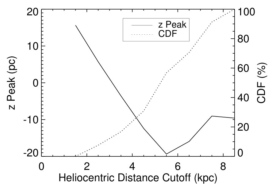 Figure 1
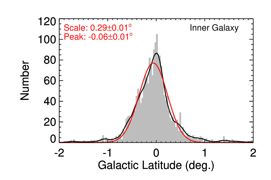 Figure 2
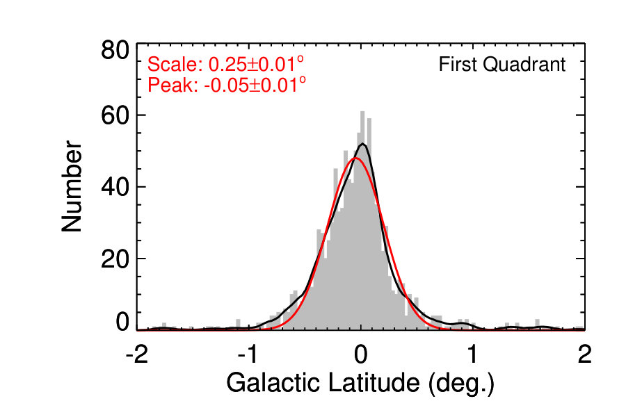 Figure 3
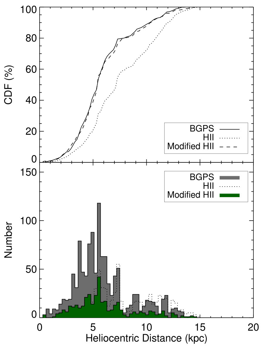 Figure 4
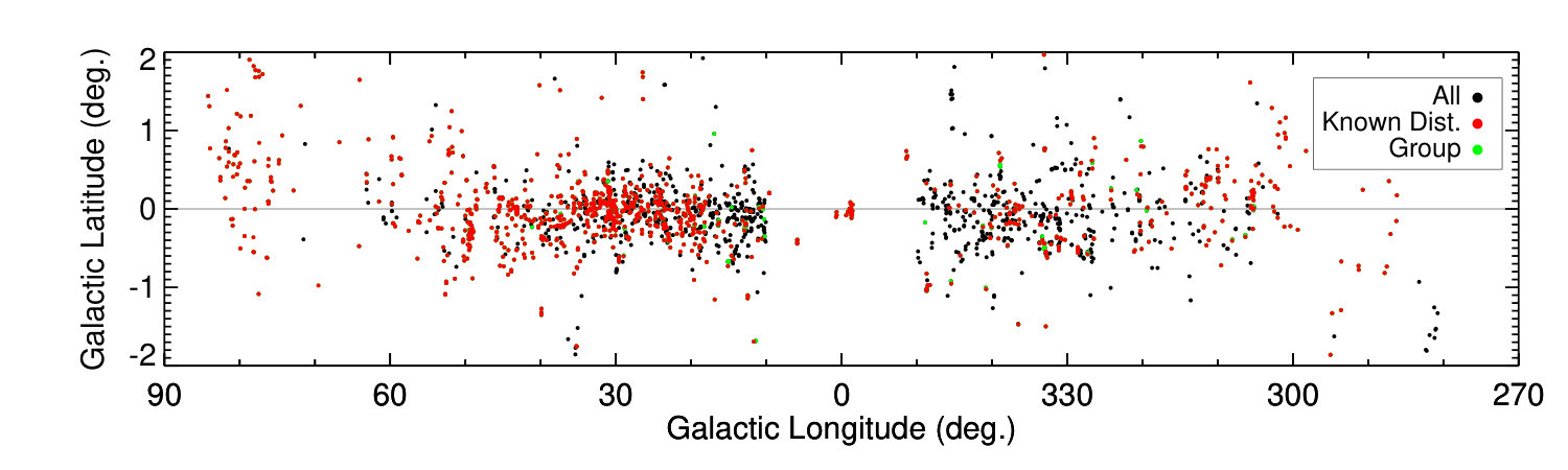 Figure 5
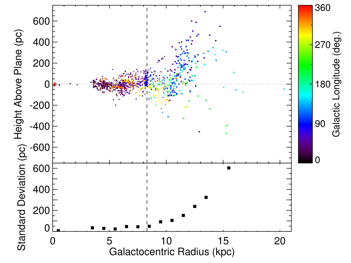 Figure 6
 Figure 7
 Figure 8
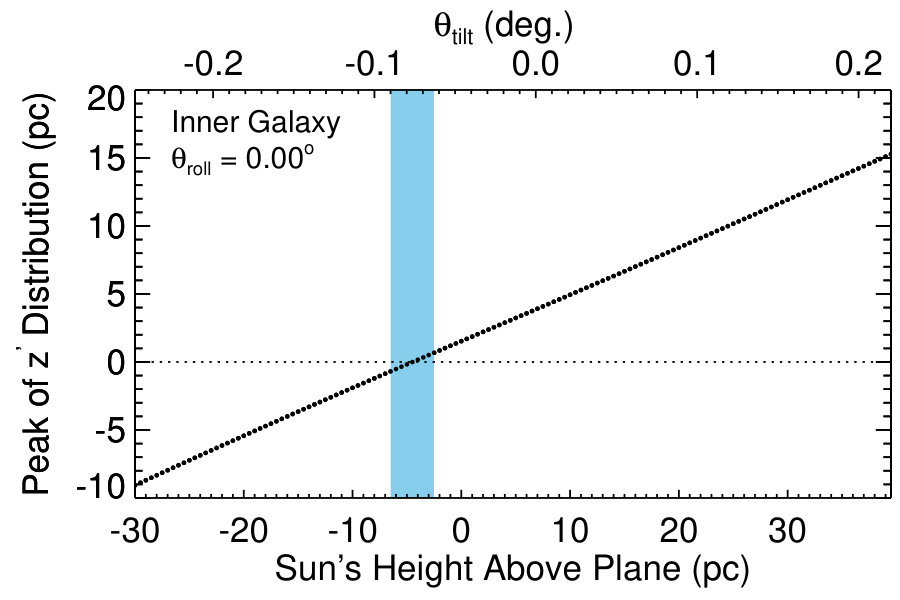 Figure 9
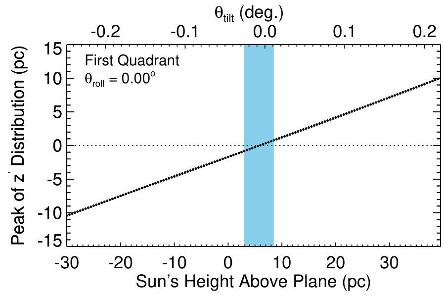 Figure 10
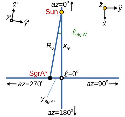 Figure 11
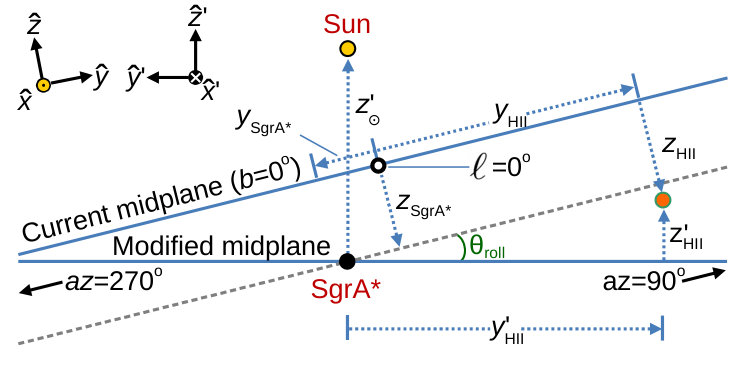 Figure 12
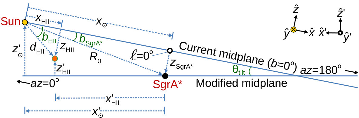 Figure 13
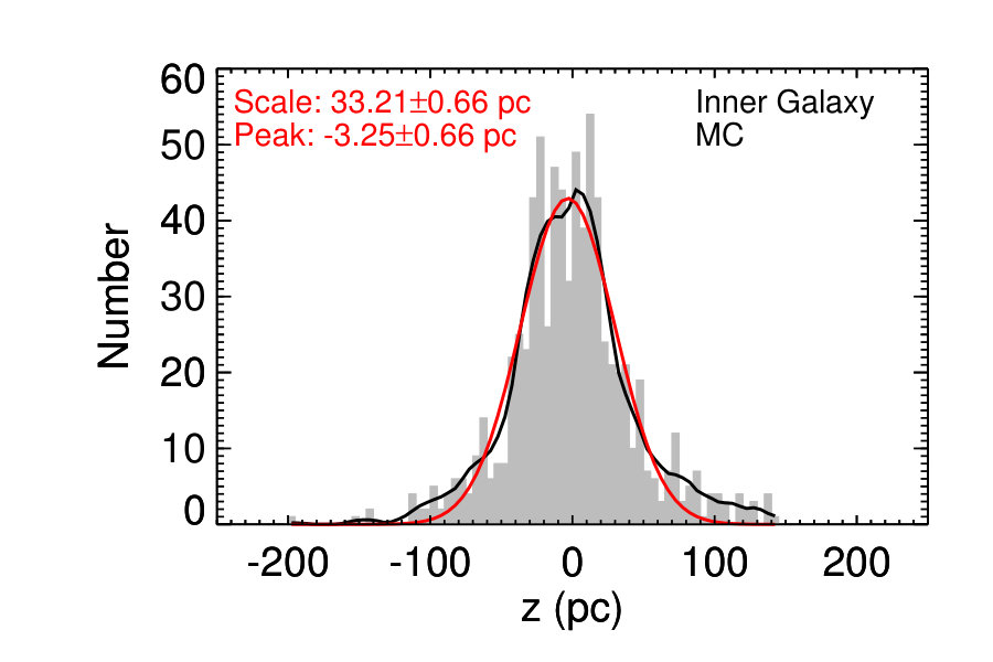 Figure 14
 Figure 15
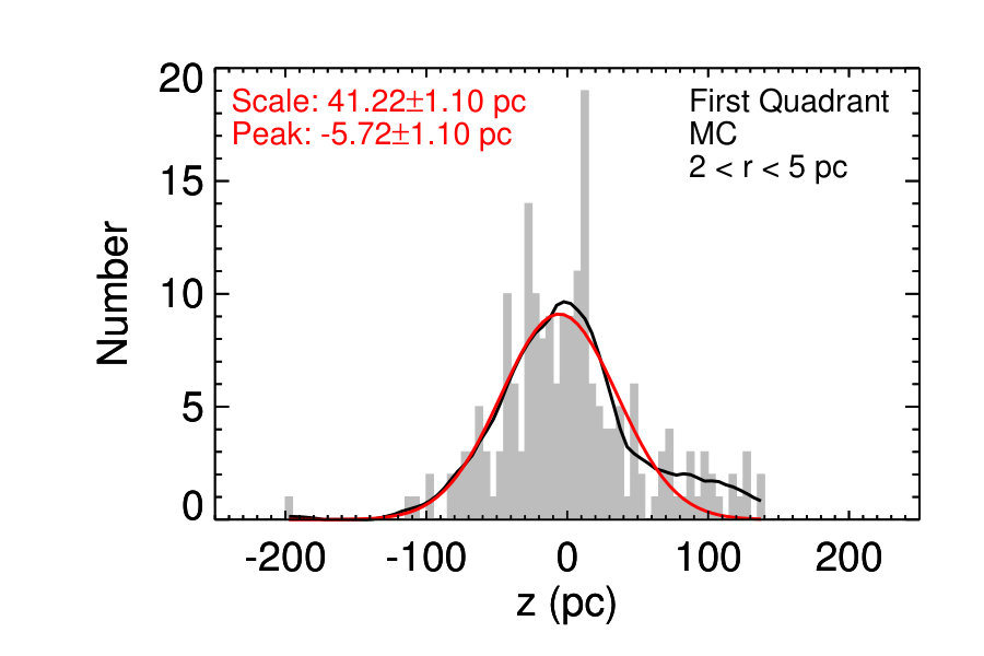 Figure 16
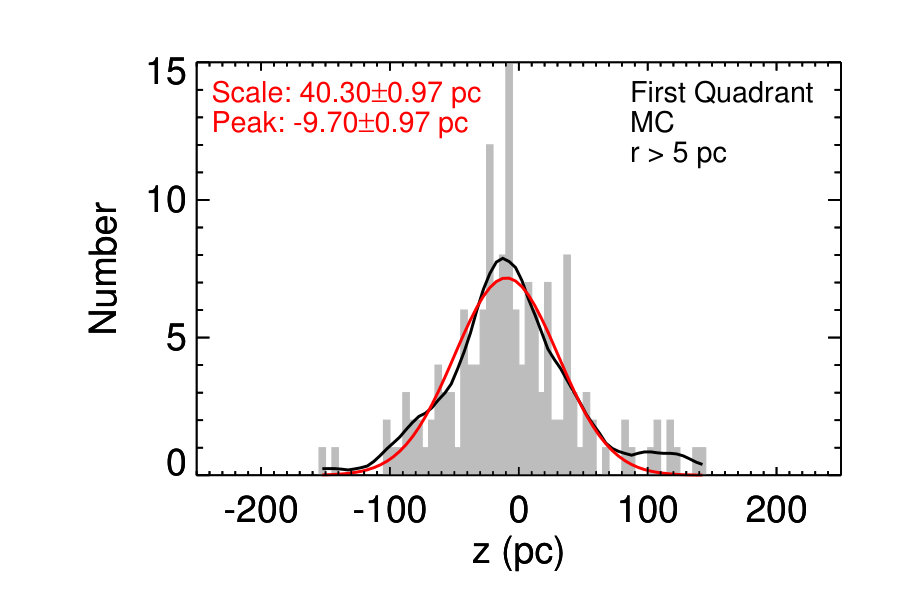 Figure 17
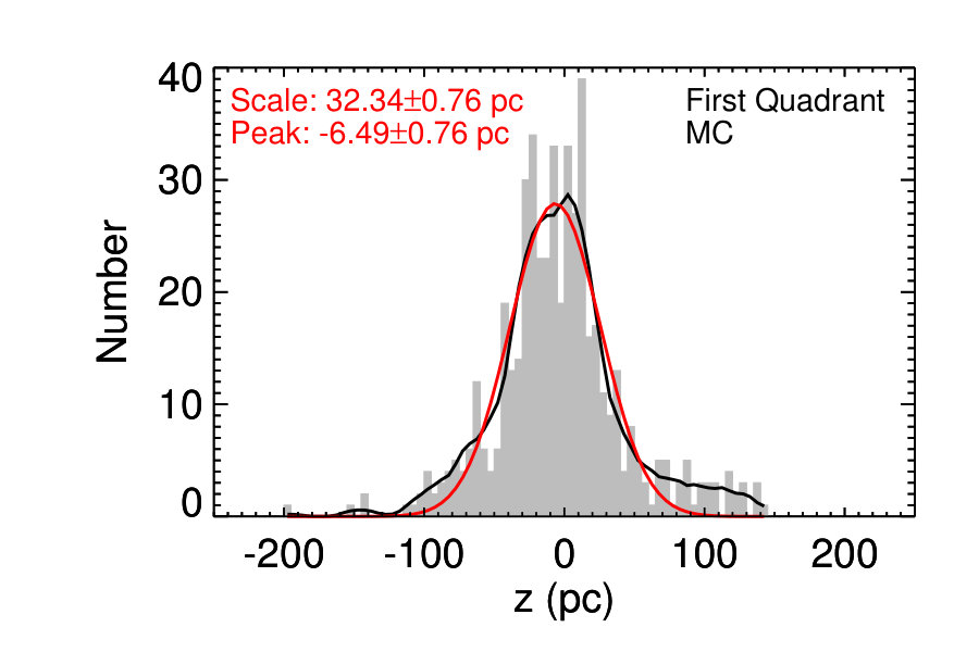 Figure 18
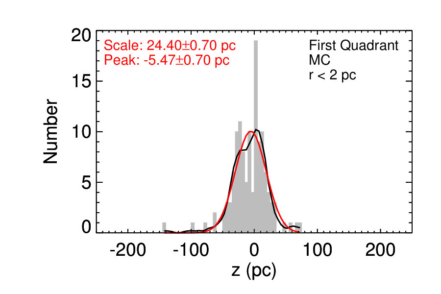 Figure 19
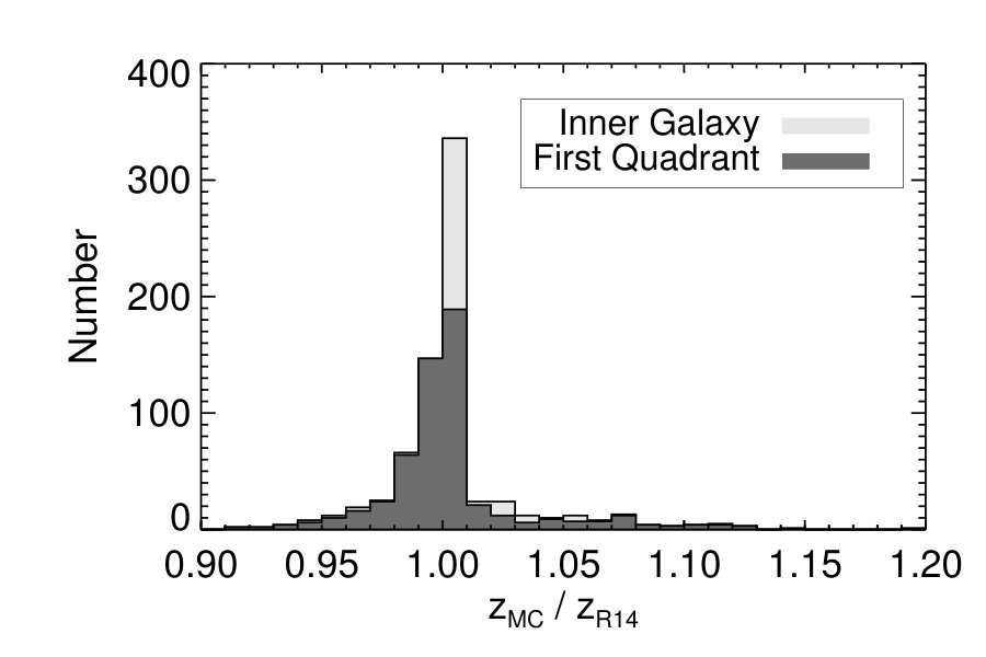 Figure 20
| Tracer | Galactic Latitude | Height | |||||
| Scale Heighta | Peak | Scale Heighta | Peak | Zone | Referenceb | ||
| (deg.) | (deg.) | (pc) | (pc) | ||||
| ATLASGAL 870 µm cont. | 1 | ||||||
| ATLASGAL 870 µm cont. | 2 | ||||||
| ATLASGAL 870 µm cont. | 2 | ||||||
| ATLASGAL 870 µm cont. | 0 | 2 | |||||
| BGPS 1.1 mm cont. | 3 | ||||||
| BGPS 1.1 mm cont. | 4c | ||||||
| IR-identified star clusters | Entire Galaxy | 5 | |||||
| Ultra-compact HII regions | Entire Galaxy | 6 | |||||
| Ultra-compact HII regions | 31 | 7 | |||||
| Ultra-compact HII regions | 0.6 | 30 | Entire Galaxy | 8 | |||
| HII regions | 42 | 9 | |||||
| HII regions | 39.3 | 7.3 | Entire Galaxy, | 10d | |||
| HII regions | 7.6 | Entire Galaxy, | 11e | ||||
| High mass star forming regions | to 0 | 12 | |||||
| masers | 13 | ||||||
| HI cold neutral medium | Entire Galaxy | 14 | |||||
| CO | Entire Galaxy | 15 | |||||
| Far-IR dust | Entire Galaxy | 16 | |||||
| Far-IR dust | 17 | ||||||
| 158 µm [CII] | 73 | Entire Galaxy at | 18 | ||||
| Location | Sun-centered | Sgr A∗-centered |
|---|---|---|
| Sun: (—,—,0) | ||
| Sgr A∗: | ||
| Current GC: |
| Galactic Latitude | Height | |||||||
| Sample | Rot. Curve | Modification | Number | Scale Height | Peak | Number | Scale Height | Peak |
| (deg.) | (deg.) | (pc) | (pc) | |||||
| First Quadrant | MC | 682 | 458 | |||||
| First Quadrant | MC | Unique | 605 | 408 | ||||
| First Quadrant | MC | Group | 1132 | 725 | ||||
| First Quadrant | R14 | 682 | 475 | |||||
| First Quadrant | B93 | 682 | 475 | |||||
| Inner Galaxy | MC | 1149 | 613 | |||||
| First Quadrant | MC | 130 | 104 | |||||
| First Quadrant | MC | 211 | 200 | |||||
| First Quadrant | MC | 159 | 154 | |||||
| Free | |||||||||
| Sample | Rot. Curve | Modification | Number | ||||||
| (pc) | (deg.) | (pc) | (deg.) | (deg.) | |||||
| First Quadrant | MC | 458 | - | ||||||
| First Quadrant | MC | Unique | 408 | 0.02±0.01 | 6.5±0.8 | 0.00±0.01 | |||
| First Quadrant | MC | Group | 725 | 0.01±0.01 | 9.4±0.6 | 0.02±0.01 | |||
| First Quadrant | R14 | 475 | 0.01±0.01 | 4.2±1.1 | 0.02±0.01 | 0.03±0.01 | |||
| First Quadrant | B93 | 475 | 0.01±0.01 | 5.7±1.2 | 0.01±0.01 | 0.04±0.01 | |||
| Inner Galaxy | MC | 613 | 0.07±0.01 | 1.3±0.4 | 0.04±0.01 | 0.04±0.01 | |||
| First Quadrant | MC | 306 | 0.01±0.02 | ||||||
| First Quadrant | MC | 385 | 0.02±0.02 | 15.0±0.6 | 0.06±0.01 | 0.05±0.01 | |||
| First Quadrant | MC | 441 | 0.00±0.02 | 14.3±0.7 | 0.05±0.01 | 0.09±0.01 | |||
| First Quadrant | MC | 104 | 0.04±0.01 | 3.3±1.3 | 0.07±0.01 | 0.04±0.01 | |||
| First Quadrant | MC | 200 | 0.02±0.02 | 18.0±1.2 | 0.08±0.01 | 0.15±0.01 | |||
| First Quadrant | MC | 154 | 0.08±0.03 | 8.6±1.5 | 0.11±0.01 | 0.02±0.01 | |||
Peer Reviews
No public reviews on file for this paper yet. If you reviewed it on a platform where reviews are public (OpenReview, ICLR, NeurIPS, ICML), you can paste yours below so the community can read it here.
Videos
No videos yet. Explain this paper in a talk, walkthrough, or lecture? Add one.
A Galactic Plane Defined by the Milky Way H II Region Distribution
L. D. Anderson
Department of Physics and Astronomy, West Virginia University, Morgantown WV 26506, USA
Adjunct Astronomer at the Green Bank Observatory, P.O. Box 2, Green Bank WV 24944, USA
Center for Gravitational Waves and Cosmology, West Virginia University, Chestnut Ridge Research Building, Morgantown, WV 26505, USA
Trey V. Wenger
Astronomy Department, University of Virginia, P.O. Box 400325, Charlottesville, VA 22904-4325, USA
W. P. Armentrout
Department of Physics and Astronomy, West Virginia University, Morgantown WV 26506, USA
Center for Gravitational Waves and Cosmology, West Virginia University, Chestnut Ridge Research Building, Morgantown, WV 26505, USA
Green Bank Observatory, P.O. Box 2, Green Bank WV 24944, USA
Dana S. Balser
National Radio Astronomy Observatory, 520 Edgemont Road, Charlottesville VA, 22903-2475, USA
T. M. Bania
Institute for Astrophysical Research, Department of Astronomy, Boston University, 725 Commonwealth Ave., Boston MA 02215, USA
Abstract
We develop a framework for a new definition of the Galactic midplane, allowing for tilt (; rotation about Galactic azimuth ), and roll (; rotation about Galactic azimuth ) of the midplane with respect to the current definition. Derivation of the tilt and roll angles also determines the solar height above the midplane. Here we use nebulae from the WISE Catalog of Galactic H II Regions to define the Galactic high-mass star formation (HMSF) midplane. We analyze various subsamples of the WISE catalog and find that all have Galactic latitude scale heights near and -distribution scale heights near 30 . The vertical distribution for small (presumably young) H II regions is narrower than that of larger (presumably old) H II regions ( versus ), implying that the larger regions have migrated further from their birth sites. For all H II region subsamples and for a variety of fitting methodologies, we find that the HMSF midplane is not significantly tilted or rolled with respect to the currently-defined midplane, and therefore the Sun is near to the HMSF midplane. These results are consistent with other studies of HMSF, but are inconsistent with many stellar studies, perhaps due to asymmetries in the stellar distribution near the Sun. Our results are sensitive to latitude restrictions, and also to the completeness of the sample, indicating that similar analyses cannot be done accurately with less complete samples. The midplane framework we develop can be used for any future sample of Galactic objects to redefine the midplane.
Galaxy: structure – ISM: H II regions
1 Introduction
The midplane, the plane at Galactic latitude , was defined in 1958 by the IAU subcommission 33b, which set the Galactic coordinate system (Blaauw et al., 1960). The IAU midplane definition comes from the Galactic Center location in B1950 coordinates of (17:42:26.6, 28:55:00) and the north Galactic pole location in B1950 coordinates of (12:49:00, +27:24:00). Ideally, the midplane definition would contain the minimum of the Galactic potential and there would be equal amounts of material above and below the midplane. The vertical distribution of objects with respect to the Galactic midplane tells us fundamental parameters of Galactic structure, such as the scale height of the objects studied, the Sun’s height above or below the midplane, , and even the orientation of the midplane itself. Nearly all previous studies of the vertical distribution of objects in the Galaxy have found an asymmetry in the distribution of sources above and below the plane, with more sources found below the IAU plane than above it. This asymmetry is generally assumed to be the result of the Sun’s location above the IAU Galactic midplane.
Previous studies of the vertical distribution of objects and solar height above the plane can be categorized as either using stellar or gas samples. Solar height studies are summarized in Humphreys & Larsen (1995) and Karim & Mamajek (2017). Studies of stellar samples have a long history; perhaps the first such study was done by van Tulder (1942), who found an asymmetry in the stellar distribution that implied that the Sun is pc above the plane. Typical stellar studies examine discrepancies in the number of sources toward the north and south Galactic poles to determine the solar height (e.g., Humphreys & Larsen, 1995). A typical value for the solar height from stellar studies is 20 pc; for example, Maíz-Apellániz (2001) used OB stars from to derive pc, Chen et al. (2001) used stars from an early release of the Sloan Digital Sky Survey (SDSS) to derive pc., and Jurić et al. (2008) found using SDSS data release 3 (with some data release 4) that the -distributions for stars of a range of colors and brightnesses are all consistent with pc.
We summarize the studies of Galactic latitude and -distributions that use gas tracers in Table 1, focusing on works that use tracers sensitive to HMSF. This table contains the peak and scale height of the distributions. If the fits were exponential, we list the stated scale height. If the fits were Gaussians, we list the scale height as
[TABLE]
where FWHM is the full width at half maximum of the distribution. For a given sample, we do not expect significant discrepancies between the exponential and Gaussian scale heights (Bobylev & Bajkova, 2016). There are larger discrepancies between values derived using gas tracers compared to those derived using stellar tracers. There is, nevertheless, good agreement that the various distributions peak below the Galactic midplane. The tracers that are most sensitive to HMSF have narrow distributions with scale heights , whereas the distributions of H I, CO, far-infrared emitting dust, and C II are broader.
The solar height above the plane derived using gas tracers is generally lower than that found from stellar tracers (see compilation in Karim & Mamajek, 2017). Typical values are near 10 . For example, Bobylev & Bajkova (2016) found from a sample of H II regions, masers, and molecular clouds and Paladini et al. (2003) found using a sample of H II regions.
Because it was defined using low-resolution data and our measurements have since improved significantly, the IAU-defined Galactic midplane may need to be revised (Goodman et al., 2014). We now know that Sgr A∗ lies at (Reid & Brunthaler, 2004), which places it below the IAU-defined location of the Galactic Center (although by the IAU’s definition Sgr A is at the Galactic center (Blaauw et al., 1960)). Goodman et al. (2014) investigated the implications of this offset and of the Sun lying above the midplane using the extremely long “Nessie” infrared dark cloud (IRDC). Although Nessie lies below the midplane as it is currently defined, because of the Sun’s offset and the offset of Sgr A∗ from , they found that Nessie may actually lie in what they call the “true” midplane, which is tilted by angle with respect to the IAU midplane definition111We call this rotation the “tilt” angle to be consistent with previous authors, although by convention it would be called the “pitch” angle.. While suggestive, this study needs to be expanded to a larger sample of objects in order to make stronger claims about the midplane definition.
Tracers of HMSF formation should define the Galactic midplane, although it is difficult to create a large, unbiased sample of HMSF regions. Most of the gas tracers are related to massive stars, which are born in the most massive molecular clouds in the Galaxy. The high-mass stars themselves have lifetimes short enough that they are unable to travel far from their birthplaces. For example, an O-star with a space velocity of 10 can only travel 100 pc out of the midplane in 10 Myr, and only then if its velocity is entirely in the direction. Other tracers of high-mass stars should be similarly restricted to the midplane.
In Section 2, we first develop the methodology needed to redefine the Galactic midplane. We apply this methodology to the WISE Catalog of Galactic H II Regions (Anderson et al., 2014) in Section 4, after first characterizing the vertical structure of the Galaxy’s H II region population in Section 3. We therefore define the HMSF midplane, determine the tilt and roll angles of the HMSF midplane with respect to the current IAU definition and determine the Sun’s displacement from the HMSF midplane. The WISE catalog does not suffer from the same incompleteness and biases of other studies, and so may be better suited to determining the HMSF midplane than tracers used previously.
2 Defining the Galactic Midplane
Here, we develop the methodology required to define the midplane using a sample of discrete Galactic objects. Although the derived equations are general, we assume in later sections that the midplane passes through Sgr A∗. Future analyses with more data points may be able to relax this assumption.
2.1 Coordinate systems
To define the Galactic midplane, we need to use two coordinate systems: the current IAU Galactic coordinate system centered on the Sun (, , and ) and a new one centered on Sgr A∗ using the “modified” midplane definition. A Galactic azimuth () of zero degrees connects the Sun and the Galactic Center, and azimuth increases clockwise in the plane as viewed from the north Galactic pole.222Technically, is different between the two coordinate systems. We use here the azimuth defined in the current coordinate system, but only to orient the reader. In the Sun-centered coordinates, points from the Sun to the (currently-defined) Galactic center, points in the direction of Galactic azimuth , and points toward the Galactic north pole. In the Sgr A∗-centered coordinate system, points from Sgr A∗ in the approximate direction of the Sun, points in the direction of Galactic azimuth , and points approximately toward the Galactic north pole.
We show the geometries of the two coordinate systems in Figures 1, 2, and 3. The modified midplane can be tilted by angle (rotated about ; Figure 2) and rolled by angle (rotated about ; Figure 3). The modified midplane takes the form
[TABLE]
Sgr A∗ is located at (Reid & Brunthaler, 2004), which gives non-zero values for and . As can be seen in Figure 2,
[TABLE]
We can use the geometries in Figures 1 and 3 to determine
[TABLE]
We derive conversions between these coordinate systems in Appendix A, with the main result being the derivation of :
[TABLE]
where
[TABLE]
We can therefore compute for each Galactic object, given its values, the rotation angles, and the location of Sgr A∗. We give the -heights for locations along in Table 2.
2.1.1 Midplane tilt, midplane roll, and the Sun’s height
The tilt angle, which is apparent in Figure 2, does not have a compact analytical form unless we make some simplifying assumptions. Its complete form can be found by solving (cf. Appendix A):
[TABLE]
To simplify the equation for , we assume that (Goodman et al., 2014, find ), so . We can further assume that so that and is small compared to the other terms. The tilt angle is then:
[TABLE]
This differs from the angle used in Ellsworth-Bowers et al. (2013) by the additional term .
The roll angle is apparent in Figure 3. There is no compact solution for under reasonable assumptions. Its full form can be found by solving Equation A8.
3 The WISE Catalog of Galactic HII Regions
We wish to investigate the HMSF midplane using H II regions in the WISE Catalog of Galactic H II Regions (hereafter the WISE catalog Anderson et al., 2014), which contains all known Galactic H II regions. First, however, we characterize this sample of H II regions, and define subsamples to investigate how results may change when smaller numbers of H II regions are used. We use V2.1 of the WISE catalog333http://astro.phys.wvu.edu/wise/, which contains 1813 known H II regions that have ionized gas spectroscopic observations, 1130 of which have known distances. This H II region sample extends across the entire Galactic disk to Heliocentric distances kpc and Galactocentric distances kpc (Anderson et al., 2015). Since the WISE catalog was derived using -resolution 12 µm data, or Spitzer data in crowded fields, and the nominal H II region size is on the order of arcminutes, confusion is minimal. Therefore, the WISE catalog suffers less from blending of distant regions compared with lower resolution studies (see Beuther et al., 2012). The catalog also has no latitude restriction, which removes an additional impediment to the study of the vertical distribution of HMSF (see Section 4.4.3).
We compute the height above the plane, , for each WISE catalog H II region using Equation 6:
[TABLE]
where is the Heliocentric distance and latitude from the nominal H II region centroid position in the catalog. The definition of has no correction for the Sun’s height above the midplane, and so differs from that used in some recent studies (e.g., Ellsworth-Bowers et al., 2015). There is also no correction for the displacement of Sgr A∗ below .
If available, the catalog distances are from maser parallax measurements (e.g., Reid et al., 2009, 2014), but otherwise they are kinematic distances. The original WISE catalog used the Brand & Blitz (1993, hereafter B93) rotation curve for kinematic distances. Here, we update all known H II region distances using the method of Wenger et al. (2018, hereafer “MC”), which better accounts for uncertainties in kinematic distances. Because of their large uncertainties, the catalog contains no kinematic distances for H II regions within in Galactic longitude of the Galactic Center, within of the Galactic anti-center, and for any region where the distance uncertainty is . We use throughout (Reid et al., 2014).
Because of the Galactic warp, we cannot use all cataloged H II regions to investigate vertical structure in the Galaxy. The warp is known to begin around the solar orbit (Clemens et al., 1988), at kpc. We investigate the warp by plotting the distribution of H II regions as a function of in the top panel of Figure 4. Each point in the top panel of Figure 4 represents an H II region, color-coded by its Galactic longitude. In agreement with previous results, the warp as traced by H II regions begins near the solar circle () and extends toward the north Galactic pole in the first Galactic quadrant and toward the south Galactic pole in the third Galactic quadrant.
The standard deviation of the H II region sample shown in the bottom panel of Figure 4 is relatively constant in the inner Galaxy. The inner Galaxy values are all and this can be thought of as the scale height. In the outer Galaxy, the standard deviation increases with Galactocentric radius as a result of the Galactic warp. This agrees with the results of the H II region study by Paladini et al. (2004) and the CO study by Malhotra (1994). We exclude bins that have fewer than 10 sources from these computations.
In the analysis of the HMSF midplane (Section 4), we exclude sources with , where . We also exclude regions with distance uncertainties . We show the Galactic locations of the H II regions studied here in Figure 5. The lack of regions within of the Galactic Center is in part caused by a lack of known distances for those regions. Most regions in the large concentration near are associated with the Cygnus X complex.
3.1 Subsamples of the WISE Catalog
Due to issues of completeness and biases introduced by large H II region complexes, we define multiple subsamples of the WISE catalog. We run our analyses on these subsamples to investigate potential biases in our results. We also test the impact of using different rotation curve models. For all subsamples, we include only regions with , with .
3.1.1 Galactic Quadrants
The completeness of the WISE catalog varies across the Galaxy. Nearly all recent H II region surveys have taken place in the northern sky, and therefore there are many more known H II regions in the first Galactic quadrant compared to the fourth. The luminosity distribution of the first quadrant sample suggests that it is complete for all H II regions ionized by single O-stars, but this is not the case in the fourth quadrant (W. Armentrout et al., 2018, in prep.). This asymmetry may introduce a bias into our analysis. We therefore perform our analyses below using two Galactic longitude subsamples that both have : one from (hereafter the “first quadrant sample”) and one containing all regions in the first and fourth quadrants (the “inner Galaxy sample”). The first quadrant sample has 682 H II regions, 458 of which have known distances, and the inner Galaxy sample has 1149 H II regions, 613 of which have known distances.
3.1.2 HII Region Complexes
H II regions are frequently found in large complexes containing many individual H II regions. The WISE catalog lists entries for each individual region in the complex and therefore the results of a statistical study will differ based on whether the complex is considered to be one H II region or many. There are objects in the WISE catalog that do not have ionized gas or molecular spectroscopic observations, but are placed into a complex on the basis of the appearance of the complex in mid-infrared and radio continuum data (e.g., W49, W51, Sgr B2, etc.). The distance to these regions are assumed to be that of the other complex members. These large complexes may bias our results because there are many regions in the catalog at particular Galactic locations. This bias may be warranted because these large complexes may better define the midplane (as found by V. Cunningham et al., 2018, in prep.).
We test for the effect of complexes on our results by running the analyses on two subsamples, one only containing “unique” H II regions (i.e., each complex contains only one catalog entry), and the other that has all regions, including “group” regions that that are in large H II region complexes but which lack individual spectroscopic observations. For the group regions, we assume the kinematic distance of the other complex members. We only show results from these subsamples in the first Galactic quadrant. In the first Galactic quadrant, the unique subsample contains 605 H II regions, 408 of which have known distances, and the group subsample contains 1132 H II regions, 725 of which have known distances.
3.1.3 Rotation Curves
The majority of the WISE catalog distances are kinematic, and are therefore sensitive to the choice of rotation curve. Different distances result in different values for (cf. Equation 8). We examine how our results change when kinematic distances are computed using the B93 curve, the Reid et al. (2014, hereafter “R14”), and the MC analysis. We do not change the parallax distances in any of our trials. R14 lists multiple rotation curve models; the one we use here has a solar circular angular velocity , a solar distance from the Galactic Center , and . In general, the B93 curve gives larger distances compared to the R14 curve, and therefore the B93 - distances are larger than those of R14 (Figure 6, top panel). The MC and R14 curve -distances are similar (Figure 6, bottom panel).
3.2 Characterizing the HII Region Vertical Distribution
We characterize the WISE catalog Galactic latitude distribution for all H II regions in the sample and the -distribution for regions with known distances in Table 3. These analyses do not rely on the modified midplane definition in Section 2, but are comparable to those derived by previous authors in Table 1.
3.2.1 Galactic Latitude Distribution
The distribution of Galactic latitudes is representative of the -height distribution, but since it does not require distances to the objects the analysis can be done on a larger sample of H II regions. Figure 7 shows the first quadrant and inner Galaxy H II region Galactic latitude distributions, although we perform the same analysis for all subsamples defined previously, for all rotation curves. We plot the “kernel density estimation” (KDE) in the black curve. The KDE estimates the underlying distribution, and an analysis of the KDE is free from the uncertainties associated with the choice of bin size. For this and all subsequent analyses, we use the “Epanechnikov” kernel with the optimal bandwidth as suggested by Silverman (1986, their Equation 3.31). We fit the KDE distributions with Gaussian functions and store the results in Table 3.
For all subsamples, the peak of the Galactic latitude distribution is slightly below (possibly indicating a positive value for the solar height ), ranging from to . The scale height, again the standard deviation of a Gaussian fit to the Galactic latitude distribution, is between and for all subsamples. These scale height values are similar to those found for other high-mass star tracers (Table 1). It is interesting that our sample of H II regions, which spans a wide range of evolutionary stages, has the same scale height as tracers that are more sensitive to future star formation (e.g., sub-mm/mm clumps). We can infer that the lifetime of H II regions is short enough to not make a large difference in their -distribution compared with younger objects.
3.2.2 -Distribution
For regions with known distances, we can study the -height distribution directly. The -distributions, for which we show examples in Figure 8, are approximately Gaussian for all subsamples. There are, however, “wings” to the distributions at high and low values of . As with the Galactic latitude distributions, we fit the KDEs of the distributions with Gaussian functions and store the results in Table 3. The analysis of the z-distribution is necessarily limited to only H II regions with known distances, which is a smaller subsample compared to that used in the Galactic latitude analysis. All subsamples peak at small negative values, from to , again implying that the Sun is located above the midplane. The scale heights for the various subsamples range from to . All distance methods return similar results. These values are similar to those found for ultra-compact H II regions (Bronfman et al., 2000), sub-mm clumps (Wienen et al., 2015) and high-mass star forming regions (Urquhart et al., 2011) (see Table 1).
3.2.3 Variations with HII Region Size
Finally, we test how the - and -distributions changes when the sample is restricted to H II regions of various physical sizes. The size of an H II region is a proxy for its age (e.g. Spitzer, 1978). Diffuse H II regions are difficult to detect (Lockman et al., 1996; Anderson et al., 2017), and excluding larger diffuse regions from the sample may have an impact on the derived results. We divide the first quadrant sample into three physical size groups based on the WISE catalog radius : , , and . We show these distributions and fits in Figure 9, and give the fit parameters in Table 3. Smaller regions have a smaller scale height of , whereas the largest regions have scale heights of . Furthermore, the larger region distributions are consistent with larger solar heights and hence larger tilt angles. Assuming the smaller regions are on average younger, this result is consistent with migration of older regions out of the plane as they age.
The reference list from the paper itself. Each links out to its DOI / PubMed record.
- 1Anderson et al. (2015) Anderson, L. D., Armentrout, W. P., Johnstone, B. M., et al. 2015, Ap JS, 221, 26
- 2Anderson et al. (2017) Anderson, L. D., Armentrout, W. P., Luisi, M., et al. 2017, Ar Xiv e-prints, ar Xiv:1710.07397
- 3Anderson & Bania (2009) Anderson, L. D., & Bania, T. M. 2009, Ap J, 690, 706
- 4Anderson et al. (2014) Anderson, L. D., Bania, T. M., Balser, D. S., et al. 2014, Ap JS, 212, 1
- 5Becker et al. (1994) Becker, R. H., White, R. L., Helfand, D. J., & Zoonematkermani, S. 1994, Ap JS, 91, 347
- 6Beichman et al. (1988) Beichman, C. A., Neugebauer, G., Habing, H. J., Clegg, P. E., & Chester, T. J., eds. 1988, Infrared astronomical satellite (IRAS) catalogs and atlases. Volume 1: Explanatory supplement, Vol. 1
- 7Beuther et al. (2012) Beuther, H., Tackenberg, J., Linz, H., et al. 2012, Ap J, 747, 43
- 8Blaauw et al. (1960) Blaauw, A., Gum, C. S., Pawsey, J. L., & Westerhout, G. 1960, MNRAS, 121, 123