Numerical analysis of dynamical systems: unstable periodic orbits, hidden transient chaotic sets, hidden attractors, and finite-time Lyapunov dimension
N.V. Kuznetsov, T.N. Mokaev

TL;DR
This paper discusses the challenges of numerically analyzing chaotic dynamical systems, focusing on hidden attractors, transient chaos, and finite-time Lyapunov dimensions using classic models like Lorenz, Rossler, and Vallis.
Contribution
It introduces methods for detecting hidden attractors and accurately computing finite-time Lyapunov exponents and dimensions in low-order chaotic models.
Findings
Identification of hidden chaotic attractors in Lorenz system.
Demonstration of finite-time Lyapunov dimension computation.
Analytical localization of attractors in Vallis system.
Abstract
In this article, on the example of the known low-order dynamical models, namely Lorenz, Rossler and Vallis systems, the difficulties of reliable numerical analysis of chaotic dynamical systems are discussed. For the Lorenz system, the problems of existence of hidden chaotic attractors and hidden transient chaotic sets and their numerical investigation are considered. The problems of the numerical characterization of a chaotic attractor by calculating finite-time time Lyapunov exponents and finite-time Lyapunov dimension along one trajectory are demonstrated using the example of computing unstable periodic orbits in the Rossler system. Using the example of the Vallis system describing the El Nino-Southern Oscillation it is demonstrated an analytical approach for localization of self-excited and hidden attractors, which allows to obtain the exact formulas or estimates of their Lyapunov…
Click any figure to enlarge with its caption.
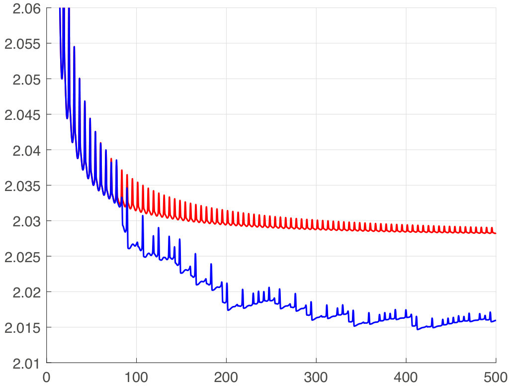 Figure 1
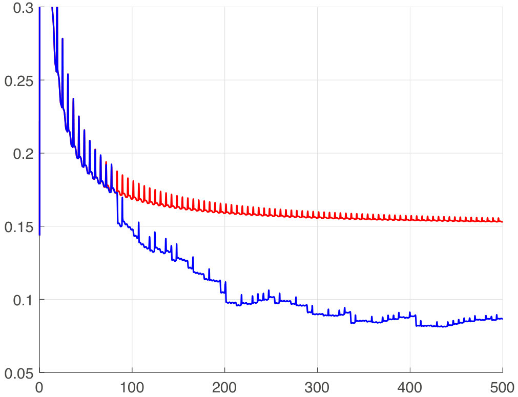 Figure 2
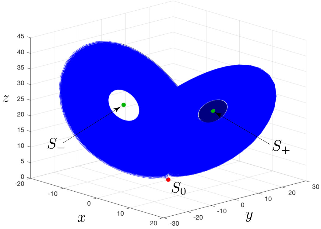 Figure 3
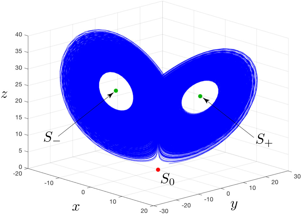 Figure 4
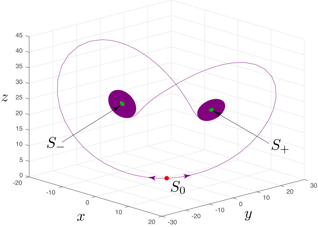 Figure 5
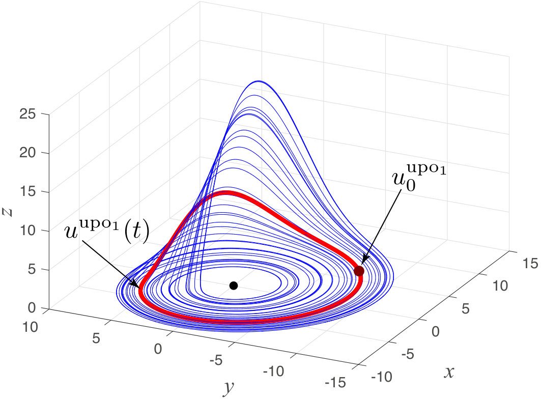 Figure 6
Peer Reviews
No public reviews on file for this paper yet. If you reviewed it on a platform where reviews are public (OpenReview, ICLR, NeurIPS, ICML), you can paste yours below so the community can read it here.
Videos
No videos yet. Explain this paper in a talk, walkthrough, or lecture? Add one.
Numerical analysis of dynamical systems: unstable periodic orbits,
hidden transient chaotic sets, hidden attractors, and finite-time Lyapunov dimension
N. V. Kuznetsov
Corresponding author: [email protected]
Faculty of Mathematics and Mechanics, St. Petersburg State University, Peterhof, St. Petersburg, Russia
Department of Mathematical Information Technology, University of Jyväskylä, Jyväskylä, Finland
Institute of Problems of Mechanical Engineering RAS, Russia
T. N. Mokaev
Faculty of Mathematics and Mechanics, St. Petersburg State University, Peterhof, St. Petersburg, Russia
Abstract
In this article, on the example of the known low-order dynamical models, namely Lorenz, Rössler and Vallis systems, the difficulties of reliable numerical analysis of chaotic dynamical systems are discussed. For the Lorenz system, the problems of existence of hidden chaotic attractors and hidden transient chaotic sets and their numerical investigation are considered. The problems of the numerical characterization of a chaotic attractor by calculating finite-time time Lyapunov exponents and finite-time Lyapunov dimension along one trajectory are demonstrated using the example of computing unstable periodic orbits in the Rössler system. Using the example of the Vallis system describing the El Ninõ-Southern Oscillation it is demonstrated an analytical approach for localization of self-excited and hidden attractors, which allows to obtain the exact formulas or estimates of their Lyapunov dimensions.
I Introduction
History of the turbulence phenomena study is associated with the consideration of various models, which include the Navier-Stokes equations, their Galerkin approximations, and the development of the theory of chaos Landau-1944 ; Hopf-1948 ; RuelleT-1971 ; Smale-1967 . Here let us note the significant results by D. Ruelle, F. Takens RuelleT-1971 , and S. Smale Smale-1967 , who proposed a chaotic attractor as a mathematical prototype describing the onset of turbulence, and by O. Ladyzhenskaya, who studied the case when the two-dimensional Navier-Stokes equation generates a dynamical system and proved the finite dimensionality of its attractor Ladyzhenskaya-1982 . The first vivid example of chaotic attractor in a hydrodynamic system was obtained by E. Lorenz Lorenz-1963 . Using the Galerkin method he derived a crude three-dimensional mathematical model for Rayleigh-Bénard convective flow, which has the following form:
[TABLE]
where , , are positive parameters. For , there is one globally asymptotically stable equilibrium . For , equilibrium is a saddle, and a pair of symmetric equilibria appears.
For the parameters , , in system (1) E. Lorenz numerically found a chaotic attractor in the model. In general, for numerical localization of attractor, it is necessary to explore its basin of attraction and choose an initial point in it. If for a particular attractor its basin of attraction is connected with the unstable manifold of unstable equilibrium, then the localization procedure is quite simple. From this perspective, the following classification of attractors is suggested LeonovKV-2011-PLA ; LeonovK-2013-IJBC ; LeonovKM-2015-EPJST ; Kuznetsov-2016 : an attractor is called a self-excited attractor if its basin of attraction intersects an arbitrarily small open neighborhood of an equilibrium; otherwise, it is called a hidden attractor. Numerical localization of hidden attractors is much more challenging and requires the development of special methods. The classical Lorenz attractor is a self-excited one with respect to all equilibria , , and it is an open question (Kuznetsov-2016, , p. 14) whether for some parameters there exists a hidden Lorenz attractor. This question is related to the ’’chaotic’’ generalization LeonovK-2015-AMC of the second part of Hilbert’s 16th problem on the number and mutual disposition of attractors and repellers in the chaotic multidimensional dynamical systems and, in particular, their dependence on the degree of polynomials in the model; see corresponding discussion, e.g. in SprottJKK-2017 ; ZhangChen-2017 . There are a number of physical dynamical models which possess hidden chaotic attractors, e.g, the Rabinovich system (describes the interaction of plasma waves) KuznetsovLMPS-2018 ; ChenKLM-2017-IJBC , the Glukhovsky-Dolghansky system (describes convective fluid motion in a rotating cavity) LeonovKM-2015-CNSNS ; LeonovKM-2015-EPJST and others DancaKC-2016 ; DudkowskiJKKLP-2016 ; GarashchukSK-2018-HA ; GarashchukSK-2018-RCD .
We note that the Lorenz system (1) with parameters , , is dissipative in the sense of Levinson, and for any initial data (except for equilibria) the trajectory tends to the attractor. Thus, system (1) generates a dynamical system \big{(}\{\varphi^{t}\}_{t\geq 0},(U\subseteq\mathbb{R}^{3},||\cdot||)\big{)}.
II Hidden transient chaotic sets in Lorenz system
In numerical computation of a trajectory over a finite-time interval it is difficult to distinguish a sustained chaos from a transient chaos (a transient chaotic set in the phase space, which can nevertheless persist for a long time) GrebogiOY-1983 ; LaiT-2011 , thus it is reasonable to give a similar classification for transient chaotic sets DancaK-2017-CSF ; ChenKLM-2017-IJBC : a transient chaotic set is called a hidden transient chaotic set if it does not involve and attract trajectories from a small neighborhood of equilibria; otherwise, it is called self-excited. In order to distinguish an attracting chaotic set (attractor) from a transient chaotic set in numerical experiments, one can consider a grid of points in a small neighborhood of the set and check the attraction of corresponding trajectories towards the set. There one can reveal a subset of points for which the trajectories leave the transient set.
For the Lorenz system (1), suppose that , are fixed and varies. If , then all three equilibria , are unstable and in the phase space there exists a self-excited attractor with respect to these equilibria. For , the equilibria become stable, and for , there exists a self-excited attractor with respect to equilibrium . Near the point it is possible to observe a long living transient chaotic set, which is hidden since it’s basin of attraction does not intersect with the small vicinities of equilibrium . For example, for a hidden transient chaotic set can be visualized111 In this work, we use MATLAB’s standard procedure ode45 with default parameters. YuanYW-2017-HA from the initial point (see Fig. 1). In MunmuangsaenS-2018-HA , hidden transient chaotic set was obtained in system (1) with , , .
The time of the transient process in this case depends strongly on the choice of the initial data, which complicates the task of distinguishing an attracting chaotic set (attractor) from a transient chaotic set in numerical experiments. E.g., for system (1) with parameters , , and for initial point a transient chaotic behavior is observed222 The time of transient chaotic behavior is often estimated approximately by analyzing the sign of the largest Lyapunov exponent. For simplicity, here we approximate the transient behavior time by the time of entering a small ball with the center at the points . on the time interval , for initial point — on the time interval , for initial point — on the time interval , and for initial point a transient chaotic behavior continues over a time interval of more than . In order to distinguish an attracting chaotic set from a transient chaotic set by computing trajectories on a reasonable time interval, one can consider a grid of points in a small neighborhood of the set and check the attraction of corresponding trajectories towards the set. There one can reveal a subset of points for which the trajectories leave the transient set.
Next, on the example of the Lorenz system (1) we will demonstrate difficulties in the reliable numerical computation of the finite-time Lyapunov exponents and finite-time Lyapunov dimension.
III Finite-time Lyapunov dimension of a transient chaotic set
Consider system (1) with parameters , , and integrate numerically the trajectory with initial data . We numerically approximate the finite-time Lyapunov exponents and finite-time Lyapunov dimension (see corresponding definitions, e.g. in Kuznetsov-2016-PLA ; KuznetsovLMPS-2018 ). Integration with leads to the collapse of the ‘‘attractor’’, i.e. the ‘‘attractor’’ turns out to be a transient chaotic set. However, on the time interval we have and, thus, may conclude that the behavior is chaotic, and for the time interval we have . This effect is due to the fact that the finite-time Lyapunov exponents and finite-time Lyapunov dimension are the values averaged over the considered time interval. Since the lifetime of transient chaotic process can be extremely long and taking into account the limitations of reliable integration of chaotic ODEs, even long-time computation of the finite-time Lyapunov exponents and the finite-time Lyapunov dimension does not necessary lead to a relevant approximation of the Lyapunov exponents and the Lyapunov dimension.
On the one hand, computational errors (caused by a finite precision arithmetic and numerical integration of differential equations) and sensitivity to initial data allow one to get a more complete visualization of chaotic attractor (pseudo-attractor) by one pseudo-trajectory computed for a sufficiently large time interval. On the other hand, there arises a question of the reliability of calculating the trajectory itself and its various characteristics, such as finite-time Lyapunov exponents (FTLEs) and finite-time Lyapunov dimension (FTLD), over a long time interval. In KehletL-2013 for the Lorenz system (1) the time interval for reliable computation with significant digits and error is estimated as , with error is estimated as , and reliable computation for a longer time interval, e.g. in LiaoW-2014 , is a challenging task.
For two different long-time pseudo-trajectories and visualizing the same attractor, the corresponding FTLEs can be, within the specified accuracy, similar due to averaging over time and similar sets of points and . At the same time, one of the corresponding real trajectories may correspond to an unstable periodic orbit (UPO) which is embedded in the attractor and does not allow one to visualize it. The limitations of the possibilities of numerical integration procedures demonstrates KuznetsovM-2018-arXiv an example of the Rössler system Rossler-1976 :
[TABLE]
For system (2) it is possible to stabilize an unstable periodic orbit (UPO) with period embedded into attractor. The corresponding computations by the standard MATLAB numerical integration procedure with and without application of the Pyragas’ correction control Pyragas-1992 (see also KuznetsovLS-2015-IFAC ) of the largest FTLE, , and FTLD along a trajectory with initial data over the time interval give us the following results. On the initial part of the time interval, one can indicate the coincidence of these values with a sufficiently high accuracy. For the UPO and for the unstabilized trajectory coincide up to the 5th decimal place inclusive on the interval , up to the 4th decimal place inclusive on the interval , up to the 3rd decimal place inclusive on the interval . After the difference in values becomes significant and the corresponding graphics diverge in such a way that the part of the graph corresponding to the unstabilized trajectory is lower than the part of the graph corresponding to the UPO (see Fig. 2b). Thus, the application of the Pyragas’ procedure makes it possible to compensate round-off errors and to trace the UPO numerically333 There are well-known cases when the accumulation of errors in the computer representation of real data led to catastrophes (see, e.g. Skeel-1992 ) . Note that other UPOs could be revealed, e.g., by various evolutionary algorithms Zelinka-2015 .
IV Analytical localization of attractors via Lyapunov functions
In order to simplify the numerical search for attractors, one can apply an analytical localization approach related to the dissipativity in the sense of Levinson LeonovKM-2015-EPJST . Also this approach may help to obtain an exact formula or to estimate Lyapunov dimension in the entire phase space. As an example of the effectiveness of such approach, we consider the localization of attractors in the Vallis system describing the El Niño-Southern Oscillation (ENSO) phenomenon of irregular, anomalous, Christmas time warming of the coastal waters of Peru and Ecuador about every 3–6 years that affected weather on a global scale. A low-order model for the ENSO phenomenon was suggested by G.K. Vallis Vallis-1986 and has the following form:
[TABLE]
with parameters , and real . If , then system (3) can be transformed to the Lorenz system (1). The number of equilibria in system (1) depends on the sign of the discriminant
[TABLE]
of the cubic equation
[TABLE]
If , then for any real system (3) has only one equilibrium, Otherwise, if , and also p\in(-p^{*},p^{*}),\quad p^{*}=\sqrt{\left(\tfrac{B^{2}}{8C^{2}}-\tfrac{5B}{2C}-1\right)+\tfrac{1}{8}\sqrt{\tfrac{B}{C}\big{(}\tfrac{B}{C}+8\big{)}^{3}}} we get and system (3) has three equilibria , , where are the solutions of (4), and , . One can express as follows
[TABLE]
Using the direct Lyapunov method, we can prove the dissipativity of system (1) for and obtain the following ellipsoidal absorbing set:
[TABLE]
Let , and the dynamical system , is generated by the Vallis system (3) with positive parameters , and real parameter , and is a nonempty closed bounded set, which is invariant with respect to the dynamical system . i.e. for all . Using an effective analytical approach, proposed by Leonov Leonov-1991-Vest ; Kuznetsov-2016-PLA , which is based on a combination of the Douady-Oesterlé approach with the direct Lyapunov method we obtain the upper estimate of the Lyapunov dimension for the global attractor in system (3).
Theorem 1**.**
*For the Vallis dynamical system , generated by system (3) with , and real we have the following estimate for the Lyapunov dimension of it global B-attractor *
[TABLE]
Let us compare the obtained estimate (7) with the values of local Lyapunov dimension at the equilibria , , . E.g., for , , we get the following local Lyapunov dimensions
[TABLE]
and the corresponding estimate (7) is in accordance with the values of local Lyapunov dimensions
[TABLE]
Acknowledgement
The work is supported by the Russian Science Foundation project (14-21-00041). This article is based on the lecture at the VII International Conference ’’Problems of Mathematical Physics and Mathematical Modelling’’ (NRNU MEPhI, Moscow, 2018) and is accepted for publication in Journal of Physics: Conference Series.
References
- (1)
Landau L D 1944 On the problem of turbulence Dokl. Akad. Nauk SSSR vol 44 pp 339–349
- (2)
Hopf E 1948 Communications on Pure and Applied Mathematics 1 303–322
- (3)
Ruelle D and Takens F 1971 Communications in Mathematical Physics 20 167–192
- (4)
Smale S 1967 Bulletin of the American mathematical Society 73 747–817
- (5)
Ladyzhenskaya O A 1982 Zapiski Nauchnykh Seminarov POMI 115 137–155
- (6)
Lorenz E 1963 J. Atmos. Sci. 20 130–141
- (7)
Leonov G, Kuznetsov N and Vagaitsev V 2011 Physics Letters A 375 2230–2233
- (8)
Leonov G and Kuznetsov N 2013 International Journal of Bifurcation and Chaos 23 art. no. 1330002
- (9)
Leonov G, Kuznetsov N and Mokaev T 2015 The European Physical Journal Special Topics 224 1421–1458
- (10)
Kuznetsov N 2016 Lecture Notes in Electrical Engineering 371 13–25 (Plenary lecture at International Conference on Advanced Engineering Theory and Applications 2015)
- (11)
Leonov G and Kuznetsov N 2015 Applied Mathematics and Computation 256 334–343
- (12)
Sprott J C, Jafari S, Khalaf A and Kapitaniak T 2017 The European Physical Journal Special Topics 226 1979–1985
- (13)
Zhang X and Chen G 2017 Chaos: An Interdisciplinary Journal of Nonlinear Science 27 art. num. 071101
- (14)
Kuznetsov N, Leonov G, Mokaev T, Prasad A and Shrimali M 2018 Nonlinear Dynamics 92 267–285
- (15)
Chen G, Kuznetsov N, Leonov G and Mokaev T 2017 International Journal of Bifurcation and Chaos 27 art. num. 1750115
- (16)
Leonov G, Kuznetsov N and Mokaev T 2015 Communications in Nonlinear Science and Numerical Simulation 28 166–174
- (17)
Danca M F, Kuznetsov N and Chen G 2017 Nonlinear Dynamics 88(1) 791–805
- (18)
Dudkowski D, Jafari S, Kapitaniak T, Kuznetsov N, Leonov G and Prasad A 2016 Physics Reports 637 1–50
- (19)
Garashchuk I, Sinelshchikov D and Kudryashov N 2018 EPJ Web of Conferences 173 art. num. 06006
- (20)
Garashchuk I, Sinelshchikov D and Kudryashov N 2018 Regular and Chaotic Dynamics 23 257–272
- (21)
Grebogi C, Ott E and Yorke J 1983 Physical Review Letters 50 935–938
- (22)
Lai Y and Tel T 2011 Transient Chaos: Complex Dynamics on Finite Time Scales (New York: Springer)
- (23)
Danca M F and Kuznetsov N 2017 Chaos, Solitons & Fractals 103 144–150
- (24)
Yuan Q, Yang F Y and Wang L 2017 International Journal of Nonlinear Sciences and Numerical Simulation 18 427–434
- (25)
Munmuangsaen B and Srisuchinwong B 2018 Chaos, Solitons & Fractals 107 61 – 66
- (26)
Kuznetsov N 2016 Physics Letters A 380 2142–2149
- (27)
Kehlet B and Logg A 2013 Quantifying the computability of the Lorenz system using a posteriori analysis Proceedings of the VI Int. conf. on Adaptive Modeling and Simulation (ADMOS 2013)
- (28)
Liao S and Wang P 2014 Science China Physics, Mechanics and Astronomy 57 330–335
- (29)
Kuznetsov N and Mokaev T 2018 arXiv preprint arXiv:1807.00235
- (30)
Rossler O E 1976 Physics Letters A 57 397–398
- (31)
Pyragas K 1992 Phys. Lett. A. 170 421–428
- (32)
Kuznetsov N, Leonov G and Shumafov M 2015 IFAC-PapersOnLine 48 706 – 709
- (33)
Skeel R 1992 SIAM News 25 11
- (34)
Zelinka I 2015 Swarm and Evolutionary Computation 25 2–14
- (35)
Vallis G K 1986 Science 232 243–245
- (36)
Leonov G 1991 Vestnik St. Petersburg University: Mathematics 24 38–41 [Transl. from Russian: Vestnik Leningradskogo Universiteta. Mathematika, 24(3), 1991, pp. 41-44]
The reference list from the paper itself. Each links out to its DOI / PubMed record.
- 1(1) Landau L D 1944 On the problem of turbulence Dokl. Akad. Nauk SSSR vol 44 pp 339–349
- 2(2) Hopf E 1948 Communications on Pure and Applied Mathematics 1 303–322
- 3(3) Ruelle D and Takens F 1971 Communications in Mathematical Physics 20 167–192
- 4(4) Smale S 1967 Bulletin of the American mathematical Society 73 747–817
- 5(5) Ladyzhenskaya O A 1982 Zapiski Nauchnykh Seminarov POMI 115 137–155
- 6(6) Lorenz E 1963 J. Atmos. Sci. 20 130–141
- 7(7) Leonov G, Kuznetsov N and Vagaitsev V 2011 Physics Letters A 375 2230–2233
- 8(8) Leonov G and Kuznetsov N 2013 International Journal of Bifurcation and Chaos 23 art. no. 1330002