Global Stabilization of BBM-Burgers' Type Equations by Nonlinear Boundary Feedback Control Laws: Theory and Finite Element Error Analysis
Sudeep Kundu, Amiya Kumar Pani

TL;DR
This paper develops nonlinear boundary feedback control laws to globally stabilize BBM-Burgers' equations, providing finite element error analysis, superconvergence results, and numerical validation of the stabilization and error estimates.
Contribution
It introduces new nonlinear boundary feedback controls for BBM-Burgers' equations and establishes superconvergence results, advancing the theoretical and numerical understanding of stabilization.
Findings
Global stabilization achieved using nonlinear boundary feedback laws.
Optimal error estimates in multiple norms for the finite element solution.
First-time establishment of superconvergence results for boundary feedback controls.
Abstract
In this article, global stabilization results for the Benjamin-Bona-Mahony-Burgers' (BBM-B) type equations are obtained using nonlinear Neumann boundary feedback control laws. Based on the -conforming finite element method, global stabilization results for the semidiscrete solution are also discussed. Optimal error estimates in , and -norms for the state variable are derived, which preserve exponential stabilization property. Moreover, for the first time in the literature, superconvergence results for the boundary feedback control laws are established. Finally, several numerical experiments are conducted to confirm our theoretical findings.
Click any figure to enlarge with its caption.
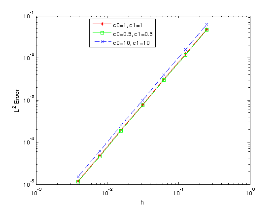 Figure 1
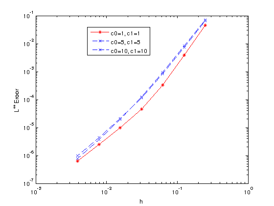 Figure 2
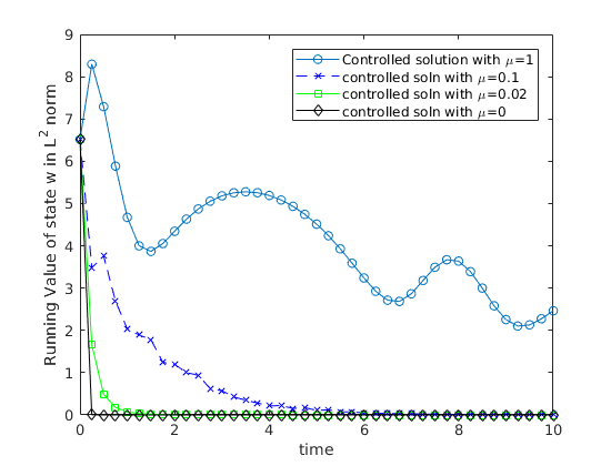 Figure 3
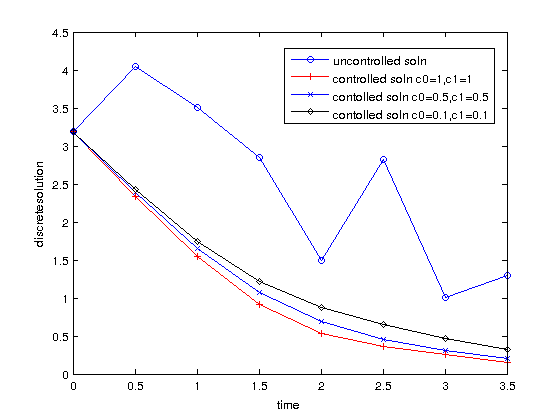 Figure 4
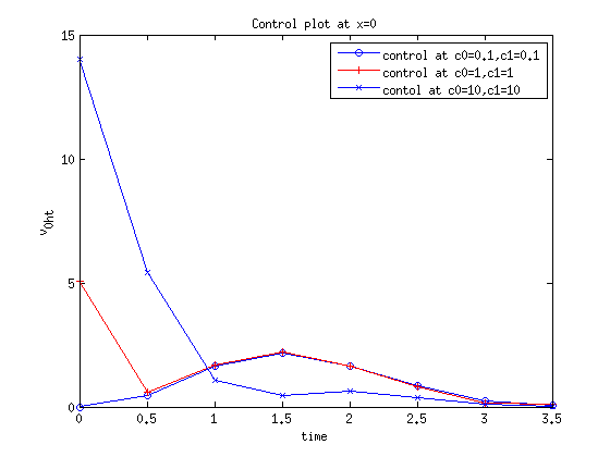 Figure 5
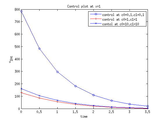 Figure 6
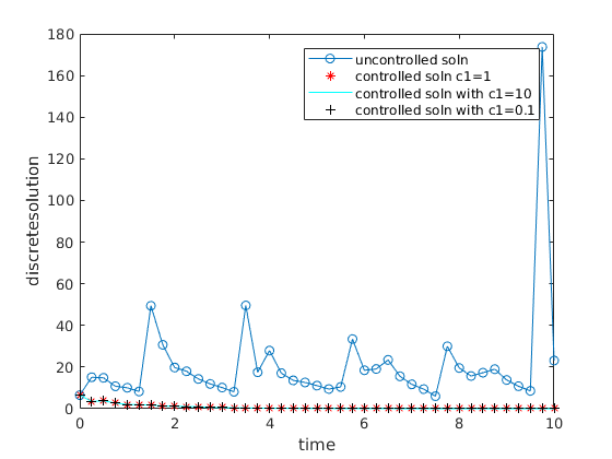 Figure 7
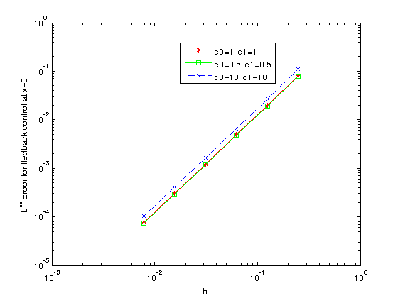 Figure 8
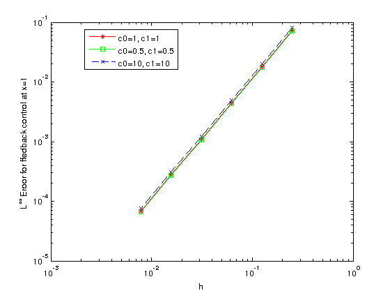 Figure 9
Peer Reviews
No public reviews on file for this paper yet. If you reviewed it on a platform where reviews are public (OpenReview, ICLR, NeurIPS, ICML), you can paste yours below so the community can read it here.
Videos
No videos yet. Explain this paper in a talk, walkthrough, or lecture? Add one.
Global Stabilization of BBM-Burgers’ Type Equations by Nonlinear Boundary Feedback Control Laws: Theory
and Finite Element Error Analysis
Sudeep Kundu111 Institute of Mathematics and Scientific Computing, University of Graz, Heinrichstr. 36, A-8010 Graz, Austria, Email: [email protected] and Amiya Kumar Pani222 Department of Mathematics, IIT Bombay, Powai, Mumbai-400076, India, Email:[email protected]
Abstract
In this article, global stabilization results for the Benjamin-Bona-Mahony-Burgers’ (BBM-B) type equations are obtained using nonlinear Neumann boundary feedback control laws. Based on the -conforming finite element method, global stabilization results for the semidiscrete solution are also discussed. Optimal error estimates in , and -norms for the state variable are derived, which preserve exponential stabilization property. Moreover, for the first time in the literature, superconvergence results for the boundary feedback control laws are established. Finally, several numerical experiments are conducted to confirm our theoretical findings.
Keywords: Benjamin-Bona-Mahony-Burgers’ equation, Neumann boundary feedback control, Stabilization, Finite element method, Optimal error estimates, Numerical experiments
AMS subject classification: 35B37, 65M60, 65M15, 93D15
1 Introduction
Consider the Benjamin-Bona-Mahony-Burgers’ (BBM-B) equations of the following type: seek and which satisfies
[TABLE]
where, the dispersion coefficient and the dissipative coefficient are constants; and are scalar control inputs. The problem (1.1) describes the unidirectional propagation of nonlinear dispersive long waves with dissipative effect. In case, and the equation (1.1) is known as Benjamin-Bona-Mahony (BBM) equation. When and in (1.1), then it is called Burgers’ equation. For mathematical modeling and physical applications of (1.1), see [20], [2], [3] and references, therein.
Based on distributed and Dirichlet boundary control in feedback form through Riccati operator, local stabilization results for the Burgers’ equation with sufficiently small initial data are established in [4], [5]. Moreover, for local stabilization results using Neumann boundary control, we refer to [7], [11] and [12]. It is to be noted that for viscous Burgers’ equation, global existence and uniqueness results with Dirichlet and Neumann boundary conditions are derived for any initial data in in [18]. Subsequently, based on nonlinear Neumann and Dirichlet boundary control laws, global stabilization results for the Burgers’ equation are proved using a suitable application Lyapunov type functional in Krstic [14], Balogh and Krstic [1]. Later on, adaptive (when is unknown) and nonadaptive (when is known) stabilization results for generalized Burgers’ equations are established in [17], [23] and [24] with different types of boundary conditions. For existence of solution to the problem (1.1)-(1.4), when , we refer to [1] and [17].
For stabilization of the BBM-B equation, the authors in [10] have shown global stabilization results corresponding to with zero Dirichlet boundary condition at one end and Neumann boundary control on the other end. Using a reduced order model, distributed feedback control for the BBM-B equation is discussed in [21]. Also, quadratic -spline finite element method followed by linear quadratic regulator theory to design feedback control, is used to stabilize in [22] without any convergence analysis. In [15], we have shown that, under the uniqueness assumption of the steady state solution, the steady state solution of the problem (1.1) with zero Dirichlet boundary condition is exponentially stable.
In this paper, we discuss global stabilization results using nonlinear Neumann feedback control law. Our second objective is to apply -finite element method to the stabilization problem (1.1)-(1.4) using nonlinear Neumann boundary control laws and discuss convergence analysis. Since to the best of our knowledge, there is hardly any discussion in the literature on the rate of convergence, hence, in this paper, an effort has been made to prove optimal order of convergence of the state variable along with superconvergence result for the feedback control laws. The main contributions of this article are summarized as:
- •
Global stabilization for problem (1.1)-(1.4), that is, convergence of the unsteady solution to the problem (1.1) to its constant steady state solution under nonlinear Neumann boundary control laws (1.2)-(1.3) is proved.
- •
Based on the - conforming finite element method, global stabilization results for the semidiscrete solution are discussed and optimal error estimates are established in , , and norms for the state variable. Moreover, superconvergence results are derived for the nonlinear Neumann feedback control laws.
- •
Finally, some numerical experiments are conducted to confirm our theoretical results.
For related issues of finite element analysis of the viscous Burgers’ equation using nonlinear Neumann boundary feedback control law, we refer to our recent article [16]. Compared to [16], special care has been taken to establish global stabilization results in norms as It is further observed that the decay rate for the BBM-B type equation is less than the decay rate for the viscous Burgers’ equation and as the dispersion coefficient approaches zero, the decay rate also converges to the decay rate for the Burgers’ equation. Finite element error analysis holds for fixed .
For the rest of this article, we denote by the standard Sobolev spaces with norm and for , denotes the corresponding norm. The space consists of all strongly measurable functions with norm
[TABLE]
and
[TABLE]
When there is no confusion, is simply denoted by . The equilibrium or steady state solution of (1.1)-(1.3) satisfies
[TABLE]
Note that any constant is a solution of the steady state problem (1.5)-(1.6). Without loss of generality, we assume that .
Set which satisfies
[TABLE]
where, is the state variable and and are feedback control variables. Since for the problem with zero Neumann boundary condition, the steady state constant solution is not asymptotically stable, we plan to achieve stabilization result through boundary feedback law. The present analysis can be easily extended to the problem with one side control law say for example: when , , see [10]. The weak formulation of the problem (1.7)-(1.10) is to seek and such that for almost all
[TABLE]
with For motivation to choose the control laws and using construction of Lyapunov functional, see [14]. Based on the nonlinear Neumann control law propose in our earlier article in Burgers’ equation, see [16], which is a modification of control law in [14], we now choose the feedback control law as
[TABLE]
and
[TABLE]
where and represent feedback control laws, and and are positive constants.
Using (1.12)-(1.13), we obtain a typical nonlinear problem (1.7)-(1.10) with boundary conditions (1.12)-(1.13). Its weak formulation (1.11) becomes
[TABLE]
Throughout the paper, we use the following norm which is equivalent to the usual -norm:
[TABLE]
and is used as a generic positive constant.
We now recall some results to be use in our subsequent sections.
Lemma 1.1**.**
Poincaré-Wirtinger’s inequality* For any , the following inequality holds:*
[TABLE]
Using Agmon’s and Poincaré inequality, the following inequality holds
[TABLE]
where is given in (1.15).
Bellow, we assume the following well posedness theorem for the problem (1.7)-(1.10)
Theorem 1.1**.**
Let Then, there exists a unique weak solution , and of (1.7)-(1.8) satisfying the weak formulation (1.14).
In addition, the following regularity result holds
[TABLE]
Subsequently for our error estimates in norm, we further assumed that with its norm denoted by .
The rest of the article is organized as follows. Section deals with global stabilization results and the existence and uniqueness of strong solution. Section is devoted to optimal error estimates for the semidiscrete solution with superconvergence results for feedback controllers. Finally in section , some numerical examples are considered to confirm our theoretical results.
2 Stabilization and continuous dependence result
In this subsection, we discuss a priori bounds for the problem (1.14) and derive stabilization results. In addition, these estimates are needed to prove optimal error estimates for the state variable and feedback controllers. All estimates throughout the paper are valid for the same with
[TABLE]
Lemma 2.1**.**
Let . Then, there holds
[TABLE]
where is given in (2.1),
[TABLE]
and
[TABLE]
Proof.
Set in the weak formulation (1.14) to obtain
[TABLE]
where is given in (2.3). A use of Young’s inequality for the right hand side term shows
[TABLE]
Therefore, using (2.5) and (2.3), we obtain from (2.4)
[TABLE]
Multiply (2.6) by to arrive at
[TABLE]
A use of Poincaré-Wirtinger’s inequality yields
[TABLE]
Substitute (2.8) in (2.7) and expanding to find that
[TABLE]
Now choose as in (2.1), so that all the coefficients on the left hand side are positive. Then integrating the above inequality from [math] to and multiplying the resulting inequality by we obtain
[TABLE]
This completes the proof. ∎
Remark 2.1**.**
Since
[TABLE]
we obtain from Lemma 2.1
[TABLE]
When Lemma 2.1 holds for all , that is,
[TABLE]
Lemma 2.2**.**
Let . Then, there holds
[TABLE]
where E_{2}(w)(t)=\Big{(}(c_{0}+1+w_{d})+\frac{1}{9c_{0}}w^{2}(0,t)\Big{)}w^{2}(0,t)+\Big{(}(c_{1}+1+w_{d})+\frac{1}{9c_{1}}w^{2}(1,t)\Big{)}w^{2}(1,t).
Proof.
Forming the - inner product between (1.7) and we obtain
[TABLE]
After substituting (1.12)-(1.13) in (2.10), the contributions of the boundary terms in (2.10) are
[TABLE]
The terms on the right hand side of (2.10) are now bounded by
[TABLE]
and
[TABLE]
Using (2.10) we arrive at
[TABLE]
Multiplying the above inequality by and using
[TABLE]
and we obtain
[TABLE]
A use of Gronwall’s inequality now yields
[TABLE]
From Remark 2.1 and Lemma 2.1, we bound the right hand side term of (2.13). Therefore, after multiplying (2.13) by we obtain
[TABLE]
Since the terms in the bracket in the exponential form are bounded, this completes the rest of the proof. ∎
Lemma 2.3**.**
Let . Then, there holds
[TABLE]
where
[TABLE]
Proof.
Set in the weak formulation (1.14) to obtain
[TABLE]
where is given in (2.3). Note that
[TABLE]
and
[TABLE]
Therefore, from (2.15), we arrive at
[TABLE]
Multiply the above inequality by . Now, a use of the Gronwall’s inequality and Lemma 2.1 completes the rest of the proof. ∎
Lemma 2.4**.**
Let . Then, there holds
[TABLE]
where is as in (2.3).
Proof.
Differentiating (1.7) with respect to and then taking the inner product with , we obtain
[TABLE]
The other terms in (2.16) are bounded by
[TABLE]
and
[TABLE]
Therefore, from (2.16), we arrive at
[TABLE]
Now multiply the above inequality by to obtain
[TABLE]
By the Gronwall’s inequality, it follows from above with a use of Lemmas 2.1 and 2.3 that
[TABLE]
Also after putting in the weak formulation (1.14), we arrive at
[TABLE]
Therefore, we can find the value of at as
[TABLE]
Hence, we arrive at
[TABLE]
Multiply the above inequality by to complete the proof. ∎
Lemma 2.5**.**
Let . Then, there holds
[TABLE]
Proof.
Form the -inner product between (1.7) and to obtain
[TABLE]
where we use the bound of and for from Lemma 2.2.
Multiply (2.17) by to obtain
[TABLE]
Integrate from [math] to and then multiply the resulting inequality by with a use of Lemmas 2.2 and 2.4 to arrive at
[TABLE]
This completes the proof. ∎
2.1 Continuous dependence property
Below, we show a continuous dependence property from which uniqueness follows.
Lemma 2.6**.**
For two different initial conditions and the following continuous dependence property holds
[TABLE]
where , and is same as in (2.23).
Proof.
Let and be two solutions of (1.7) with boundary conditions (1.12), (1.13) and initial conditions and , and set . Then, satisfies
[TABLE]
In its weak formulation, seek such that
[TABLE]
Set in (2.22), and bound the fourth and fifth terms on the left hand side, respectively, as
[TABLE]
and
[TABLE]
Now to bound the other terms on the left hand side of (2.22), we rewrite the following terms as for
[TABLE]
and
[TABLE]
Therefore, from (2.22), we arrive at
[TABLE]
Setting
[TABLE]
we obtain
[TABLE]
Applying Gronwall’s inequality to the above inequality yields
[TABLE]
A use of Lemmas 2.2-2.4 gives the desired result. ∎
As a consequence, when it follows that for all . Hence, the solution is unique.
3 Finite element approximation
In this section, we discuss semidiscrete Galerkin approximation keeping the time variable continuous. Moreover, optimal error estimates for the state variable and superconvergence results for feedback controllers are established.
For any positive integer let be a partition of into subintervals with and mesh parameter . We define a finite dimensional subspace of as follows
[TABLE]
where is the set of linear polynomials in .
Now, the corresponding semidiscrete formulation for the problem (3.3)-(3.6) is to seek such that
[TABLE]
with an approximation of . For our analysis, we assume that is the projection of onto .
Now since is finite dimensional, the semidiscrete problem (3.1) leads to a system of nonlinear ODEs. Then an appeal to the Picard’s theorem yields the existence of a unique solution in for some . Since from Lemma 3.1, is bounded for all using a continuation argument, the global existence of is established.
Below, we state four Lemmas for the semidiscrete problem (1.7)-(1.10), which imply global stabilization result for the semidiscrete solution.
Lemma 3.1**.**
Let . With as in (2.1), there holds
[TABLE]
where
[TABLE]
and is the same as in (2.2).
Proof.
For the proof we can proceed as in continuous case. ∎
One dimensional discrete Laplacian is defined by
[TABLE]
The semidiscrete version of the control problem (1.7)-(1.10) satisfies
[TABLE]
where following estimates hold:
[TABLE]
Using (3.7), we can show that and . For showing the bound of we rewrite
[TABLE]
Choose so that from Lemma 3.5, we obtain the bound of and . Now a use of inverse inequality yields easily.
Lemma 3.2**.**
Let . Then, there holds
[TABLE]
where
[TABLE]
Lemma 3.3**.**
Let . Then, there holds
[TABLE]
where
[TABLE]
Lemma 3.4**.**
Let . Then, there holds
[TABLE]
where is as in previous Lemma 3.3.
Remark 3.1**.**
The proofs of the above Lemmas 3.2-3.4 follows in a similar fashion as in continuous case. Also for all results in these lemmas hold.
3.1 Error estimates
To bound the error, we first introduce an auxiliary projection of through the following form
[TABLE]
where is some fixed positive number. For a given the existence of a unique follows from the Lax-Milgram Lemma. Let be the error involved in the auxiliary projection. Then, the following standard error estimates hold
[TABLE]
and
[TABLE]
For a proof, we refer to Thomée [25]. In addition, for proving optimal error estimates, we need the following estimates of and at the boundary points whose proof can be found out in [16] and [19].
Lemma 3.5**.**
For there holds
[TABLE]
Using elliptic projection, write
[TABLE]
Choose so that .
Since estimates of are known, it is enough to estimate . Subtracting (3.1) from (1.14) and using (3.8), we arrive at
[TABLE]
where for can be rewritten as
[TABLE]
Lemma 3.6**.**
Assume that . Then, there exists a positive constant independent of such that
[TABLE]
where \beta_{1}=\min\Bigg{\{}(\frac{3\nu}{2}-2\alpha(\mu+1)),\Big{(}1-2\alpha\big{(}\frac{2\mu}{\nu}+1\big{)}\Big{)}\Bigg{\}}>0.
Proof.
Set in (3.11) to obtain
[TABLE]
where and are last two summation term respectively. The first term on the right hand side of (3.12) is bounded using the Cauchy-Schwarz inequality and the Young’s inequality in
[TABLE]
where constant we choose later. For the second term on the right hand side of (3.12), integration by parts, the Cauchy-Schwarz inequality, and Young’s inequality yield
[TABLE]
For the third term, we note that
[TABLE]
First subterms of the fourth and fifth term on the right hand side of (3.12) are bounded by
[TABLE]
For second subterm of the fourth term on the right hand side, we note that for
[TABLE]
Using Young’s inequality, implies that for
[TABLE]
[TABLE]
and
[TABLE]
Again, a use of Young’s inequality yields
[TABLE]
Hence, the contribution of the second subterm of the fourth term on the right hand side of (3.12) after applying Lemmas 2.2, 2.4 and 3.5, can be bounded as
[TABLE]
Expanding the second subterm of the fifth term, we note that for
[TABLE]
[TABLE]
and using Lemmas 2.2 and 2.4, we obtain
[TABLE]
Also, it holds that
[TABLE]
Rewrite and use the Young’s inequality to obtain
[TABLE]
Similarly,
[TABLE]
Hence, from (3.12), we arrive using Lemmas 2.2, 2.4, 3.2, 3.4 and 3.5 at
[TABLE]
Multiply the above inequality by . Use Poincaré-Wirtinger’s inequality
[TABLE]
with
[TABLE]
This yields
[TABLE]
where . Now integrate from [math] to and choose with
[TABLE]
to find that
[TABLE]
where \psi(t)=\sum_{i=0}^{1}\Big{(}w^{2}(i,t)+w_{t}^{2}(i,t)+w_{h}^{2}(i,t)+\mu w_{ht}^{2}(i,t)\Big{)}. Then, an application of Gronwall’s inequality to (3.14) shows
[TABLE]
Multiplying (3.16) by and using Lemmas 2.2, 2.4, 3.2 and 3.4 with it follows that
[TABLE]
This completes the proof. ∎
Lemma 3.7**.**
Assume that . Then, there exists a positive constant C independent of h such that
[TABLE]
Proof.
Set in (3.11) to obtain
[TABLE]
The first term on the right hand side of (3.17) is bounded by
[TABLE]
For the second term first rewrite it as
[TABLE]
A use of Young’s inequality shows
[TABLE]
For the third term on the right hand side of (3.17), we first rewrite it as
[TABLE]
and then an application of Young’s inequality with Lemmas 2.2, 2.4 and 3.2 yields
[TABLE]
The first subterm of the fourth term on the right hand side of (3.17) can be rewritten for as
[TABLE]
Hence, we obtain
[TABLE]
For second subterm of the fourth term on the right hand side, we note that for
[TABLE]
Using Lemma 2.2, it follows that for
[TABLE]
[TABLE]
and
[TABLE]
Also, we obtain
[TABLE]
We note that
[TABLE]
The first subterm of the fifth term on the right hand side is bounded by
[TABLE]
For the second subterm of the fifth term we note that for
[TABLE]
[TABLE]
Using Lemmas 2.2 and 3.5, it follows that
[TABLE]
Also, it is valid using Young’s inequality that
[TABLE]
[TABLE]
Using Lemma 3.2, it follows that
[TABLE]
Hence, from (3.17), we obtain using Lemmas 2.4 and 3.5
[TABLE]
where
[TABLE]
Multiply the above inequality by and use Lemmas 2.2, 2.3, 3.2 and 3.5 with bounds of nonlinear boundary terms as in Lemma 3.6 to arrive at
[TABLE]
Integrate from [math] to and then multiply the resulting inequality by to obtain
[TABLE]
Use Young’s inequality and Lemma 2.2 to obtain
[TABLE]
Again using Young’s inequality and Lemma 2.2, we arrive at
[TABLE]
Bounding in a similar fashion as in Lemma 3.6, we obtain a bound for the nonlinear boundary terms as follows
[TABLE]
Finally, apply Grönwall’s inequality to (3.18) to arrive using Lemmas 2.2, 2.4, 3.1-3.3 and 3.6 at
[TABLE]
This completes the proof. ∎
Remark 3.2**.**
As a consequence of Lemma 3.7, we obtain superconvergence result for which depends on . However, for proving optimal estimate, only one modification may be made to compute . Hence, we obtain
[TABLE]
which does not depend on . Now using triangle inequality with Lemmas 3.6 and 3.7 and (3.19), we obtain the following result.
Theorem 3.1**.**
Let . Then, the following error estimates hold for the state and control variables
[TABLE]
where and
[TABLE]
Proof.
The proof follows from Lemmas 2.4, 3.6 and 3.7 with a use of triangle inequality and (3.9). ∎
Theorem 3.2**.**
For there exists a constant such that
[TABLE]
and
[TABLE]
where .
Proof.
From Lemma 3.7, we obtain a superconvergence result for . Using the Poincaré-Wirtinger’s inequality, it follows that
[TABLE]
Now a use of triangle inequality with estimates of and we arrive at the estimate (3.21). To find (3.22), we note that the error in the control law is given by
[TABLE]
Similarly, it follows that
[TABLE]
This completes the proof. ∎
4 Numerical experiments
In this section, we discuss the fully discrete finite element formulation of (1.7) using backward Euler method with Neumann boundary control laws. Here, the time variable is discretized by replacing the time derivative by difference quotient. Let be the approximation of in at Let denote the time step size and where is nonnegative integer. For smooth function defined on set and .
Using backward Euler method, the fully discrete scheme corresponding is a solution of
[TABLE]
with At each time level , the nonlinear algebraic system (4.1) is solved by Newton’s method with initial guess . For implicit scheme (4.1) in our case, CFL condition is not needed. We take time step and mesh size .
Example 4.1**.**
Here, we have taken the initial guess (exact solution at ) where is a constant steady solution for the original problem. We do not know the exact solution . Choose . We consider zero Neumann boundary condition, which is without control and mark it as uncontrolled solution. Then to check whether constant steady state solution is asymptotically stable, we take nonlinear Neumann boundary feedback controllers which are given in (1.8)-(1.9) for different values of and with and .
From the line denoted as ’uncontrolled soln’ in Figure 1, we can clearly observe that does not go to zero, that is, constant steady state solution is not asymptotically stable with zero Neumann boundaries. We now observe that for various combination of and , the discrete solution goes to zero exponentially, see Figure 1. Moreover from Figure 1, we can see that the optimal decay rate (with ), 0<\alpha\leq\frac{1}{2}\min\Big{\{}\frac{\nu}{\mu+1},\frac{\nu}{2\mu+\nu},\frac{\nu(4+c_{i})}{\nu+(4+c_{i})\mu}(i=0,1)\Big{\}} happens when , which verify our theoretical result in Lemma 2.1. When , then decay rate for the state is slow compare to the case when .
Now, we present order of convergence for the error in state variable in and norms ( and respectively) and also for the feedback controllers and ( and ) in norm at . Exact solution is obtained through refined mesh solution.
Figures 3 and 3 indicate the error plot for the state variable in and norms respectively, for various values of and . We can easily observe from Figure 3 that the convergence rate in the - norm for error in state variable is of order as predicted by Theorem 3.1. From Figure 3, it is also noticeable that the order of convergence for error in state variable in norm is as expected from Theorem 3.2.
For error in feedback controllers at and it is observed from Figures 5 and 5 that for various values of and the order of convergence is which confirms the result in Theorem 3.2. In Figures 7 and 7, we present the behavior of the feedback controllers at and with respect to time for various positive values of and . Absolute value of the feedback controllers go to zero as time increases. So for in the feedback control law, it will take more time for the control and state to settle down to zero (See Figures 1, 7 and 7).
The next example consists of different type feedback control which is stated below. In the following example, we consider the solution of (1.7) with one part zero Dirichlet boundary and another part different Neumann conditions.
Example 4.2**.**
*In this example, we consider the solution of (1.7) with different boundary conditions. Take initial condition as , where is the steady state solution. We choose time and the time step and and .
For the uncontrolled solution, we take and . The uncontrolled solution is denoted by ’uncontrolled soln’ in Figure 9.
For the controlled solution we consider and w_{x}(1,t)=v_{1}(t)=-\frac{1}{\nu}\Big{(}(c_{1}+1+w_{d})w(1,t)+\frac{2}{9c_{1}}w^{3}(1,t)\Big{)} with and . Denote the controlled solutions by ’controlled solution ’, ’controlled solution with ’, and ’controlled solution with ’ in Figure 9.*
First draw line in Figure 9 shows that solution with zero boundary conditions ( and ) oscillate. But using above mentioned type of control with different values of , solution goes to zero. With the initial condition of Example 4.2, decay of the state in - norm varying with fixed , is shown in Figure 9. We observe that as decreases, - norm of the state for BBM-B equation converges to the - norm of the state with that is to the - norm of the state of Burgers’ equation.
5 Conclusion
In this article, under the assumption of the existence of solution, we show stabilization estimate in higher order norms which is crucial to obtain optimal error estimates in the context of - conforming finite element analysis. Optimal error estimates for the state variable in , and norms are established. Furthermore, superconvergence results for error in feedback controllers are also proved. Following points which are itemized below will be addressed in a separate paper.
- •
When the coefficient of viscosity is unknown (in the case of adaptive control), we believe that the control law as in Smaoui [23] will also work for BBM-B equation. Also when , it is interesting to extend the analysis modifying the control law appropriately.
- •
On the other hand, we have not discussed rigorously the existence of solution of problem (1.7)-(1.10), namely Theorem 1.1.
- •
In addition, for the fully discrete scheme (4.1), it is interesting to know the large time behavior of the solution and how the corresponding time step size behaves in error estimates for fully discrete solution in addition to the space step size .
Acknowledgements. The first author was supported by the ERC advanced grant 668998 (OCLOC) under the EUs H2020 research program. The first author would like to thank Prof. Karl Kunisch for helpful suggestions.
The reference list from the paper itself. Each links out to its DOI / PubMed record.
- 1[1] Balogh, A. and Krstic, M.: Burgers’ equation with nonlinear boundary feedback: H 1 superscript 𝐻 1 H^{1} stability well-posedness and simulation , Math. Problems Engg., 6(2000), 189-200.
- 2[2] Benjamin, T. B. and Bona, J. J. and Mahony, J. J.: Model equations for long Waves in nonlinear dispersive systems , Philos Trans R Soc Lond. A, 272(1972), 47-78.
- 3[3] Bona, J. L.: Model equations for waves in nonlinear dispersive systems , Proceedings of the International Congress of Mathematicians, Helsinki, 1978.
- 4[4] Burns, J. A. and Kang, S.: A control problem for Burgers’ equation with bounded input/output , Nonlinear Dynamics, 2 (1991), 235-262.
- 5[5] Burns, J. A. and Kang, S. : A stabilization problem for Burgers’ equation with unbounded control and observation , Proceedings of an International Conference on Control and Estimation of Distributed Parameter Systems, Vorau, July 8–14, 1990.
- 6[6] Burns, J. A. and Balogh, A. and Gilliam, D. S. and Shubov, V. I.: Numerical Stationary Solutions for a Viscous Burgers’ Equation , Journal of Mathematical Systems, Estimations, and Control, 8(1998), 1-16.
- 7[7] Byrnes, C. I. and Gilliam, D. S. and Shubov, V. I.: On the global dynamics of a controlled viscous Burgers’ equation , J. Dynam. Control Syst., 4(1998), pp. 457-519.
- 8[8] Byrnes, C. I. and Gilliam, D. S. and Shubov, V. I.: Boundary control for a viscous Burgers’ equation , H. T. Banks, R.H. Fabiano, and K. Ito (Eds.), Identification and Control for Systems Governed by Partial Differential Equations, SIAM, 1993, 171-185.