On the Complexity Landscape of Connected f -Factor Problems
R. Ganian, N. S. Narayanaswamy, S. Ordyniak, C. S. Rahul, M. S., Ramanujan

TL;DR
This paper explores the computational complexity of connected f-factor problems in graphs, revealing new thresholds where the problem shifts from polynomial-time solvable to NP-intermediate, depending on the lower bounds of the function f.
Contribution
It extends previous work by establishing new complexity results for connected f-factor problems based on restrictions on the function f.
Findings
Connected f-factor is NP-complete in general.
When f(v) >= n/(log n)^c, the problem is quasi-polynomial or randomized polynomial-time solvable for c<=1.
For c>1, the problem is NP-intermediate.
Abstract
Let G be an undirected simple graph having n vertices and let f be a function defined to be f:V(G) -> {0,..., n-1}. An f-factor of G is a spanning subgraph H such that degree of a vertex v in H is f(v) for every vertex v in V(G). The subgraph H is called a connected f-factor if, in addition, H is connected. A classical result of Tutte(1954) is the polynomial time algorithm to check whether a given graph has a specified f-factor. However, checking for the presence of a connected f-factor is easily seen to generalize HAMILTONIAN CYCLE and hence is NP-complete. In fact, the CONNECTED f-FACTOR problem remains NP-complete even when we restrict f(v) to be at least n^e for each vertex v and 0<e<1; on the other side of the spectrum of nontrivial lower bounds on f, the problem is known to be polynomial time solvable when f(v) is at least n/3 for every vertex v. In this paper, we extend this line…
Click any figure to enlarge with its caption.
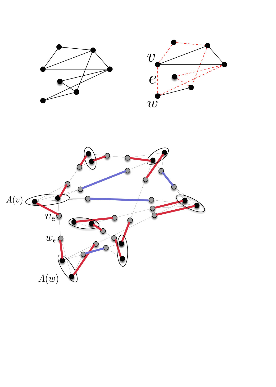 Figure 1
Peer Reviews
No public reviews on file for this paper yet. If you reviewed it on a platform where reviews are public (OpenReview, ICLR, NeurIPS, ICML), you can paste yours below so the community can read it here.
Videos
No videos yet. Explain this paper in a talk, walkthrough, or lecture? Add one.
Taxonomy
TopicsAdvanced Graph Theory Research · Complexity and Algorithms in Graphs · Limits and Structures in Graph Theory
∎
11institutetext: 1Algorithms and Complexity Group, TU Wien, Vienna, Austria
[email protected], [email protected]
2Indian Institute of Technology Madras, Chennai, India
3Department of Computer Science, University of Sheffield, Sheffield, UK
4Faculty of Mathematics, Informatics and Mechanics, University of Warsaw, Poland
On the Complexity Landscape of Connected -Factor Problems
R. Ganian1
N. S. Narayanaswamy2
S. Ordyniak3
C. S. Rahul4
M. S. Ramanujan1
Abstract
Let be an undirected simple graph having vertices and let be a function defined to be . An -factor of is a spanning subgraph such that for every vertex . The subgraph is called a connected -factor if, in addition, is connected. A classical result of Tutte (1954) is the polynomial time algorithm to check whether a given graph has a specified -factor. However, checking for the presence of a connected -factor is easily seen to generalize Hamiltonian Cycle and hence is -complete. In fact, the Connected -Factor problem remains -complete even when we restrict to be at least for each vertex and ; on the other side of the spectrum of nontrivial lower bounds on , the problem is known to be polynomial time solvable when is at least for every vertex .
In this paper, we extend this line of work and obtain new complexity results based on restrictions on the function . In particular, we show that when is restricted to be at least , the problem can be solved in quasi-polynomial time in general and in randomized polynomial time if . Furthermore, we show that when , the problem is -intermediate.
Keywords:
connected -factors, quasi-polynomial time algorithms, randomized algorithms, -intermediate, exponential time hypothesis
1 Introduction
The concept of -factors is fundamental in graph theory, dating back to the 19th century, specifically to the work of Petersen JP1891 . In modern terminology, an -factor is defined as a spanning subgraph which satisfies degree constraints (given in terms of the degree function ) placed on each vertex of the graph DW00 . Some of the most fundamental results on -factors were obtained by Tutte, who gave sufficient and necessary conditions for the existence of -factors WT52 . In addition, he developed a method for reducing the -factor computation problem to the perfect matching WT54 problem, which gives a straightforward polynomial time algorithm for the problem of deciding the existence of an -factor. There are also several detailed surveys on -factors of graphs, for instance by Chung and Graham CG81 , Akiyama and Kano JK85 , Lovász and Plummer LP86 .
Aside from work on general -factors, substantial attention has been devoted to the variant of -factors where we require the subgraph to be connected (see for instance the survey articles by Kouider and Vestergaard KV05 and Plummer PM07 ). Unlike the general -factor problem, deciding the existence of a connected -factor is -complete GJ79 ; CC90 . It is easy to see that the connected -factor problem (Connected -Factor) generalizes Hamiltonian Cycle (set for every vertex ), and even the existence of a deterministic single-exponential (in the number of vertices) algorithm is open for the problem PhilipR14 .
The -completeness of this problem has motivated several authors to study the Connected -Factor for various restrictions on the function . Cornelissen et al. BN13 showed that Connected -Factor remains -complete even when is at least for each vertex and any constant between 0 and 1. Similarly, it has been shown that the problem is polynomial time solvable when is at least NR15 for every vertex . Aside from these two fairly extreme cases, the complexity landscape of Connected -Factor based on lower bounds on the function , has largely been left uncharted.
Our results and techniques. In this paper, we provide new results (both positive and negative) on solving Connected -Factor based on lower bounds on the range of . Since we study the complexity landscape of Connected -Factor through the lens of the function , it will be useful to formally capture bounds on the function via an additional “bounding” function . To this end, we introduce the connected -Bounded -factor problem (Connected -Bounded -Factor) below:
Connected -Bounded -Factor
Instance: An -vertex undirected simple graph and a mapping
such that .
Task: Find a connected -factor of .
First, we obtain a polynomial time algorithm for Connected -Factor when is at least for every vertex and any constant . This result generalizes the previously known polynomial time algorithm for the case when is at least . This is achieved thanks to a novel approach for the problem, which introduces a natural way of converting one -factor to another by exchanging a set of edges. Here we formalize this idea using the notion of Alternating Circuits. These allow us to focus on a simpler version of the problem, where we merely need to ensure connectedness across a coarse partition of the vertex set. Furthermore, we extend this approach to obtain a quasi-polynomial time algorithm for the Connected -Factor when is at least for every vertex. To be precise, we prove the following two theorems (see Section 2 for an explanation of the function in formal statements).
Theorem 1.1
For every function , Connected -Bounded -Factor can be solved in polynomial time.
Theorem 1.2
For every and function , Connected -Bounded -Factor can be solved in time where .
Second, we build upon these new techniques to obtain a randomized polynomial time algorithm which solves Connected -Factor in the more general case where is lower-bounded by for every vertex and . For this, we also require algebraic techniques that have found several applications in the design of fixed-parameter and exact algorithms for similar problems CyganNPPRW11 ; Wahlstrom13 ; GutinWY13 ; PhilipR14 . Precisely, we prove the following theorem.
Theorem 1.3
For every function , Connected -Bounded -Factor can be solved in polynomial time with constant error probability.
We remark that the randomized algorithm in the above theorem has one-sided error with ‘Yes’ answers always being correct. Finally, we obtain a lower bound result for Connected -Factor when is at least for . Specifically, in this case we show that the problem is in fact -intermediate, assuming the Exponential Time Hypothesis RF01 holds. Formally speaking, we prove the following theorem.
Theorem 1.4 ()
For every and for every , Connected -Bounded -Factor is neither in nor -hard unless the Exponential Time Hypothesis fails.
We detail the known as well as new results on the complexity landscape of Connected -Factor in Table 1.
Organization of the paper. After presenting required definitions and preliminaries in Section 2, we proceed to the key technique and framework used for our algorithmic results, which forms the main part of Section 3. In Section 3.2, we obtain both of our deterministic algorithms, which are formally given as Theorem 1.1 (for the polynomial time algorithm) and Theorem 1.2 (for the quasi-polynomial time algorithm). Section 4 then concentrates on our randomized polynomial time algorithm, presented in Theorem 1.3. Finally, Section 5 focuses on ruling out (under established complexity assumptions) both -completeness and inclusion in possibilities for Connected -Bounded -Factor for all polylogarithmic functions in .
2 Preliminaries
2.1 Basic Definitions
We use standard definitions and notations from West DW00 . The notation denotes the degree of a vertex in a graph . Similarly, represents the set of vertices adjacent to in . A component in a graph is a maximal subgraph that is connected. Note that the set of components in a graph uniquely determines a partition of the vertex set. A circuit in a graph is a cyclic sequence where each is of the form and occurs at most once in the sequence. An Eulerian circuit in a graph is a circuit in which each edge in the graph appears. Any graph having an Eulerian circuit is called an Eulerian graph.
Let be a subset of the vertices in the graph . The vertex induced subgraph is the graph over vertex set containing all the edges in whose endpoints are both in . Given , is the edge induced subgraph of whose edge set is and vertex set is the set of all vertices incident on edges in .
Given two subgraphs and of , the graph is the subgraph . The union of the graphs is the graph whose vertex set is and edge set is .
Given a partition of the vertex set of , the quotient graph is constructed as follows: The vertex set of is . Corresponding to each edge in where in , in , , add an edge to . Thus, is a multigraph without loops. For a subgraph of , we say connects a partition if is connected. Further, we address the graph to be a partition connector. A refinement of a partition is a partition of where each part in is a subset of some part in . This notion of partition refinement was used, e.g., by Kaiser TK12 . A spanning tree of the quotient graph refers to a subgraph of with -1 edges that connects . The following lemma will later be used in the analysis of the error probability of our randomized algorithm.
Lemma 1
The following holds for every with :**
[TABLE]
Proof
Using simple term manipulations, we obtain:
[TABLE]
Since , it follows that:
[TABLE]
By using the binomial formula, we obtain:
[TABLE]
To obtain an upper bound on , we show next that the absolute values of the terms in the sum are decreasing with increasing .
[TABLE]
The first inequality above holds because . Hence, we obtain.
[TABLE]
Putting the above back into Equation 1 and using Inequality 2 together with the expressions above, we obtain:
[TABLE]
The above concludes the proof of the lemma. ∎
The function we deal with is always a positive real-valued function, defined on the set of positive integers. For the cases we consider, the function always takes a value greater than 1. Unless otherwise mentioned, is in . Whenever is part of the problem definition, the target set of the function is the set of integers . Consequently, we have the following fact.
Fact 2.1
Let be a graph and let for each in . If is an -factor of , then the number of components in is at most .
2.2 Colored Graphs, (Minimal) Alternating Circuits, and -Factors
A graph is colored if each edge in is assigned a color from the set . In a colored graph , we use and to denote spanning subgraphs of whose edge sets are the set of red edges () and blue edges () respectively. We use this coloring in our algorithm to distinguish between edge sets of two distinct -factors of the same graph . A crucial computational step in our algorithms is to consider the symmetric difference between edge sets of two distinct -factors and perform a sequence of edge exchanges preserving the degree of each vertex. The following definition is used extensively in our algorithms.
Definition 1
A colored graph is an alternating circuit if there exists an Eulerian circuit in , where each pair of consecutive edges are of different colors.
Clearly, an alternating circuit has an even number of edges and is connected. Further, for each in . A minimal alternating circuit is an alternating circuit where each vertex in has at most two red edges incident to . Note that alternating circuits, as opposed to Eulerian circuits, cannot always be decomposed into edge-disjoint alternating circuits that are cycles. As an example, consider for each the alternating circuit which consists of two (edge-disjoint) cycles of length and length , respectively, that share one common vertex . Let the coloring of the edges of be as illustrated in Figure 1. Informally, the edges of both cycles are colored in an alternating manner along each cycle so that the edges of the first cycle incident to have the same color, which is distinct from the color given to the edges incident with in the second cycle. Every alternating circuit in contains all edges of and cannot be decomposed further into smaller alternating circuits.
Fact 2.2
Let be a subset of . An -factor of containing all the edges in , if one exists, can be computed in polynomial time.
The fact follows from the observation that a candidate for can be computed from an -factor of the spanning subgraph , where for each . Note that given a partition of , one can check for the existence of an -factor connecting in polynomial time by iterating over each edge in the cut and applying Fact 2.2 by setting . Further, this can be extended for any arbitrary partition of constant size, or when we are provided with a spanning tree of that is guaranteed to contain in some -factor of .
Definition 2
Let and be two subgraphs of where each component in is Eulerian. Let be the unique coloring function which colors the edges in with color red and those in with color blue. The subgraph is called a switch on if every component of the colored graph obtained by applying c on , is an alternating circuit.
Definition 3
For a subgraph which is a switch on another subgraph of , we define Switching(,) to be the subgraph of .
We use switching as an operator where the role of the second operand is to bring in specific edges to the first, retaining the degrees of vertices by omitting some less significant edges. One can easily infer that if the result of applying the coloring function c to is a minimal alternating circuit, then the switching operation replaces at most two edges incident on each vertex in .
Fact 2.3
Let be an alternating circuit and be a subset of edges in . There is a polynomial time algorithm that outputs a set of edge disjoint minimal alternating circuits in , each of which has at least one edge from and such that every edge in is contained in some minimal alternating circuit in .
It is not difficult to see the proof of Fact 2.3. A skeptical reader can refer (NR15, , Lemma 6). Note that given and , is not unique.
Fact 2.4
Let be an -factor of and let be a partitioning of the vertex set of . If is connected and is connected for each in , then is a connected -factor.
Fact 2.4 implies that if is not a connected -factor and is connected then there exists some such that is not connected.
3 A Generic Algorithm for Finding Connected -Bounded -Factors
Our goal in this section is to present a generic algorithm for Connected -Bounded -Factor. In particular, we in a certain sense reduce the question of solving Connected -Bounded -Factor to solving a related problem which we call Partition Connector. This can be viewed as a relaxed version of the original problem, since instead of a connected -factor it merely asks for an -factor which connects a specified partitioning of the vertex set. A formal definition is provided below.
Partition Connector
Instance: An -vertex graph , , and a partition of .
Task: Find an -factor of that connects .
The algorithms for solving Partition Connector are presented in the later parts of this article. Specifically, a deterministic algorithm that runs in quasi-polynomial time whenever (Section 3.2) and a randomized polynomial time algorithm for the case when (Section 4).
The majority of this section is devoted to proving the key Theorem 3.1 stated below, which establishes the link between Partition Connector and Connected -Bounded -Factor.
Theorem 3.1
Let . If there is a deterministic algorithm running in time 111We use to denote , i.e., omits polynomial factors, for any function . for Partition Connector, then there is a deterministic quasi-polynomial time algorithm for Connected -Bounded -factor with running time .
*Let . If there exists a randomized algorithm running in time with error probability for Partition Connector, then there exists a randomized polynomial time algorithm for Connected -Bounded -factor that has a constant error probability. *
3.1 A generic algorithm for Connected -Bounded -Factor
The starting point of our generic algorithm is the following observation.
Observation 3.2
Let be an undirected graph and be a function . The graph has a connected -factor if and only if for each partition of the vertex set , there exists an -factor of that connects .
We remark that for the running time analysis for our generic algorithm we assume that we are only dealing with instances of Connected -Bounded -Factor, where the number of vertices exceeds . As is in , this does not reduce the applicability of our algorithms, since there is a constant such that for every ; because is part of the problem description, does not depend on the input instance. Consequently, we can solve instances of Connected -Bounded -Factor where by brute-force in constant time. We will therefore assume without loss of generality in the following that and hence .
Our algorithm constructs a sequence of pairs which is maximal (cannot be extended further) satisfying the following properties:
- (M1)
Each is a partition of the vertex set , and . 2. (M2)
Each is an -factor of , and connects . 3. (M3)
For each , is a refinement of satisfying the following:
- a)
Each part in induces a component in , for some in . 2. b)
.
The following lemma links the existence of a connected -factor to the properties of maximal sequences satisfying (M1)–(M3).
Lemma 2
Let be an instance of Connected -Bounded -Factor and let be a maximal sequence satisfying (M1)–(M3). Then, has a connected -factor if and only if is a connected -factor of .
Proof
Towards showing the forward direction of the claim, suppose for a contradiction that is not a connected -factor of . Because connects (Property (M2)), it follows from Fact 2.4 that there is some part such that is not connected. Consider the refinement of () that splits every part in into the parts corresponding to the components of . Further, because has a connected -factor and Observation 3.2, we obtain that there exists a connected -factor that connects any partition . Now, the sequence could be extended by appending the pair to its end, a contradiction to our assumption that was a maximal sequence. The reverse direction is trivial. ∎
We deploy an algorithm that incrementally computes a maximal sequence satisfying (M1)–(M3) and thereby use the above lemma to solve the connected -factor problem by testing whether the last -factor in the sequence is connected. This involves computing from and followed by the computation of connecting . However, if the number of parts in the last partition is allowed to grow to , then such an algorithm would eventually have to solve the connected -factor problem to compute an satisfying (M2). Our algorithm establishes a lower bound on the size of any part and hence an upper bound on the number of parts in any partition in which in turn bounds the length of the sequence .
The following lemma shows that given the recently computed pair in the sequence, the partition and a candidate for , one can compute a better candidate for which is closer to in the sense that most of the neighbors of a vertex in are retained as it is, in . The properties of then allow us to lower-bound the size of each part in as a function of the size of the smallest part in .
Lemma 3
Let , be two consecutive pairs occurring in a sequence satisfying properties (M1)–(M3). Then, there is an -factor of connecting such that for every and . Moreover, can be computed from , , and in polynomial time.
Proof
From the premise that is an -factor connecting , we know that there exists a spanning tree of . Color the edges in with color red and those in with color blue. Let be the graph . Notice that each component in is an alternating circuit. Furthermore, note that the set of blue edges is a subset of as is a subset of . Let be the set where is the component in . We compute the set of edge disjoint minimal alternating circuits using Fact 2.3 for each pair. The size of the set is at most and hence at most minimal alternating circuits in . Let and be the -factor defined as Switching(,). We argue that this switching operation removes at most edges incident on any vertex in for every .
Considering the fact that the minimal alternating circuits in are edge disjoint, we visualize switching with as a sequence of switching operations on each with a distinct minimal alternating circuit in . In each such , the number of red edges incident on a vertex that leaves during switching is at most two and the operation Switching(,) retains at least neighbors of each vertex. Thus, for any subset of if we consider the subgraph alone, it must be the case that for each in . Furthermore, is at most . Since the set is a subset of , connects . From Fact 2.3, the computation of and hence of takes polynomial time. This completes the proof of the lemma. ∎
By employing the above lemma, our algorithm ensures that the maximal sequence so constructed satisfies the following additional property:
- (M4)
For every , every and it holds that .
This property plays a key role in the analysis of our algorithm as it allows us to bound the number of parts in each partition . Towards this aim we require the following auxiliary lemma.
Lemma 4
Let be a sequence satisfying properties (M1)–(M4). Then, for every with , and .
Proof
We show the claim by induction on starting from . Let and . Because is an -factor of and is a component of , we obtain that . Using Property (M4) for , we obtain , as required. Hence assume that the claim holds for and we want to show the claim for . Let and and let be the part in containing . Note that . From the induction hypothesis we obtain that . Because is a component of , it holds that . Hence together with Property (M4), we obtain
[TABLE]
as required. This completes the proof of the lemma. ∎
Recall that is at least for each . Our next step is to show that the length of the maximal sequence constructed by our algorithm does not exceed .
Lemma 5
Let be a maximal sequence satisfying properties (M1)–(M4). Then, for every with . Moreover, the length of is at most .
Proof
The claim clearly holds for . It also holds for because the parts in correspond to the components of , which are at most due to Fact 2.1. Assume for a contradiction that the claim does not hold and let be a maximal sequence satisfying (M1)–(M4) witnessing this and let be the smallest integer such that . Then, and . Because and for every , is larger than , we obtain that for every . Hence, or in other words .
From Lemma 4, we obtain that
[TABLE]
for every and . This implies that every component of for some , and hence also every part of has size at least . Since , we conclude that the number of vertices of is greater than . Rearranging for we obtain that which contradicts our assumption that . Since is a proper refinement of for every with and , we infer that the length of the sequence is at most . This completes the proof of the lemma. ∎
We are now ready to prove the main theorem of this section which outlines how the running time of Connected -Bounded -Factor is dominated by the Partition Connector module.
Proof (Theorem 3.1)
We present an algorithm for Connected -Bounded -factor that employs an algorithm for Partition Connector as a subroutine. All parts of the algorithm apart from the subroutine Partition Connector will be deterministic and run in polynomial time. The main idea is to construct a maximal sequence satisfying properties (M1)–(M4). Recall our assumption that . Let be an instance of Connected -Bounded -factor. The algorithm starts by computing an arbitrary -factor . If no -factor exists, then clearly the algorithm reports failure. If on the other hand the computed -factor is already connected, then the algorithm returns and exits.
Observe that , where , is a valid starting pair for a sequence satisfying properties (M1)–(M4). Further, the algorithm extends the sequence by adding successors as long as one exists. The sequence is extended by invoking a recursive subroutine Restricted--factor with parameters and the most recently added pair to compute a new pair that can be appended to the sequence, if one exists. Otherwise, the procedure concludes that can no longer be extended, in which case it either returns a connected -factor of or reports nonexistence of one. The subroutine Restricted--factor works as follows.
The procedure starts by computing a refinement of containing one part for every component in where is a part in . If then because of Fact 2.4, already constitutes a connected -factor of and the procedure correctly returns . Otherwise, the procedure calls the provided algorithm for Partition Connector on , , and to obtain an -factor connecting . If the provided algorithm for Partition Connector returns failure, the procedure also returns failure, relying on Observation 3.2 and assuming that no -factor connecting exits. Otherwise, observe that the pair already constitutes a valid successor of the pair in any sequence satisfying properties (M1)–(M3). To ensure Property (M4), the procedure now calls a polynomial time subroutine on the pairs and to obtain the desired -factor connecting and such that the pairs and satisfy Property (M4). The existence of such a polynomial time subroutine is from Lemma 3. The procedure now calls itself on the pair . This completes the description of the algorithm.
Note that given the correctness of the algorithm for Partition Connector the correctness of the algorithm follows from Lemma 2. Let us now analysis the running time of the algorithm. Apart from the calls to the provided subroutine for Partition Connector, all parts of the algorithm run in polynomial time. Because the algorithm calls the provided algorithm for Partition Connector at most once for every pair in a maximal sequence satisfying properties (M1)–(M4), we obtain from Lemma 5 that the number of those calls is bounded by . Moreover, from the same lemma, we obtain that the size of a partition given as an input to the algorithm for Partition Connector is at most . Hence, if Partition Connector can be solved in time , then the algorithm runs in time showing the first statement of the theorem. Similarly, if Partition Connector can be solved in time , then the algorithm runs in time , which given shows that the algorithm claimed in the second statement of the theorem runs in polynomial time. We use the following lemma to prove the second part of the theorem.
Lemma 6
The Partition Connector can be solved by a randomized algorithm with running time and error probability .
It remains to show that the randomized algorithm has the stated error probability. Towards this aim we calculate a lower bound on the success probability of the algorithm, i.e., the probability that the algorithm returns a connected -factor of if such an -factor exists. Hence, let us suppose that has a connected -factor. It follows from Observation 3.2 that contains an -factor connecting for every partition of its vertex set. Hence every call to the subroutine Partition Connector is made for a “Yes”-instance, which together with Lemma 6 implies that every such call succeeds with probability at least . Because , we obtain from Lemma 1 that this probability is at least for some constant . Since there are at most such calls, the probability that the algorithm succeeds for all of these calls is hence at least , as required. This completes the proof of the theorem. ∎
3.2 A Quasi-polynomial Time Algorithm for Polylogarithmic Bounds
In this section, we prove Theorem 1.1 and Theorem 1.2. In fact, we prove a more general result, from which both theorems directly follow.
Theorem 3.3 ()
For every and function , the Connected -Bounded -factor problem can be solved in time.
We make use of the following simple lemma.
Lemma 7
Let be a graph having a connected -factor. Let be a partition of the vertex set . There exists a spanning tree of such that for some -factor of , . Furthermore, can be computed from in polynomial time.
Proof
Let be a connected -factor of . For any partition of the vertex set, it follows from Observation 3.2 that is connected. Consider a spanning tree of . Clearly, there exists at least one -factor containing and hence is connected. Once we have , can be computed in polynomial time using Fact 2.2. ∎
In light of Theorem 3.1, it now suffices to prove the following Lemma 8, from which Theorem 3.3 immediately follows.
Lemma 8
Partition Connector* can be solved in time .*
Proof
It follows from Lemma 7 that we can solve Partition Connector by going over all spanning trees of and checking for each of them whether there is an -factor of containing the edges of . The lemma now follows because the number of spanning trees of is at most , which is upper bounded by , and for every such tree we can check the existence of an -factor containing in polynomial time. ∎
4 A Randomized Polynomial Time Algorithm for Logarithmic Bounds
In this section we prove Theorem 1.3. Due to Theorem 3.1, it is sufficient for us to provide a randomized algorithm for Partition Connector with running time and error probability . This is precisely what we do in the rest of this section (Lemma 6). As a first step, we design an algorithm for the “existential version” of the problem which we call -Partition Connector and define as follows.
-Partition Connector
Input: A graph with vertices, , and a partition of .
Question: Is there an -factor of that connects ?
We then describe how to use our algorithm for this problem as a subroutine in our algorithm to solve Partition Connector.
4.1 Solving -Partition Connector in Randomized Polynomial Time
The objective of this subsection is to prove the following lemma which implies a randomized polynomial time algorithm for -Partition Connector when .
Lemma 9
There exists an algorithm that, given the graph , a function , and a partition of , runs in time and outputs
- •
NO* if has no -factor connecting *
- •
YES* with probability at least otherwise.*
We design this algorithm by starting from the exact-exponential algorithm in PhilipR14 and making appropriate modifications. During the description, we point out the main differences between our algorithm and that in PhilipR14 . We now proceed to the details of the algorithm. We begin by recalling a few important definitions and known results on -factors. These are mostly standard and are also present in PhilipR14 , but since they are required in the description and proof of correctness of our algorithm, we state them here.
Definition 4 (-Blowup)
Let be a graph and let be such that for each . Let be the graph constructed as follows:
For each vertex of , we add a vertex set of size to . 2. 2.
For each edge of we add to vertices and and edges for every and for every . Finally, we add the edge .
This completes the construction. The graph is called the -blowup of graph . We use to denote the -blowup of . We omit the subscript when there is no scope for ambiguity.
Definition 5 (Induced -blowup)
For a subset , we define the -blowup of induced by as follows. Let the -blowup of be . Begin with the graph and for every edge such that and , delete the vertices and from . Let the graph be the union of those connected components of the resulting graph which contain the vertex sets for vertices . Then, the graph is called the -blowup of induced by the set and is denoted by .
We now recall the relation between perfect matchings in the -blowup and -factors (see Figure 2).
Lemma 10 (WT54 )
A graph has an -factor if and only if the -blowup of has a perfect matching.
The relationship between the Tutte matrix and perfect matchings is well-known and this has already been exploited in the design of fixed-parameter and exact algorithms Wahlstrom13 ; GutinWY13 ; PhilipR14 .
Definition 6 (Tutte matrix)
The Tutte matrix of a graph with vertices is an skew-symmetric matrix over the set of indeterminates whose element is defined to be
[TABLE]
We use to denote the Tutte matrix of the graph .
Following terminology in PhilipR14 , when we refer to expanded forms of succinct representations (such as summations and determinants) of polynomials, we use the term naive expansion (or summation) to denote that expanded form of the polynomial which is obtained by merely writing out the operations indicated by the succinct representation. We use the term simplified expansion to denote the expanded form of the polynomial which results after we apply all possible simplifications (such as cancellations) to a naive expansion. We call a monomial which has a non-zero coefficient in a simplified expansion of a polynomial , a surviving monomial of in the simplified expansion. Let denote the determinant of the Tutte matrix of the graph .
Proposition 1 (WT47 )
* is identically zero when expanded and simplified over a field of characteristic two if and only if the graph does not have a perfect matching.*
The following basic facts about the Tutte matrix of a graph are well-known. When evaluated over any field of characteristic two, the determinant and the permanent of the matrix (indeed, of any matrix) coincide. That is,
[TABLE]
where is the set of all permutations of . Furthermore, there is a one-to-one correspondence between the set of all perfect matchings of the graph and the surviving monomials in the above expression for when its simplified expansion is computed over any field of characteristic two. We formally state and give a proof of the latter fact for the sake of completeness and because we intend to use this particular formulation of it.
Lemma 11
Let and be as defined above. Then the following statements hold.
If is a perfect matching of a graph , then the product appears exactly once in the naive expansion and hence as a surviving monomial in the sum on the right-hand side of Equation 3 when this sum is expanded and simplified over any field of characteristic two. 2. 2.
Conversely, each surviving monomial in a simplified expansion of this sum over a field of characteristic two must be of the form where is a perfect matching of .
Proof
For the first statement, consider the permutation comprising precisely the 2-cycles . The corresponding monomial given by the definition of over a field of characteristic two is precisely . For every other permutation , the corresponding monomial given by the definition of contains at least one variable where is not mapped to in . This implies that no other monomial in the naive expansion of Equation 3 is equal to even when considered over a field of characteristic two. This completes the argument for the first statement.
We now consider the second statement. First of all, since we only consider simple graphs, we have that for any permutation with a fixed point, the corresponding monomial is 0 since for every . Let denote the set of all permutations in with a cycle of length at least 3. We now argue that for any permutation , the corresponding monomial vanishes in the simplified expansion of Equation 3. In order to do so, we give a bijection such that (a) for every , , (b) for every , , and (c) for every , the monomials corresponding to and are equal over any field of characteristic two.
We first define for a as follows. Note that we have already fixed an ordering of the vertices of . Let be the first vertex of in this ordering which appears in a cycle of length at least 3 in and let denote this cycle. We now define to be the permutation obtained from by inverting and leaving every other cycle unchanged. Finally, for every , simply set .
It is straightforward to see that the resulting mapping is indeed a bijection and moreover, for every as required. Finally, it follows from the definition of that over a field of characteristic two, the factor of the monomial corresponding to contributed by any cycle is the same as that contributed by the inverse of this cycle to the monomial corresponding to . Hence we have the third property and conclude that for any permutation , the corresponding monomial vanishes in the simplified expansion of Equation 3. This implies that the only surviving monomials are those corresponding to permutations in without a fixed point, implying that these permutations comprise only 2-cycles. This in turn implies that any such surviving monomial must correspond to a perfect matching of as required. This completes the proof of the lemma. ∎
Lemma 12 (Schwartz-Zippel Lemma, Schwartz80 ; Zippel79 )
Let be a multivariate polynomial of degree at most over a field such that is not identically zero. Furthermore, let be chosen uniformly at random from . Then,
[TABLE]
Definition 7
For a partition of , and a subset , we denote by the set . Furthermore, with every set , we associate a specific monomial which is defined to be the product of the terms where and , crosses the cut and are as in Definition 4 of the -blowup of . For , we define .
From now on, for a set , we denote by the set . Also, since we always deal with a fixed graph and function , for the sake of notational convenience, we refer to the graph simply as . We now define a polynomial over the indeterminates from the Tutte matrix of the -blowup of , as follows:
[TABLE]
where if a graph has no vertices or edges then we set . In what follows, we always deal with a fixed partition of .
Remark 1
The definition of the polynomial is the main difference between our algorithm and the algorithm in PhilipR14 . The rest of the details are identical. The main algorithmic consequence of this difference is the time it takes to evaluate this polynomial at a given set of points. This is captured in the following lemma whose proof follows from the fact that determinant computation is a polynomial time solvable problem.
Lemma 13
Given values for the variables in matrix , the polynomial can be evaluated over a field of character 2 and size in time .
Proof
The algorithm to evaluate over the field proceeds as follows. Given the values for the variables in the matrix , we go over all and for each , we evaluate and in polynomial time via standard polynomial time determinant computation. Once this value is computed, we multiply their product with the evaluation of the monomial . Since we go over possible sets and for each the computation takes polynomial time, the claimed running time follows. ∎
Having shown that this polynomial can be efficiently evaluated, we will now turn to the way we use it in our algorithm. Our algorithm for -Partition Connector takes as input , evaluates the polynomial at points chosen independently and uniformly at random from a field of size and characteristic 2 and returns Yes if and only if the polynomial does not vanish at the chosen points. In what follows we will prove certain properties of this polynomial which will be used in the formal proof of correctness of this algorithm. We need another definition before we can state the main lemma capturing the properties of the polynomial. Recall that for every , the set is the set of ‘copies’ of in the -blowup of . Furthermore, for a set , we say that an edge crosses the cut if has exactly one endpoint in .
Definition 8
We say that an -factor of contributes a monomial to the naive expansion of the right-hand side of Equation 4 if and only if the following conditions hold.
For every , there is a , and such that and . 2. 2.
For every , there is a such that . 3. 3.
For every , if and for some , then . 4. 4.
For every , if for some , then . 5. 5.
For every such that has no edge crossing the cut , there is a pair of monomials and such that is a surviving monomial in the simplified expansion of , is a surviving monomial in the simplified expansion of , and .
Having set up the required notation, we now state the main lemma which allows us to show that monomials contributed by -factors that do not connect , do not survive in the simplified expansion of the right hand side of Equation 4.
Lemma 14
Every monomial in the polynomial which is a surviving monomial in the simplified expansion of the right-hand side of Equation 4 is contributed by an -factor of to the naive expansion of the right-hand size of Equation 4. Furthermore, for any -factor of , say , the following statements hold.
If does not connect then every monomial contributed by occurs an even number of times in the polynomial in the naive expansion of the right-hand side of Equation 4. 2. 2.
If connects , then every monomial contributed by occurs exactly once in the polynomial in the naive expansion of the right-hand side of Equation 4.
Proof
For the first statement, let be a monomial which survives in the simplified expansion of the right-hand side of Equation 4. Then it must be of the form and must correspond to a perfect matching of . This is a direct consequence of Lemma 11 (2). Let be this perfect matching. We now define an -factor based on and argue that indeed contributes this monomial to the naive expansion of the right-hand size of Equation 4 as per Definition 8. The -factor is defined as follows. An edge is in if and only if the edge . We now argue that contributes .
Consider the first condition in Definition 8. Since , it must be the case that . Since is a perfect matching and the vertices and each have exactly one neighbor other than each other, it must be the case that contains edges and where for some and for some . The fact that the second condition is satisfied follows directly from the definition of . For the third condition, suppose that for some , and , it holds that and . The fact that corresponds to implies that the edges and are in , which in turn implies that the edge is not in . Hence, by definition of , we conclude that . An analogous argument implies that the fourth condition is satisfied as well. We now come to the final condition. Suppose that such that has no edge crossing the cut . Now, observe that for every which crosses the cut the edge , which by definition implies that . We define to be the subset of edges which cross the cut . Hence, for every edge in , the vertices and lie on the same side of the cut . We now define a partition of as follows. For and , an edge is in if and only if . Clearly, is now a partition of . Furthermore, it is easy to see that is a perfect matching of , is a perfect matching of .
Due to Proposition 1, we know that corresponds to a surviving monomial in the simplified expansion of and corresponds to a surviving monomial in the simplified expansion of . Finally, let denote the monomial . It is easy to see that . Furthermore, . Hence we conclude that is indeed contributed by and proceed to the remaining two statements of the lemma. However, before we prove the remaining statements, we need the following claim.
Claim
Let .
If there is no edge of crossing the cut , then each monomial contributed by to the naive expansion of the polynomial is contributed exactly once. 2. 2.
If there is an edge of crossing the cut then does not contribute a monomial to the naive expansion of the polynomial .
Proof
We begin with the proof of the first statement. By Definition 8 it holds that every monomial contributed by contains . Let be the subgraph of induced on and let be the subgraph of induced on . Observe that is an -factor of and is an -factor of . By Proposition 1 and Lemma 10, we know that every -factor of () appears exactly once in the naive expansion of () (since it is nothing but a perfect matching of the -blowup induced by or ).
Therefore, each monomial corresponding to a perfect matching of which is equivalent to appears exactly once in the naive expansion of the polynomial ; similarly, each monomial corresponding to a perfect matching of which is equivalent to appears exactly once in the naive expansion of . Since every monomial contributed by to the naive expansion of is a product of and a monomial each from and , and these monomials themselves occur exactly once in the naive expansion of and respectively, the first statement follows.
We now prove the second statement of the claim. Here, there must be vertices such that , and . Therefore, by Definition 8, we have that no monomial contributed by has the term where . However, contains the term by definition. Therefore, does not contribute a monomial to . This completes the proof of the claim. ∎
Let be the number of connected components of the graph . If is an -factor of that does not connect it must be the case that . Due to the above claim, observe that there are exactly sets such that contributes each of its monomials exactly once to the simplified expansion of the right hand side of Equation 4 and does not contributes any monomials to any other sets . Since is even for , we conclude that Statement 1 holds.
We now move on to Statement 2. That is, we assume that is an -factor that connects . Due to the above claim, we know that does not contribute a monomial to any polynomial where is such that has an edge which crosses the cut . However, since connects , it crosses every cut where . But observe that since is an -factor of it will contribute a monomial to the polynomial when . Hence, we conclude that any monomial contributed by occurs exactly once in the naive expansion of the right-hand side of Equation 4, completing the proof of the lemma. ∎
This implies the following result, which is the last ingredient we need to prove Lemma 9.
Lemma 15
The polynomial is not identically zero over if and only if has an -factor connecting .
Proof (Lemma 9)
It follows from the definition of that its degree is since the number of vertices in the -blowup of is . As mentioned earlier, our algorithm for -Partition Connector takes as input , evaluates the polynomial at points chosen independently and uniformly at random from a field of size and characteristic 2 and returns Yes if and only if the polynomial does not vanish at the chosen points. Due to Lemma 15, we know that the polynomial is identically zero if and only if has an -factor containing and by the Schwartz-Zippel Lemma, the probability that the polynomial is not identically zero and still vanishes upon evaluation is at most . This completes the proof of the lemma. ∎
Having obtained the algorithm for -Partition Connector, we now return to the algorithm for the computational version, Partition Connector.
4.2 Solving Partition Connector in Randomized Polynomial Time
Proof (Lemma 6)
Consider the following algorithm . Algorithm takes as input an -vertex instance of Partition Connector with the partition , along with a separate set of edges that have been previously selected to be included in the partition connector. Let be initialized as . As its first step, Algorithm checks if ; if this is the case, then it computes an arbitrary -factor , and outputs . To proceed, let us denote the algorithm of Lemma 9 as . If , then first calls and outputs NO if outputs NO. Otherwise, it fixes an arbitrary ordering of the edge set and recursively proceeds as follows.
constructs the set of all edges with precisely one endpoint in , and loops over all edges in (in the ordering given by ). For each processed edge between and some (), it will compute a subinstance defined by setting:
- •
, and
- •
, and for all the remaining vertices of , and
- •
is obtained from by merging and into a new set; formally (assuming , .
Intuitively, each such new instance corresponds to forcing the -factor to choose the edge . then queries on . If answers NO for each such tuple obtained from each edge in , then immediately terminates and answers NO. Otherwise, let be the first edge where answered YES; then adds into . If then the algorithm computes an arbitrary -factor of and outputs . On the other hand, if then restarts the recursive procedure with ; observe that .
Before arguing correctness, we show that the algorithm runs in the required time. Since each edge in the partitioning is processed at most times, the runtime of is asymptotically upper-bounded by its at most many calls to . From Lemma 9, we then conclude that the total runtime of is upper-bounded by .
For correctness, let us first consider the hypothetical situation where always answers correctly. If no partition connector exists, then correctly outputs NO after the first call to . Otherwise, there exists a partition connector, and such a partition connector must contain at least one edge in at every recursion of the algorithm. This implies that would output YES for at least one edge of . Moreover, it is easily seen that for any partition connector containing , is also a partition connector in , and so by the same argument would also output YES for at least one edge in the individual sets constructed in the recursive calls of . In particular, if would always answer correctly, then would correctly output a partition connector at the end of its run. For further considerations, let us fix the set which would be computed by under the assumption that always answers correctly; in other words, is the lexicographically first tuple of edges in which intersects a partition connector.
We are now ready to argue that succeeds with the desired probability; recall that only allows one-sided errors. So, if the input is a no-instance, then is guaranteed to correctly output NO after the first query to . Furthermore, by the definition of , for each edge processed by , the algorithm must also answer NO on . So, assuming always answers correctly, in total would only be called at most times on yes-instances, and in all remaining calls it receives a no-instance. Given that has a success probability of at least , the probability that is called at most times on YES-instances (not counting the initial call on ), and that it succeeds in all these calls, is at least . Hence the error probability of the algorithm is at most . This completes the proof of the lemma. ∎
5 Classification Results
In this section, we prove Theorem 1.4 which we restate for the sake of completeness.
See 1.4
The result relies on the established Exponential Time Hypothesis, which we recall below.
Definition 9 (Exponential Time Hypothesis (ETH), RF01 )
There exists a constant such that 3-SAT with variables and clauses cannot be solved in time .
We first show that the problem is not -hard unless the ETH fails. We remark that we can actually prove a stronger statement here by weakening the premise to “ is not contained in Quasi-Polynomial Time”. However, since we are only able to show the other part of Theorem 1.4 under the ETH, we phrase the statement in this way.
Lemma 16
For every and for every , Connected -Bounded -Factor is not -hard unless the Exponential Time Hypothesis fails.
Proof
Due to Theorem 1.2, we know that when , Connected -Bounded -Factor can be solved in quasi-polynomial time. Hence, this problem cannot be -hard unless is contained in the complexity-class Quasi-Polynomial Time, . Furthermore, observe that \mathsf{NP}$$\subseteq implies that the ETH is false. Hence, we conclude that Connected -Bounded -Factor is not -hard unless the Exponential Time Hypothesis fails. ∎
Next, we use a reduction from Hamiltonian Cycle to obtain:
Lemma 17
For every and for every , Connected -Bounded -Factor is not in unless the Exponential Time Hypothesis fails.
Proof
Assume for a contradiction that Connected -Bounded -Factor is in for some and . Let us fix this function for the remainder of the proof. In particular, there exists constants and such that for sufficiently large . The proof is structured as follows. First, we present a subexponential time reduction from Hamiltonian Cycle to Connected -Bounded -Factor. We then show that such a reduction would imply a subexponential time algorithm for Hamiltonian Cycle, which is known to violate ETH RF01 .
The reduction algorithm takes a graph on vertices as input, computes , and outputs an -vertex instance of Connected -Bounded -Factor which satisfies the following conditions:
for every in . 2. 2.
is upper-bounded by a subexponential function of . 3. 3.
has a Hamiltonian cycle if and only if contains a connected -factor.
Crucially, observe that for sufficiently large , we have . The algorithm works as follows. Given a graph , for each vertex it constructs a clique of size and makes each vertex in adjacent to . For each , it sets , while for it sets .
Next, we argue that satisfies conditions , and . For Condition , we need to ensure that the bound on holds for vertices in each , meaning that we need to verify that holds. By replacing with its function of , we obtain:
[TABLE]
We proceed by using to bound the effects of rounding up the numerator in the fraction.
[TABLE]
It remains to show that is at least the left expression.
[TABLE]
Since , Condition holds. For Condition , it suffices to note that , which is clearly a subexponential function.
Finally, for Condition , observe that every edge in each clique must be used in every connected -factor of . Furthermore, all the other edges in every such connected -factor must induce a connected subgraph of with degree , which is a Hamiltonian cycle. Hence there is a one-to-one correspondence between Hamiltonian cycles in and connected -factors of , and Condition also holds.
To complete the proof, recall that we assumed that there exists a polynomial time algorithm for Connected -Bounded -Factor for our choice of . Then, given an instance of Hamiltonian Cycle, we can apply on followed by the hypothetical polynomial time algorithm on the resulting instance (whose size is subexponential in ) to solve in subexponential time. As was mentioned earlier in the proof, such an algorithm would violate ETH. ∎
Lemmas 16 and 17 together give us Theorem 1.4.
6 Concluding remarks
We obtained new complexity results for Connected -Factor with respect to lower bounds on the function . As our main results, we showed that when is required to be at least , the problem can be solved in quasi-polynomial time in general and in randomized polynomial time if . Consequently, we show that the problem can be solved in polynomial time when is at least for any constant . We complement the picture with matching classification results.
As a by-product we obtain a generic approach reducing Connected -Factor to the “simpler” Partition Connector problem. Hence future algorithmic improvements of Partition Connector carry over to the Connected -Factor problem. Finally, it would be interesting to investigate the possibility of derandomizing the polynomial time algorithm for the case when .
Acknowledgments.
The authors wish to thank the anonymous reviewers for their helpful comments. The authors acknowledge support by the Austrian Science Fund (FWF, project P26696), and project TOTAL funded by the European Research Coun- cil (ERC) under the European Unions Horizon 2020 research and innovation programme (grant agreement No 677651). Robert Ganian is also affiliated with FI MU, Brno, Czech Republic.
The reference list from the paper itself. Each links out to its DOI / PubMed record.
- 1[1] Jin Akiyama and Mikio Kano. Factors and factorizations of graphs—a survey. Journal of Graph Theory , 9(1):1–42, 1985.
- 2[2] F. Cheah and Derek G. Corneil. The complexity of regular subgraph recognition. Discrete Applied Mathematics , 27(1-2):59–68, 1990.
- 3[3] F. R. K. Chung and R. L. Graham. Recent results in graph decompositions. London Mathematical Society, Lecture Note Series , 52:103–123, 1981.
- 4[4] Kamiel Cornelissen, Ruben Hoeksma, Bodo Manthey, N.S. Narayanaswamy, and C.S. Rahul. Approximability of connected factors. In Christos Kaklamanis and Kirk Pruhs, editors, Approximation and Online Algorithms , volume 8447 of Lecture Notes in Computer Science , pages 120–131. Springer International Publishing, 2014.
- 5[5] Marek Cygan, Jesper Nederlof, Marcin Pilipczuk, Michal Pilipczuk, Johan M. M. van Rooij, and Jakub Onufry Wojtaszczyk. Solving connectivity problems parameterized by treewidth in single exponential time. In Rafail Ostrovsky, editor, IEEE 52nd Annual Symposium on Foundations of Computer Science, FOCS 2011, Palm Springs, CA, USA, October 22-25, 2011 , pages 150–159. IEEE Computer Society, 2011.
- 6[6] Michael R. Garey and David S. Johnson. Computers and Intractability: A Guide to the Theory of NP-Completeness . W. H. Freeman and Company, 1979.
- 7[7] Gregory Gutin, Magnus Wahlström, and Anders Yeo. Parameterized rural postman and conjoining bipartite matching problems. Co RR , abs/1308.2599, 2013.
- 8[8] Russell Impagliazzo, Ramamohan Paturi, and Francis Zane. Which problems have strongly exponential complexity? Journal of Computer and System Sciences , 63(4):512 – 530, 2001.