TL;DR
This paper demonstrates that Jeffreys' prior penalty ensures finite estimates in binomial GLMs, reduces bias, and induces shrinkage, with practical computation methods and implications for inference.
Contribution
It establishes the finiteness and shrinkage properties of Jeffreys-prior penalized binomial models and develops a practical iterative computation procedure.
Findings
Penalization yields finite maximum likelihood estimates.
Jeffreys-prior reduces asymptotic bias in logistic regression.
Shrinkage towards equiprobability is theoretically confirmed.
Abstract
Penalization of the likelihood by Jeffreys' invariant prior, or by a positive power thereof, is shown to produce finite-valued maximum penalized likelihood estimates in a broad class of binomial generalized linear models. The class of models includes logistic regression, where the Jeffreys-prior penalty is known additionally to reduce the asymptotic bias of the maximum likelihood estimator; and also models with other commonly used link functions such as probit and log-log. Shrinkage towards equiprobability across observations, relative to the maximum likelihood estimator, is established theoretically and is studied through illustrative examples. Some implications of finiteness and shrinkage for inference are discussed, particularly when inference is based on Wald-type procedures. A widely applicable procedure is developed for computation of maximum penalized likelihood estimates, by…
Click any figure to enlarge with its caption.
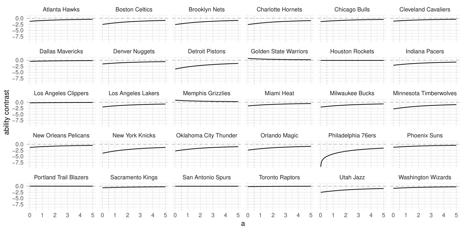 Figure 1
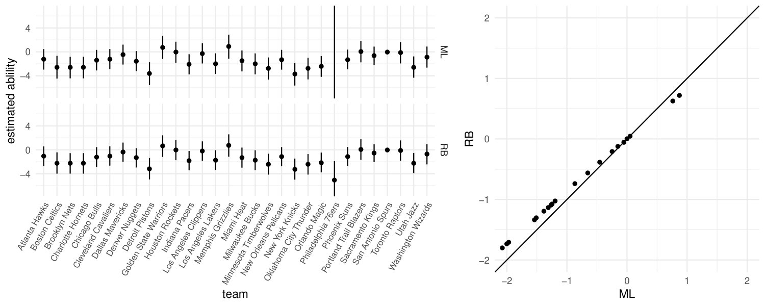 Figure 2
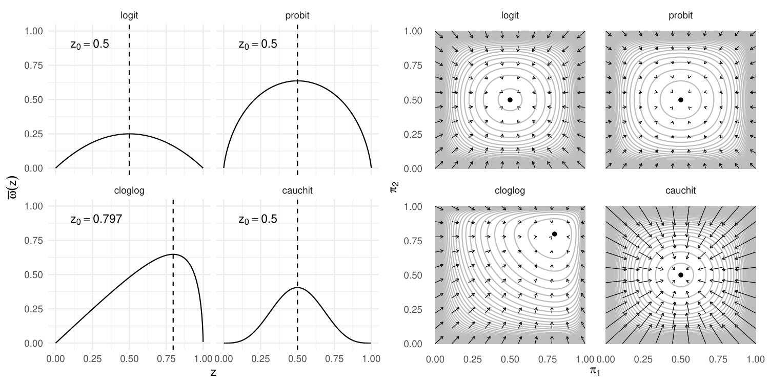 Figure 3
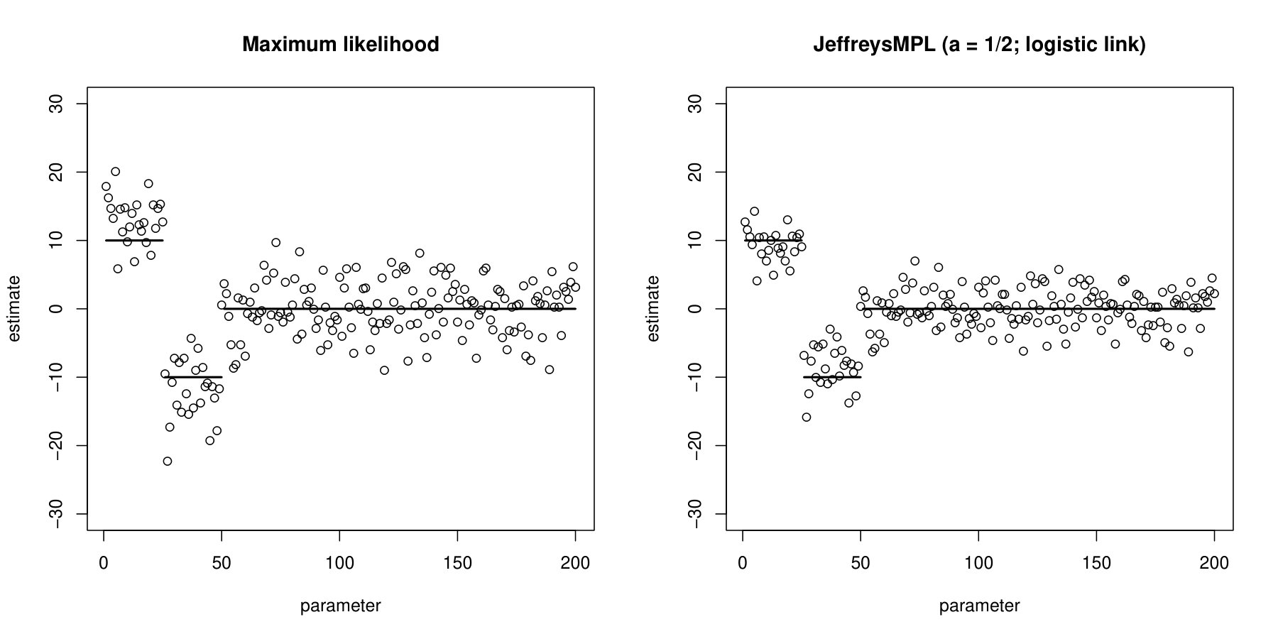 Figure 4
 Figure 5
| Link function | ||
|---|---|---|
| logit | ||
| probit | ||
| c-log-log | ||
| log-log | ||
| cauchit |
Peer Reviews
No public reviews on file for this paper yet. If you reviewed it on a platform where reviews are public (OpenReview, ICLR, NeurIPS, ICML), you can paste yours below so the community can read it here.
Code & Models
Videos
No videos yet. Explain this paper in a talk, walkthrough, or lecture? Add one.
Jeffreys-prior penalty, finiteness and shrinkage in
binomial-response generalized linear models
Ioannis Kosmidis
and
David Firth
Department of Statistics, University of Warwick
Coventry CV4 7AL, UK
and
The Alan Turing Institute
British Library, London NW1 2DB, UK
Abstract
Penalization of the likelihood by Jeffreys’ invariant prior, or by a positive power thereof, is shown to produce finite-valued maximum penalized likelihood estimates in a broad class of binomial generalized linear models. The class of models includes logistic regression, where the Jeffreys-prior penalty is known additionally to reduce the asymptotic bias of the maximum likelihood estimator; and also models with other commonly used link functions such as probit and log-log. Shrinkage towards equiprobability across observations, relative to the maximum likelihood estimator, is established theoretically and is studied through illustrative examples. Some implications of finiteness and shrinkage for inference are discussed, particularly when inference is based on Wald-type procedures. A widely applicable procedure is developed for computation of maximum penalized likelihood estimates, by using repeated maximum likelihood fits with iteratively adjusted binomial responses and totals. These theoretical results and methods underpin the increasingly widespread use of reduced-bias and similarly penalized binomial regression models in many applied fields.
Keywords: logit; probit; bias reduction; penalized likelihood; data separation; infinite estimate; working weight; Bradley-Terry model
1 Introduction
Logistic regression is one of the most frequently applied generalized linear models in statistical practice, both for inference about covariate effects on binomial probabilities, and for prediction. Consider realizations of independent binomial random variables with success probabilities and totals , respectively. Suppose that each is accompanied by a -dimensional covariate vector and that the model matrix with rows has full rank. A logistic regression model has
[TABLE]
where is the -dimensional parameter vector, and is the th element of ; if an intercept parameter is present in the model then the first column of is a vector of ones. The maximum likelihood estimator of in (1) maximizes the log-likelihood
[TABLE]
Albert & Anderson (1984) categorized the possible settings for the sample points , , into complete separation, quasi-complete separation and overlap. Specifically, if there exists a vector such that for all with and for all with , then there is complete separation in the sample points; if there exists a vector such that for all with and for all with , then there is quasi-complete separation in the sample points; and if neither complete nor quasi-complete separation is present, then the sample points overlap. Albert & Anderson (1984) showed that separation is necessary and sufficient for the maximum likelihood estimate to have at least one infinite-valued component. A parallel result appears in Silvapulle (1981), where it is shown that if in (1) is any strictly increasing distribution function such that and are convex, and , then the maximum likelihood estimate has all components finite if and only if there is overlap.
When data separation occurs, standard maximum-likelihood estimation procedures, such as iteratively reweighted least squares (Green, 1984), can be numerically unstable due to the occurrence of large parameter values as the procedures attempt to maximize (2). In addition, inferential procedures that directly depend on the estimates and the estimated standard errors, such as Wald tests, can give misleading results. For a recent review of such problems and some solutions, see Mansournia et al. (2018).
Firth (1993) showed that if the logistic regression likelihood is penalized by Jeffreys’ invariant prior, then the resulting maximum penalized likelihood estimator has bias of smaller asymptotic order than that of the maximum likelihood estimator in general. Specifically, for logistic regressions the reduced-bias estimator results from maximization of
[TABLE]
with , and where is the working weight for the th observation with . Heinze & Schemper (2002), in extensive numerical studies, observed that the reduced-bias estimates have finite values even when data separation occurs. Based on an argument about parameter-dependent adjustments to and stemming from the form of the gradient of (3), Heinze & Schemper (2002) conjectured that finiteness of the reduced-bias estimates holds for every combination of data and logistic regression model. Heinze & Schemper (2002) also observed that the reduced-bias estimates are typically smaller in absolute value than the corresponding maximum likelihood estimates, when the latter are finite. These observations are in agreement with the asymptotic bias of the maximum likelihood estimator in logistic regressions being approximately collinear with the parameter vector (see, for example, Cordeiro & McCullagh, 1991).
Example 1 illustrates the finiteness and shrinkage properties of the maximum penalized likelihood estimator in the context of estimating the strength of NBA basketball teams using a Bradley-Terry model (Bradley & Terry, 1952).
Example 1**:**
Suppose that when team beats team , and , otherwise. The Bradley-Terry model assumes that the contest outcome is the realization of a Bernoulli random variable with probability , and that the outcomes for the available contests are independent. The Bradley-Terry model is a logistic regression with probabilities as in (1), for the particular matrix whose rows are indexed by contest identifiers and whose general element is . Here, is the Kronecker delta, with value one when and zero otherwise. The parameter can be thought as measuring the ability or strength of team . Only contrasts are estimable, and an identifiable parameterization can be achieved by setting one of the abilities to zero. See, for example, Agresti (2013, § 11.6) for a general discussion of the model.
We use the Bradley-Terry model to estimate the ability of basketball teams from game outcomes in the regular season of the 2014–2015 NBA conference. For illustrative purposes, we use only the games that took place before 3 December 2014, up to which date the Philadelphia 76ers had recorded 17 straight losses and no win. The dataset was obtained from www.basketball-reference.com and is also available as part of the Supplementary Material. The ability of the San Antonio Spurs, the champion team of the 2013–2014 conference, is set to zero, so that each is the contrast of the ability of team with San Antonio Spurs. The model is estimated via iteratively reweighted least squares, as implemented in the glm function of R (R Core Team, 2020) with default settings for the optimization. No warning or error was returned during the fitting process.
The top panel in the left plot of Figure 1 shows the reported maximum likelihood estimates of the contrasts, along with their corresponding nominally individual Wald-type confidence intervals. The contrast for Philadelphia 76ers stands out in the output from glm with a value of and a corresponding estimated standard error of . These values are in fact representations of and , respectively, as confirmed by the detect_separation method of the brglm2 R package (Kosmidis, 2020), which implements separation-detection algorithms from a 2007 University of Oxford Department of Statistics PhD thesis by K. Konis. The data are separated, with the maximum likelihood estimates for all teams being finite except that for Philadelphia 76ers, which is minus infinity. A particularly worrying side-effect of data separation here is that if the computer output is used naively, a Wald test for difference in ability between Philadelphia 76ers and San Antonio Spurs results in no apparent evidence of a difference, which is counter intuitive given that the former had no wins in 17 games and the latter had 13 wins in 17 games. In contrast, the reduced-bias estimates in the bottom panel of the left of Figure 1 all have finite values and finite standard errors. The right plot in Figure 1 illustrates the shrinkage of the reduced-bias estimates towards zero that has also been discussed in a range of different settings, for example in Heinze & Schemper (2002) and Zorn (2005).
The apparent finiteness and shrinkage properties of the reduced-bias estimator, coupled with the fact that the estimator has the same first-order asymptotic distribution as the maximum likelihood estimator, are key reasons for the increasingly widespread use of Jeffreys-prior penalized logistic regression in applied work. At the time of writing, Google Scholar records approximately 2700 citations of Firth (1993), more than half of which are from 2015 or later. The list of application areas is diverse, including for example agriculture and fisheries research, animal and plant ecology, criminology, commerce, economics, psychology, health and medical sciences, politics and many more. The particularly strong uptake of the method in health and medical sciences, and politics stems largely from the works of Heinze & Schemper (2002) and Zorn (2005), respectively. The reduced-bias estimator is also implemented in dedicated open-source software, such as the brglm2 (Kosmidis, 2020) and logistf (Heinze & Ploner, 2018) R packages, and it has now become part of textbook treatments of logistic regression; see, for example, Agresti (2013, § 7.4), or Hosmer et al. (2013, § 10.3).
However, a definitive theoretical account of the empirically evident finiteness and shrinkage properties has yet to appear in the literature. Such a formal account is much needed, particularly in light of recent advances that demonstrate benefits of the reduced-bias estimator in wider contexts than the ones for which it was originally developed. An example of such an advance is Lunardon (2018), which explores the performance of bias reduction in stratified settings and shows that bias reduction is particularly effective for inference about a low-dimensional parameter of interest in the presence of high-dimensional nuisance parameters. For the estimation of high-dimensional logistic regression models with , , experiments reported in the supplementary information of Sur & Candès (2019) (see, also, Section S3.3 in the Supplementary Material) show that bias reduction performs similarly to their newly proposed method, and markedly better than maximum likelihood. These new theoretical and empirical results justify and motivate use of the reduced-bias estimator in even more complex applied settings than the one covered by the framework of Firth (1993); in such settings, more involved methods such as modified profile likelihoods (see, for example Sartori, 2003) and approximate message-passing algorithms (see, for example Sur & Candès, 2019) have also been proposed for recovering inferential accuracy.
This paper formally derives the finiteness and shrinkage properties of reduced-bias estimators for logistic regressions under only the condition that model matrix has full rank. We also provide geometric insights on how penalized likelihood estimators shrink towards zero, and discuss the implications of finiteness and shrinkage in inference, especially in hypothesis tests and confidence regions using Wald-type procedures.
It is shown how the results extend in a direct way to other commonly-used link functions, such as the probit, log-log, complementary log-log and cauchit, whenever the Jeffreys prior is used as a likelihood penalty. The work presented here thus complements earlier work of Ibrahim & Laud (1991) and especially Chen et al. (2008), which studies the same models from a Bayesian perspective. Here we study the behaviour of the posterior mode and thereby derive results that add to those earlier findings, whose focus was instead on important Bayesian aspects such as propriety and moments of the posterior distribution.
The results in this paper also readily extend to situations where penalized log-likelihoods of the form
[TABLE]
are used, with allowed to take values other than . Such penalized log-likelihoods have proved useful in prediction contexts, where the value of can be tuned to deliver better estimates of the binomial probabilities; and they are the subject of ongoing research (see, for example, Elgmati et al., 2015; Puhr et al., 2017). The repeated maximum likelihood fits procedure with iteratively adjusted binomial responses and totals, derived in Section 4, maximizes for general binomial-response generalized linear models and any .
2 Logistic regression
2.1 Preamble
Results on finiteness and shrinkage of the maximum penalized likelihood estimator are derived first for logistic regression, which is the leading case in applications and also the case for which maximum penalized likelihood, with Jeffreys-prior penalty, coincides with asymptotic bias reduction. These results provide a platform for the generalization to link functions other than logit in Section 3.
2.2 Finiteness
Let be at , , where is a path in such that as , with having at least one infinite component. Theorem 1 below describes the limiting behaviour of the determinant of the expected information matrix as diverges to infinity, only under the assumption that is of full rank. An important implication of Theorem 1 is Corollary 1 which shows that the reduced-bias estimators for logistic regressions are always finite. These new results formalize a sketch argument made in Firth (1993, § 3.3).
Theorem 1**:**
Suppose that has full rank. Then .
Corollary 1**.**
Suppose that has full rank. The vector that maximizes has all of its components finite.
The proofs of Theorem 1 and Corollary 1 are given in the Supplementary Material.
Corollary 1 also holds for any fixed in (4). As a result, the maximum penalized likelihood estimators from the maximization of in (4) have finite components, for any .
Despite its practical utility, the finiteness of the reduced-bias estimator results in some notable, and perhaps undesirable, side-effects on Wald-type inferences based on the reduced-bias estimator that have been largely overlooked in the literature. The finiteness of implies that the estimated standard errors , calculated as the square roots of the diagonal elements of the inverse of , are also always finite. Since are realizations of binomial random variables, there is only a finite number of values that the estimator can take for any given . Hence, there will always be a parameter vector with large enough components that the usual Wald-type confidence intervals , or confidence regions in general, will fail to cover regardless of the nominal level that is used. This has also been observed in the complete enumerations of Kosmidis (2014) for proportional odds models which are extensions of logistic regression to ordinal responses; and it is also true when the penalized likelihood is profiled for the construction of confidence intervals, as is proposed, for example, in Heinze & Schemper (2002), and in Bull et al. (2007) for multinomial regression models.
2.3 Shrinkage
The following theorem is key when exploring the shrinkage properties of the reduced-bias estimator that have been illustrated in Example 1.
Theorem 2**:**
Suppose that has full rank. Then
- i)
The function is globally maximized at .
- ii)
If , then is log-concave on .
A complete proof of Theorem 2 is in the Supplementary Material. Part i) also follows directly from Chen et al. (2008, Theorem 1).
Consider estimation by maximization of the penalized log-likelihood in (4) for and with . Let and be the maximizers of and , respectively and and the corresponding estimated -vectors of probabilities. Then, by the concavity of , the vector is closer to than is , in the sense that lies within the hull of that convex contour of containing . With the specific values and the last result refers to maximization of the likelihood penalized by Jeffreys prior and to maximization of the un-penalized likelihood, respectively. Hence, use of reduced-bias estimators for logistic regressions has the effect of shrinking towards the model that implies equiprobability across observations, relative to maximum likelihood. Shrinkage here is according to a metric based on the expected information matrix rather than to Euclidean distance. Hence, the reduced-bias estimates are only typically, rather than always, smaller in absolute value than the corresponding maximum likelihood estimates.
If the determinant of the inverse of the expected information matrix is considered as a generalized measure of the asymptotic variance, then the estimated generalized asymptotic variance at the reduced-bias estimates is always smaller than the corresponding estimated variance at the maximum likelihood estimates. Hence approximate confidence ellipsoids, based on asymptotic normality of the reduced-bias estimator, are reduced in volume.
3 Non-logistic link functions
3.1 Preamble
The results here generalize Sections 2.2 and 2.3 beyond the logit link, still for estimators from penalized likelihoods of form (4). For non-logistic links, such estimators no longer coincide with the bias-reduced estimator of Firth (1993).
3.2 Finiteness
The results in Theorem 1 and Corollary 1 readily extend to more link functions than the logistic. Specifically, if in model (1) is replaced by an at least twice differentiable and invertible function , then the expected information matrix has again the form but with working weights where and . If the link function is such that as diverges to either or , then the proofs of Theorem 1 and Corollary 1 in the Supplementary Material apply unaltered to show that and, when the penalty is a positive power of Jeffreys’ invariant prior, the maximum penalized likelihood estimates have finite components. The logit, probit, complementary log-log, log-log and cauchit links are some commonly-used link functions for which . The functions and for each of the above link functions are shown in Table 1.
3.3 Shrinkage
Let . If the link function is such that is maximized at some value , then the same arguments as in the proof of result i) in Theorem 2 can be used to show that is globally maximized at . The left plot of Figure 2 illustrates that this condition is satisfied for the logit, probit, log-log, and complementary log-log link functions. If , then the maximum of is achieved at , where . In addition, directly from the proof of Theorem 2, a sufficient condition for the log-concavity of for non-logit link functions is that is concave.
4 Maximum penalized likelihood as repeated maximum likelihood
The maximum penalized likelihood estimates, for full rank , can be computed by direct numerical optimization of the penalized log-likelihood in (4) or by using a quasi Newton-Raphson iteration as in Kosmidis & Firth (2010). Nevertheless, the particular form of the Jeffreys prior allows the convenient computation of penalized likelihood estimates by leveraging readily available maximum-likelihood implementations for binomial-response generalized linear models.
If in model (1) is replaced by any invertible function that is at least twice differentiable, then differentiation of with respect to gives that the penalized likelihood estimates are the solutions of
[TABLE]
where , , , and with . The quantity is the th diagonal element of the ‘hat’ matrix .
If we temporarily omit the observation index and suppress the dependence of the various quantities on , the derivatives of are the derivatives of the binomial log-likelihood with link function , after adjusting the binomial response to . Hence, the penalized likelihood estimates can be conveniently computed through repeated maximum-likelihood fits, where each repetition consists of two steps: P1) the adjusted responses are computed at the current parameter values; and P2) the maximum likelihood estimates of are computed at the current value of the adjusted responses.
However, depending on the sign and magnitude of , the adjusted response can be either negative or greater than the binomial total . In such cases, standard implementations of maximum likelihood are either unstable or report an error. This is because the binomial log-likelihood is not necessarily concave when or for at least one observation, when a link function with concave and is used. Logit, probit, log-log and complementary log-log are link functions of this kind. See, for example, Pratt (1981, § 5) for results and discussion on concavity of the log-likelihood.
Such issues with the use of repeated maximum-likelihood fits can be avoided by noting that expression (5) results if, in the derivatives of the log-likelihood, and are replaced, respectively, by their adjusted versions
[TABLE]
Here is some arbitrarily chosen function of . The following theorem identifies one function for which .
Theorem 3**:**
Let be 1 if holds and 0 otherwise. If , then .
The proof of Theorem 3 is given in the Supplementary Material, which also provides pseudo-code (see Algorithm S1) and R code for Algorithm JeffreysMPL, which implements repeated maximum-likelihood fits to maximize the for any supplied and link function .
The variance-covariance matrix of the penalized likelihood estimator can be obtained as , where is the upper triangular matrix from the QR decomposition of at the final iteration of the procedure. That decomposition is a by-product of JeffreysMPL.
If, in addition to full rank , we require that has a column of ones and is a unimodal density function, then it can be shown that if the starting value of the parameter vector in the repeated maximum-likelihood fits procedure has finite components, then the values of computed in step P2 will also have finite components at all repetitions. This is because, with a column of ones in the full rank , the adjusted responses and totals in (6) satisfy , and hence maximum likelihood estimates with infinite components are not possible. The strict inequalities hold because, under the aforementioned conditions, and is positive definite for with finite components. Then, Magnus & Neudecker (1999, Chapter 11, Theorem 4) on bounds for the Rayleigh quotient gives the inequality , where is the minimum eigenvalue of .
The repeated maximum-likelihood fits procedure has the correct fixed point even if, at step P2, full maximum-likelihood estimation is replaced by a procedure that merely increases the log-likelihood, such as a single step of iteratively reweighted least squares for the adjusted responses and totals. Firth (1992) suggested such a scheme for logistic regressions with . There is currently no conclusive result on whether full maximum-likelihood iteration with a reasonable stopping criterion is better or worse than, for example, one step of iteratively reweighted least squares, in terms of computational efficiency. A satisfactory starting value for the above procedure is the maximum likelihood estimate of , after adding a small positive constant and twice that constant to the actual binomial responses and totals, respectively.
Finally, for , repeated maximum-likelihood fits can be used to compute the posterior normalizing constant when implementing the importance sampling algorithm in Chen et al. (2008, § 5) for posterior sampling of the parameters of Bayesian binomial-response generalized linear models with the Jeffreys prior.
Section S3 of the Supplementary Material illustrates the evolution of adjusted responses and totals through the iterations of JeffreysMPL, for the first 6 games of Philadelphia 76ers in Example 1. Section S3 also computes the reduced-bias estimates for a logistic regression model with binary responses and covariates, as considered in Figure 2(b) of the supplementary information appendix of Sur & Candès (2019), and illustrates that such computation takes only a couple of seconds on a standard laptop computer.
5 Illustrations
The left plot of Figure 2 shows and for the various links. The plot for the log-log link is the reflection of the one for the complementary log-log through . As is apparent, is concave for the logit, probit and complementary-log-log links but not for the cauchit link. The right plot of Figure 2 visualizes the shrinkage induced by the penalization by Jeffreys’ invariant prior for the logit, probit, complementary log-log and cauchit links. For each link function, we obtain all possible fitted probabilities from a complete enumeration of a saturated model with , where , , and . The grey curves are the contours of . An arrow is drawn from each pair of estimated probabilities based on the maximum likelihood estimates to the corresponding pair of estimated probabilities based on penalized likelihood estimates, to demonstrate the induced shrinkage towards in accord to the results in Section 3. Despite the fact that is not concave for the cauchit link, the fitted probabilities still shrink towards . The plots in Figure 2 are invariant to the particular choice of and , as long as . For either maximum likelihood or maximum penalized likelihood, if the estimates of and are and for and , then the new estimates for any with are and , respectively. Hence, the fitted probabilities will be identical.
Another illustration of finiteness and shrinkage follows from Example 1. Figure 3 shows the paths of the team ability contrasts as varies from [math] to . The estimates are obtained using JeffreysMPL, starting at the maximum likelihood estimates of the ability contrasts after adding and to the actual responses and totals, respectively. In accord with the theoretical results in Section 2.2, the estimated ability contrasts are finite for every ; and, as expected from the results in Section 2.3, shrinkage towards equiprobability becomes stronger as increases.
6 Concluding remarks
A recent stream of literature investigates the use of the coefficient path defined by maximization of the penalized log-likelihood (4) for the prediction of rare events through logistic regression. Elgmati et al. (2015) study that path for , and propose to take to be around , in order to handle issues related to infinite estimates, and they obtain predicted probabilities that are less biased than those based on the reduced-bias estimates (). More recently, Puhr et al. (2017) proposed two new methods for the prediction of rare events, and performed extensive simulation studies to compare performance with various methods, including maximum penalized likelihood with and .
The coefficient path can be computed efficiently by using repeated maximum-likelihood fits with “warm” starts. For a grid of values with , JeffreysMPL (Algorithm S1 in the Supplementary Material) is first applied with to get the maximum penalized likelihood estimates ; then, JeffreysMPL is applied again with with starting values , and so on, until has been computed. This process supplies JeffreysMPL with the best available starting values, as the algorithm walks through the grid. The finiteness of the components of and the shrinkage properties described in Sections 2.3 and 3 contribute to the stability of the overall process. The properties of the coefficient path for inference and prediction from binomial regression models, and the development of general procedures for selecting , are interesting, open research topics.
Kenne Pagui et al. (2017) develop a method that can reduce the median bias of the components of the maximum likelihood estimator. According to the results therein, median bias reduction for one-parameter logistic regression models is equivalent to maximizing (4) with . Hence, the results in Section 2 also establish the finiteness of the estimate from median bias reduction in one-parameter logistic regression, and that the induced shrinkage to equiprobability will be less strong than penalization by the Jeffreys prior. Kenne Pagui et al. (2017) observed such properties in numerical studies for . When , though, median bias reduction is no longer equivalent to maximizing (4) with .
7 Acknowledgments
Ioannis Kosmidis and David Firth are supported by The Alan Turing Institute under the EPSRC grant EP/N510129/1. David Firth was partly supported also by EPSRC programme EP/K014463/1, Intractable Likelihood: New Challenges from Modern Applications.
8 Supplementary material
The Supplementary Material is available for download at http://www.ikosmidis.com/files/finiteness-jeffreys-supplementary-v1.4.zip and includes: a document with proofs for Theorems 1, 2, 3 and Corollary 1; Algorithm S1, and some additional numerical results; and R code and data to reproduce all of the numerical work and graphs.
The reference list from the paper itself. Each links out to its DOI / PubMed record.
- 1Agresti (2013) Agresti, A. (2013). Categorical Data Analysis . Hoboken, NJ: John Wiley & Sons, 3rd ed.
- 2Albert & Anderson (1984) Albert, A. & Anderson, J. (1984). On the existence of maximum likelihood estimates in logistic regression models. Biometrika 71 , 1–10.
- 3Bradley & Terry (1952) Bradley, R. A. & Terry, M. E. (1952). Rank analysis of incomplete block designs: I. The method of paired comparisons. Biometrika 39 , 324–345.
- 4Bull et al. (2007) Bull, S. B. , Lewinger, J. B. & Lee, S. S. F. (2007). Confidence intervals for multinomial logistic regression in sparse data. Statistics in Medicine 26 , 903–918.
- 5Chen et al. (2008) Chen, M.-H. , Ibrahim, J. G. & Kim, S. (2008). Properties and implementation of Jeffreys’s prior in binomial regression models. Journal of the American Statistical Association 103 , 1659–1664.
- 6Cordeiro & Mc Cullagh (1991) Cordeiro, G. M. & Mc Cullagh, P. (1991). Bias correction in generalized linear models. Journal of the Royal Statistical Society, Series B: Methodological 53 , 629–643.
- 7Elgmati et al. (2015) Elgmati, E. , Fiaccone, R. L. , Henderson, R. & Matthews, J. N. S. (2015). Penalised logistic regression and dynamic prediction for discrete-time recurrent event data. Lifetime Data Analysis 21 , 542–560.
- 8Firth (1992) Firth, D. (1992). Bias reduction, the Jeffreys prior and GLIM. In Advances in GLIM and Statistical Modelling: Proceedings of the GLIM 92 Conference, Munich , L. Fahrmeir, B. Francis, R. Gilchrist & G. Tutz, eds. New York: Springer.
