Kinematics of Subclusters in Star Cluster Complexes: Imprint of their Parental Molecular Clouds
M. S. Fujii

TL;DR
This study uses N-body simulations based on hydrodynamic models to explore how turbulent molecular clouds influence the formation and kinematics of star cluster complexes, matching observed data from the Carina Nebula and NGC 2264.
Contribution
It introduces a simulation approach linking molecular cloud turbulence to the formation of subclusters in star complexes, aligning results with Gaia observations.
Findings
Simulated inter-clump velocity dispersions match Gaia data.
Estimated parental cloud masses are consistent with observations.
Results support turbulence-driven subclustering in star formation.
Abstract
Star cluster complexes such as the Carina Nebula can have formed in turbulent giant molecular clouds. We perform a series of -body simulations starting from subclustering initial conditions based on hydrodynamic simulations of turbulent molecular clouds. These simulations finally result in the formation of star cluster complexes consisting of several subclusters (clumps). We obtain the inter-clump velocity distribution, the size of the region, and the mass of the most massive cluster in our simulated complex and compare the results with observed ones (the Carina Nebula and NGC 2264). The one-dimensional inter-clump velocity dispersion obtained from our simulations is and km s for the Carina- and NGC 2264-like models, respectively, which are consistent with those obtained from Gaia Data Release 2: 2.35 and 0.99 km s for the Carina Nebula and NGC…
Click any figure to enlarge with its caption.
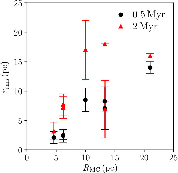 Figure 1
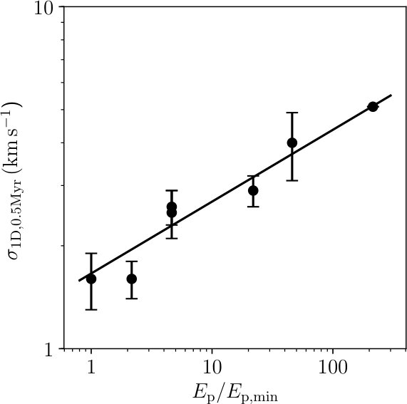 Figure 2
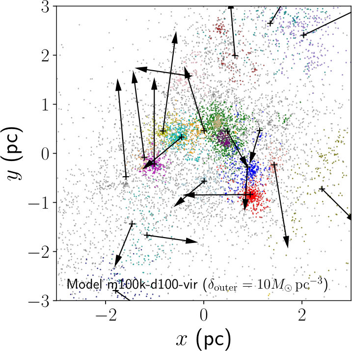 Figure 3
 Figure 4
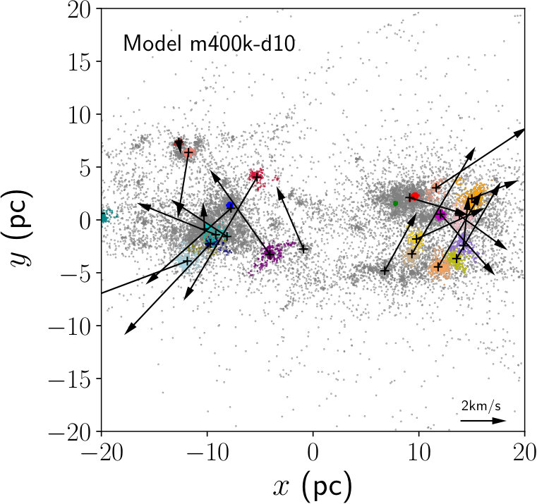 Figure 5
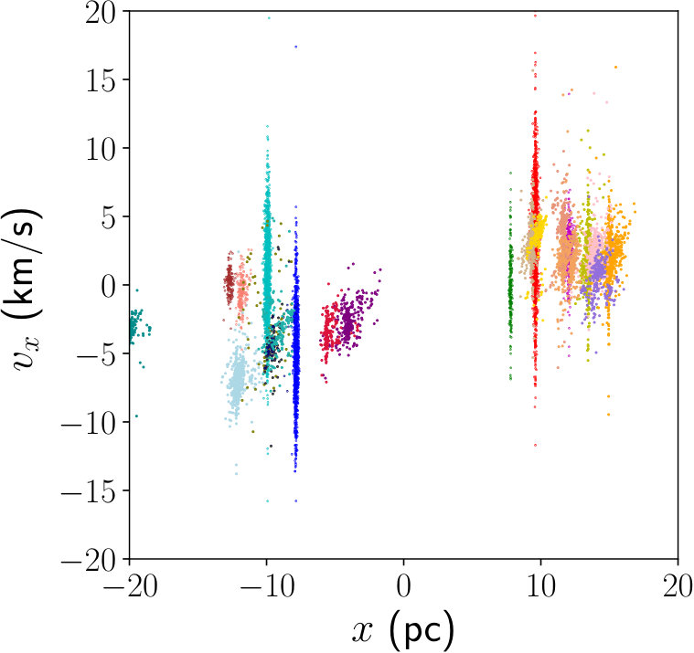 Figure 6
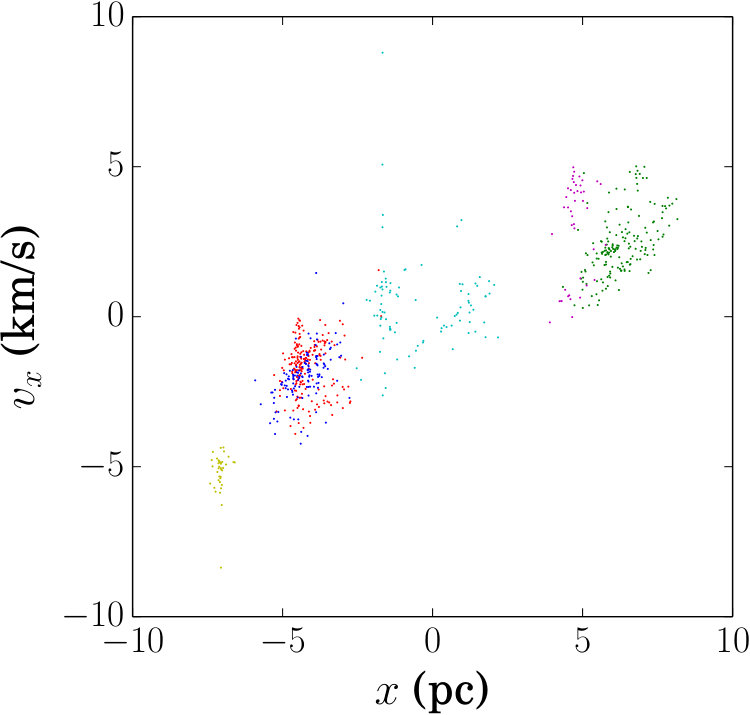 Figure 7
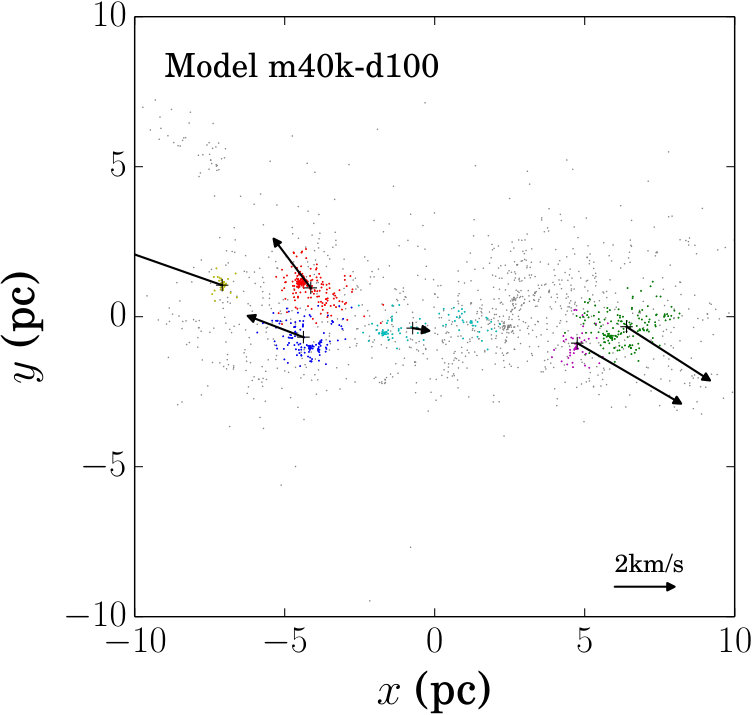 Figure 8
| Model | (pc) | (km s-1) | ||
|---|---|---|---|---|
| m1M-d100 | 1 | 1000 | 13.3 | 19.6 |
| m400k-d100 | 3 | 400 | 10.0 | 14.4 |
| m100k-d100(-vir) | 5 | 100 | 6.2 | 9.12 |
| m40k-d100 | 10 | 40 | 4.6 | 6.70 |
| m400k-d10 | 3 | 400 | 21.0 | 9.92 |
| m100k-d10 | 6 | 100 | 13.3 | 6.23 |
| Model | (km s-1) | (pc) | |||
|---|---|---|---|---|---|
| 0.5 Myr | |||||
| m1M-d100 | 151 | 5.1 | 8.3 | ||
| m400k-d100 | |||||
| m100k-d100 | |||||
| m100k-d100-vir | |||||
| m40k-d100 | |||||
| m400k-d10 | |||||
| m100k-d10 | |||||
| 2 Myr | |||||
| m1M-d100 | 108 | 4.5 | 18 | ||
| m400k-d100 | |||||
| m100k-d100 | |||||
| m100k-d100-vir | |||||
| m40k-d100 | |||||
| m400k-d10 | |||||
| m100k-d10 | |||||
| Name | Age | (km s-1) | (pc) | Ref. | |||
|---|---|---|---|---|---|---|---|
| Carina | 0.5 | 28 | 16 | 2.35 | 11.2 | 4.3 | (1), (2), (3) |
| NGC 2264 | 3 | 1.1 | 8 | 0.99 | 2.53 | 0.15 | (3), (4), (5) |
| Changed parameters | (km s-1) | (pc) | ||
|---|---|---|---|---|
| 0.5 Myr | ||||
| Standard | ||||
| pc-3 | ||||
| 2 Myr | ||||
| Standard | ||||
| pc-3 | ||||
Peer Reviews
No public reviews on file for this paper yet. If you reviewed it on a platform where reviews are public (OpenReview, ICLR, NeurIPS, ICML), you can paste yours below so the community can read it here.
Videos
No videos yet. Explain this paper in a talk, walkthrough, or lecture? Add one.
Kinematics of Subclusters in Star Cluster Complexes:
Imprint of their Parental Molecular Clouds
M. S. Fujii1
1Department of Astronomy, Graduate School of Science, The University of Tokyo, 7-3-1 Hongo, Bunkyo-ku, Tokyo, 113-0033, Japan E-mail: [email protected]
(Accepted . Received ; in original form 1988 October 11)
Abstract
Star cluster complexes such as the Carina Nebula can have formed in turbulent giant molecular clouds. We perform a series of -body simulations starting from subclustering initial conditions based on hydrodynamic simulations of turbulent molecular clouds. These simulations finally result in the formation of star cluster complexes consisting of several subclusters (clumps). We obtain the inter-clump velocity distribution, the size of the region, and the mass of the most massive cluster in our simulated complex and compare the results with observed ones (the Carina Nebula and NGC 2264). The one-dimensional inter-clump velocity dispersion obtained from our simulations is and km s*-1* for the Carina- and NGC 2264-like models, respectively, which are consistent with those obtained from Gaia Data Release 2: 2.35 and 0.99 km s*-1* for the Carina Nebula and NGC 2264, respectively. We estimate that the masses of the parental molecular clouds for the Carina Nebula and the NGC 2264 are and , respectively.
keywords:
methods: numerical — galaxies: star clusters: general — Galaxy: open clusters and associations: general — Galaxy: open clusters and associations: individual: Carina, NGC 2264
††pagerange: Kinematics of Subclusters in Star Cluster Complexes: Imprint of their Parental Molecular Clouds–4††pubyear: 2018
1 Introduction
Star clusters are often born in a hierarchical structure which consists of several subclusters (hereafter clumps). One of the biggest systems is the Carina Nebula, which include several star clusters and smaller clumps (Feigelson et al., 2011; Kuhn et al., 2014). Such “star cluster complexes” are considered to have formed via the gravitational collapse of giant molecular clouds with turbulence (McKee & Ostriker, 2007, and references therein). The formation of stars and star clusters in turbulent molecular clouds have been tested using numerical simulations (Bonnell et al., 2008; Bate, 2012; Krumholz et al., 2012b; Federrath & Klessen, 2012; Fujii & Portegies Zwart, 2015; Fujii, 2015; Fujii & Portegies Zwart, 2016). In these studies, hierarchical structure formation has been confirmed.
Star clusters are initially embedded in their parental molecular clouds (Lada & Lada, 2003), but once massive stars formed, the gas is expelled by gas expulsion such as ionization, stellar winds, and supernovae explosions. As a result, the embedded clusters are expected to expand. This expansion has also been studied using numerical simulations (Pfalzner, 2009; Pelupessy & Portegies Zwart, 2012) and also by observations (Gouliermis, 2018; Kuhn et al., 2018).
Not only star clusters, star cluster complexes have also been suggested to expand by numerical simulations. Fujii & Portegies Zwart (2015) performed a series of simulations of star cluster complexes forming in turbulent molecular clouds. They suggested that star cluster complexes also expand although some subclusters (hereafter, clumps) merge and evolve to more massive clusters within a few Myr (see also Fujii, 2015; Fujii & Portegies Zwart, 2016). However, the relative velocity among clumps in star cluster complexes was not studied in their work.
Observational studies on the kinematics of star cluster complexes require an accurate velocity measurement. Thanks to Gaia Data Release 2 (Gaia Collaboration et al., 2018), the proper motions of individual stars in young star clusters and associations are now available. This data allows us to study the kinematics of star cluster complexes. Kuhn et al. (2018) measured inter clump velocities for some star cluster complexes such as the Carina Nebula. They reported an expansion of star cluster complexes as well as that of young star clusters.
In this paper, we measure the velocity structure among clumps in star cluster complexes using the results of our numerical simulations (Fujii, 2015; Fujii & Portegies Zwart, 2016) and additional new simulations. We connect the current spacial and velocity distributions of clumps in star cluster complexes to their parental molecular clouds and estimate the properties of the parental molecular clouds.
2 Methods
2.1 Numerical Simulations
We use the results of Fujii & Portegies Zwart (2016) and also perform additional simulations for some models. Here, we briefly summarize the methods used in this study (see also Fujii, 2015; Fujii & Portegies Zwart, 2016).
First, we perform hydrodynamic simulations for molecular clouds using a smoothed-particles hydrodynamics (SPH) code, Fi (Hernquist & Katz, 1989; Gerritsen & Icke, 1997; Pelupessy et al., 2004; Pelupessy, 2005) with the Astronomical Multipurpose Software Environment (AMUSE) (Portegies Zwart et al., 2009, 2013; Pelupessy et al., 2013)111see http://amusecode.org/.. We set-up the initial conditions of the molecular clouds using AMUSE following Bonnell et al. (2003). We adopt isothermal (30K) homogeneous spheres and give a divergence-free random Gaussian velocity field with a power spectrum (Ostriker et al., 2001; Bonnell et al., 2003). The spectral index of appears in the case of compressive turbulence (Burgers turbulence), and recent observations of molecular clouds (Heyer & Brunt, 2004), and numerical simulations (Federrath et al., 2010; Roman-Duval et al., 2011; Federrath, 2013a) also suggested values similar to . We adopt the mass and density of the molecular clouds as parameters.
In Table 1, the initial conditions of molecular clouds are summarized. The model names represent the initial mass and density; for example, m400k and d100 indicate a mass of and a density of pc cm*-3* assuming that the mean weight per particle is . We adopt 10 and pc*-3* (170 and 1700 cm*-3*) for the density and , , , and for the mass. While the density of our initial conditions is 170–1700 cm*-3*, observed density of molecular clouds is 100–500 cm*-3* (Heyer & Dame, 2015). For models m1M-d100, m400k-d100, and m400k-d10, we use the results obtained in Fujii & Portegies Zwart (2015). We also perform simulations for additional models m100k-d100, m40k-d100, and m100k-d10. We set the kinetic energy () to be equal to the absolute value of the potential energy (). With this setting, the system is initially super-virial. For comparison, we test a model the same as model m100k-d100, but (model m100k-d100-vir).
After 0.9 free-fall time of the initial condition, we stop the SPH simulations (0.75 and 2.4 Myr for d100 and d10 models, respectively) and convert a part of the gas particles to stellar particles using the following procedure. We assume a local star formation efficiency (SFE), which depends on the local gas density , given by
[TABLE]
where is a coefficient which controls the star formation efficiency and a free parameter in our simulations. We adopt . This SFE is motivated by the result that the star formation rate scales with free-fall time (Krumholz et al., 2012a; Federrath, 2013b). Using this equation, we calculate the local SFE for each gas particle. Following it, we choose gas particles which should be converted to stellar particles. For the selected gas particles, we randomly assign stellar masses following a Salpeter mass function (Salpeter, 1955) with a lower and upper cut-off mass of 0.3 and 100 and converted the gas particle to a stellar particle. Although the mass does not locally conserved, the total mass globally conserves because the mean stellar mass is equal to the gas-particle mass in the SPH simulations. We assume that the velocity of the stellar particles are the same as that of their parent gas particles. With this assumption, the stellar system can take over the velocity field of their parental molecular cloud.
Resulting global SFE measured for the entire system was several %, but the local SFE for dense regions reaches %. In dense regions, the local SFE exceeds 0.5 and reaches 1.0 in the densest regions. We allow such a high local SFE following the results of previous studies, in which star formation was followed using sink particles and in dense stellar clumps stars were dominant (Moeckel & Bate, 2010; Kruijssen et al., 2012). The SFE of some models are summarized in Table 2 of Fujii & Portegies Zwart (2016).
We remove all residual gas particles and start -body simulations using the stellar distribution obtained from the SPH simulations. At this moment, the virial ratio (kinetic energy over potential energy) of the entire system is more than 0.5 (see Table 2 of Fujii & Portegies Zwart, 2016). The entire system, therefore, expands with time. In clumps, however, stars are dominant, and as a consequence they are initially bound. Such clumps survive, and some of them evolve to more massive clusters via mergers (see Fujii, 2015, for the details).
The -body simulations are performed using a sixth-order Hermite scheme (Nitadori & Makino, 2008) without gravitational softening. We perform up to 10 runs changing the random seeds for the turbulence. Runs with different random seeds result in different shapes of collapsing molecular clouds. The number of runs and the averaged total stellar mass of each model is summarized in Table 2.
2.2 Clump finding
At 0.5 Myr and 2 Myr from the beginning of the -body simulation, we identify clumps in the snapshots and measure their mass and velocity. Hereafter, we set the beginning of the -body simulation to be 0 Myr.
We use the HOP method (Eisenstein & Hut, 1998) in AMUSE for the clump finding. HOP is a clump finding algorithm using peak densities. In HOP, however, the connection to the nearest densest particle is set for each particle. This is for separating multiple clumps which exist in a region denser than a threshold density. One of basic parameters of HOP is the outer cut-off density (a parameter for the minimum density threshold of clumps), . We set , which is three times the half-mass density of the entire system. We first calculate the local density of each star using nearest stars. We set . Using the local densities, the stars are connected to the densest particles within nearest stars as a potential member of the clump. In some dense region may include multiple clumps. In such a case, the clump members can be separated to multiple clumps using the saddle density (). HOP finds multiple clumps using the connection and separate them using the saddle density threshold, . We adopt . We also set the peak density, . The peak density of each clump must be higher than . We tested some combinations of these parameters and confirmed that the inter-clump velocity dispersion does not strongly depend on the choice of the parameters. We summarize the results with different parameter sets in Appendix A.
If the mean density of the detected clump is less than , we repeat the same procedure for the clump, because the clump may consist of some sub-clumps. We set the minimum number of stars for a clump to be 50, but for models m40k-d10 and m100k-d10, we reduce it to 32 because their total mass is smaller than the other models, and as a result, the number of clumps are also small. The detected clumps have a mass-radius relation similar to that of observed clusters. We confirmed it in our previous papers (Fujii, 2015; Fujii & Portegies Zwart, 2016).
3 Results
We measure the center-of-mass velocity of the detected clumps with respect to the center-of-mass velocity of the all detected clumps. In the top panel of Fig. 1, we present the spacial distribution of stars and detected clumps for one of model m400k-d10 at 0.5 Myr. The initial mass and density of this model are and pc*-3*, respectively. We also show the velocity vector of each clump in the figure.
The averaged size (three-dimensional root-mean-square radius from the center-of-mass position) and one-dimensional velocity dispersion among clumps of this model are (pc) and (km s*-1*), respectively. These values are similar to those of the Carina Nebula; the two-dimensional root-mean-square radius and the one-dimensional velocity dispersion are 9.15 pc and km s*-1*, respectively (Kuhn et al., 2018). Considering the root-mean-square radius in our simulations is calculated in three dimension, the observed radius is scaled to be 11.2 pc. The entire system of this model is distributed in pc (see the top panel of Fig. 1). The Carina Nebula is also distributed on similar scale (see Fig. 13 in Kuhn et al., 2018).
The relation between the mass of the parental molecular clouds () and the most massive star cluster () was discussed in our previous study (Fujii & Portegies Zwart, 2015), and found that it follows:
[TABLE]
A similar relation is also found using radiation-hydrodynamic simulations with sink particles (Howard et al., 2018). Our results are roughly consistent with this relation. The mass of the most massive cluster (clump) would be an important parameter to discuss the parental molecular clouds. The mass of the most massive clump of model m400k-d10 is . The most massive cluster in the Carina Nebula is Trumpler 14, which has a mass of (Sana et al., 2010). The total stellar mass and gas dust mass of the Carina Nebula are estimated to be (Preibisch et al., 2011b) and , respectively, which are similar to those of model m400k-d10; and , respectively (see Tables 2 and 3).
In the bottom panel of Fig. 1, we present the position vs. velocity plot of individual stars in the detected clumps for this model. The clumps distribute within v_{x}\ {\raise-2.15277pt\hbox{\buildrel<\over{\sim}}}\ |10| km s*-1*, and this is consistent with that of the Carina Nebula (see Fig.12 in Kuhn et al., 2018). Here, we see the entire system is expanding.
At 0.5 and 2 Myr for each model, we calculate the average and standard deviation of the number (), one-dimensional velocity dispersion (), root-mean-square radius (), and maximum mass () of the detected clumps among the same models with different random seeds, and these results are summarized in Table 2. We, for comparison, summarize these values for Carina Nebula and NGC 2264 in Table 3. We here note that the inter-clump velocity dispersion measured in our simulations does not strongly depend on clump finding algorithms, because it is comparable to the velocity dispersion of all individual stars in the same region (see Appendix A).
While the velocity dispersion did not change much, the root-mean-square radius increased. This expansion is due to the gas expulsion. After we removed all gas particles, the virial ratio of this system is larger than (Fujii & Portegies Zwart, 2015; Fujii, 2015; Fujii & Portegies Zwart, 2016). The velocity dispersion among clumps depends on the initial condition of the molecular clouds. Higher mass or density result in a larger velocity dispersion. We found no clear differences even if we change the initial virial ratio of the molecular clouds (see models m100k-d100 and m100k-d100-vir). We discuss this point in Section 4.
In the top panel of Fig. 2, we present the spacial distribution of clumps with their velocity vectors for one of model m40k-d100, which has a size similar to NGC 2264 region. In order to compare with the results of Kuhn et al. (2018), we also present the position vs. velocity plots for these models in the bottom panels of this figure. In this case, we see a clear velocity gradient, which shows an expansion.
Since the age of NGC 2264 is estimated to be Myr (Venuti et al., 2017), we compare the results of this model at 2 Myr. The 1D velocity dispersion and root-mean-square radius at 2 Myr is km s*-1*, which is consistent with that of the NGC 2264 region (0.99 km s*-1*) (Kuhn et al., 2018). The size () of this model is pc at 2 Myr, which is similar to that of NGC 2264 (2.53 pc) (see Table 3 and Figure 13 of Kuhn et al., 2018). Model m100k-d10 also has a velocity dispersion comparable with model m40k-d100, but the size of model m100k-d10 is pc at 2 Myr, which is twice as large as that of model m40k-d100.
We also compare the maximum mass of the most massive cluster (S Mon) in NGC 2264 with the model. In order to obtain the mass of S Mon, we use the fraction of the number of samples summarized in Table 4 in Kuhn et al. (2018). According to the table, the number of samples for S Mon is 67, and the number of all samples in NGC 2264 is 516. If we assume that the fraction in the number of samples is the same as the mass fraction of S Mon, we estimate the mass of S Mon is from the total mass of NGC 2264 () (Piskunov et al., 2008). On the other hand, the mass of the most massive clump for model m40k-d100 is . The minimum value is comparable to the observation. We, therefore, estimate that NGC 2264 formed in a dense molecular cloud ( pc*-3* i.e., 1700 pc*-3*) with a mass of a few .
In our method, we assumed an instantaneous gas expulsion. In observed star cluster complexes, however, the gas mass is comparable to or large than stellar mass. In the Carina Nebula, for example, the estimated gas mass including dust is (Preibisch et al., 2011a), which is an order of magnitude larger than that of stellar mass, (Preibisch et al., 2011b). We, therefore, may overestimate the inter-cluster velocity dispersion in our simulations.
4 Discussion
Which initial parameter decides the inter-cluster velocity dispersion? In our simulations, the velocity dispersion depends on the potential energy of the initial molecular cloud. In Fig. 3, we present the relation between the potential energy of our initial molecular clouds and the inter-cluster velocity dispersion at 0.5 Myr. Since the velocity dispersion does not change much at 2 Myr, we fit a power-law function to this relation using a least-mean-square method and obtain (km s*-1*), where is the minimum among our models; specifically, for model m400k-d10.
In Fig. 4, we plot the relation between the initial size of the molecular cloud and the size of the resulting star cluster complexes at 0.5 and 2 Myr. At 0.5 Myr, the sizes of the complexes are correlated with those of the initial molecular cloud, but not in later time. This is because the expansion velocity of the complexes depends on the potential energy of the initial molecular cloud. Even if the initial size of the molecular cloud is the same, the expansion velocity can be different comparing models with different densities (see models m1M-d100 and m100k-d10).
In our study, we tested only initially spherical models. In the Orion A molecular cloud, however, stellar and proto-stellar clumps including the Orion Nebula Cluster is associated with a 50-pc scale filament (Megeath et al., 2016; Kounkel et al., 2018). In such a region, the initial molecular cloud might have been cylindrical (Bonnell et al., 2008), or a cloud-cloud collision might have triggered the star cluster formation (Fukui et al., 2018). In a large velocity dispersion of stars around the Integral Shaped Filament (Bally et al., 1987) associated with the Orion Nebula Cluster (Stutz & Gould, 2016), a magnetic field may play an important role to eject stars from the filament by the “slingshot” mechanism (Boekholt et al., 2017; Stutz, 2018).
5 Summary
We performed a series of -body simulations for the formation of star cluster complexes. Following the method in Fujii & Portegies Zwart (2015), we first performed SPH simulations of turbulent molecular clouds and then used the last snapshots to generate initial conditions for the -body simulations, in which stars are distributed in clumpy and filamental structures.
The one-dimensional inter-clump velocity dispersion obtained from our simulations is and km s*-1* for the Carina- and NGC 2264-like models, respectively, which are consistent with those obtained from Gaia Data Release 2, which are 2.35 and 0.99 km s*-1* for the Carina Nebula and NGC 2264. The simulated complexes expand with time. We also confirmed the size and the mass of the most massive clump in these models are consistent with the observations.
Our results suggest that the parental molecular cloud of NGC 2264 has a mass of and that Carina Nebula formed from a giant molecular cloud with a mass of , but the cloud density for NGC 2264 is estimated to be higher than that of the Carina Nebula. The inter-cluster velocity dispersion in our simulations, however, tends to be larger than that of observed star cluster complexes. This may be because we assumed an instantaneous gas expulsion, while observed star cluster complexes are still surrounded by molecular gas comparable or more massive than the total stellar mass.
Acknowledgments
The author thanks the referee, Richard Parker, for his useful comments. The author also thanks Jun Makino, Amelia Stutz, and Tjarda Boekholt for fruitful discussion. Numerical computations were carried out on Cray XC30 and XC50 CPU-cluster at the Center for Computational Astrophysics (CfCA) of the National Astronomical Observatory of Japan. The author was supported by The University of Tokyo Excellent Young Researcher Program. This work was supported by JSPS KAKENHI Grant Number 26800108 and 19H01933.
Appendix A Clump finding algorithm: HOP
We determined subclusters using HOP algorithm (Eisenhauer et al., 1998) in AMUSE. HOP is a clump finding algorithm based on density (e.g., Bertschinger & Gelb, 1991). In Friends-of-Friends (FoF) methods, multiple clumps connected with a bridging region can be detected as a clump (see e.g., Parker & Wright, 2018). In order to avoid this problem, in HOP, the connection to the nearest densest particle is set for each particle. This determine a local density peak to which each particle belongs.
Here, we briefly summarize how HOP works. HOP first calculates a local density of each particle using nearest particles, where is a parameter. The local density is determined by a spherical cubic spline kernel (Monaghan & Lattanzio, 1985). The recommended value in Eisenhauer et al. (1998) is . Next, the densest particle within nearest particles for each particle is determined. Here, is a parameter, and the recommended value in Eisenhauer et al. (1998) is . With this process, each particle is connected to a local density peak which the particle belongs to.
For the density, there are three parameters; peak density (), saddle density (), and outer density () thresholds. Density peaks higher than are detected as individual clumps. On the other hand, particles with a density lower than are excluded from clumps. Particles with a local density higher than are clump candidates.
In regions with a density higher than , several clumps can be included. In order to detect such clumps, is used. For a star in a density peak, if one of its nearest particles belongs to another density peak, then the averaged density of the two density peaks is calculated. If the averaged density is less than saddle density (), these two density peaks are detected as two clump. If not, they are treated as one clump. The recommended value for is 4.
The peak density () and saddle density are determined depending on . In Eisenhauer et al. (1998), and are recommended. The outer density threshold () should be chosen for each system, and can significantly change the result. In our study, we adopt three times of the half-mass density of the system (the density within a radius in which the half of the total mass is includes) as . The half-mass density in our models was typically 10–100 pc*-3* at 0.5 Myr and 1–10 pc*-3* at 2 Myr. For and , we adopt and , which values are higher than those recommended in Eisenhauer et al. (1998). In Eisenhauer et al. (1998), they applied this method to a cosmological -body simulations and chose the parameters. In our simulations, however, the density contrast in star cluster complexes would be higher than that of dark matter halos. We, therefore, chose a higher values for and . Even if we adopt density thresholds same as those adopted in Eisenhauer et al. (1998), the results did not change significantly (see Table 4).
We also tested a fixed value for . If we adopted pc*-3* for both 0.5 and 2 Myr, the number of clumps at 0.5 Myr was twice as large as that obtained using our standard setting. However, the velocity dispersion among the detected clumps was not much different from that obtained using the standard setting. In Figure 5, we present the positions and velocities of detected clumps with our standard setting (left) and pc*-3* (right). In the right panel, we see that a larger number of clumps with lower densities are identified because of the lower density threshold compared with our standard setting. We also find that some of the detected clumps in the right panel would not be identified as clumps by eye. Thus, a fixed outer density threshold for all models and all time does not work well, and we therefore adopt the mean density of the entire system as the outer density threshold rather than a fixed one.
For relatively large clumps, however, the determined velocities are consistent with those obtained from our standard settings. We also confirmed that the inter-clump velocity dispersion does not largely change even if we change the detection criteria. This is because the inter-clump velocity dispersion is similar to the velocity dispersion of all individual stars in the same region. We calculated the velocity dispersion within the , where we set it to be 3 pc. The velocity dispersion of all stars within 3 pc from the center of mass position of the complex is km s*-1* at Myr. At Myr, the velocity dispersion of all stars within pc) is km s*-1*. Thus, inter-clump velocity dispersion is an index relatively independent of clump finding algorithms.
We also changed the values of and from the recommended values in Eisenhauer et al. (1998). In our standard setting, we reduced the value of in order to detect clumps consisting of less than 50 particles. On the other hand, we increased to 32 in order to search peaks in slightly wider range of particles. However, the choice of and does not affect the results. In Table 4, we summarize the results using different values for HOP parameters.
The reference list from the paper itself. Each links out to its DOI / PubMed record.
- 1Bally et al. (1987) Bally J., Langer W. D., Stark A. A., Wilson R. W., 1987, Ap J , 312, L 45 · doi ↗
- 2Bate (2012) Bate M. R., 2012, MNRAS , 419, 3115 · doi ↗
- 3Bertschinger & Gelb (1991) Bertschinger E., Gelb J. M., 1991, Computers in Physics , 5, 164 · doi ↗
- 4Boekholt et al. (2017) Boekholt T. C. N., Stutz A. M., Fellhauer M., Schleicher D. R. G., Matus Carrillo D. R., 2017, MNRAS , 471, 3590 · doi ↗
- 5Bonnell et al. (2003) Bonnell I. A., Bate M. R., Vine S. G., 2003, MNRAS , 343, 413 · doi ↗
- 6Bonnell et al. (2008) Bonnell I. A., Clark P., Bate M. R., 2008, MNRAS , 389, 1556 · doi ↗
- 7Eisenhauer et al. (1998) Eisenhauer F., Quirrenbach A., Zinnecker H., Genzel R., 1998, Ap J , 498, 278 · doi ↗
- 8Eisenstein & Hut (1998) Eisenstein D. J., Hut P., 1998, Ap J , 498, 137 · doi ↗