Voting and Bribing in Single-Exponential Time
Du\v{s}an Knop, Martin Kouteck\'y, Matthias Mnich

TL;DR
This paper studies a bribery problem in voting systems, showing it is fixed-parameter tractable for many rules with a single-exponential time algorithm, resolving a long-standing open problem.
Contribution
It introduces the $ ext{R}$-Multi-Bribery problem and proves its fixed-parameter tractability for numerous voting rules, improving previous algorithms to single-exponential time.
Findings
Fixed-parameter tractability for many voting rules.
Single-exponential time algorithm for arbitrary costs.
Resolution of a long-standing open problem in computational social choice.
Abstract
We introduce a general problem about bribery in voting systems. In the -Multi-Bribery problem, the goal is to bribe a set of voters at minimum cost such that a desired candidate wins the perturbed election under the voting rule R. Voters assign prices for withdrawing their vote, for swapping the positions of two consecutive candidates in their preference order, and for perturbing their approval count to favour candidates. As our main result, we show that -Multi-Bribery is fixed-parameter tractable parameterized by the number of candidates for many natural voting rules , including Kemeny rule, all scoring protocols, maximin rule, Bucklin rule, fallback rule, SP-AV, and any C1 rule. In particular, our result resolves the parameterized complexity of -Swap Bribery for all those voting rules, thereby solving a long-standing open problem…
Click any figure to enlarge with its caption.
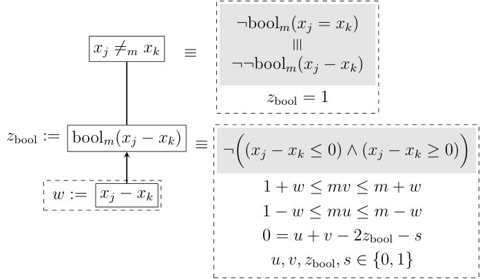 Figure 1
| problem name | specialization of -Multi-Bribery |
|---|---|
| -$Bribery | |
| -Manipulation | for , for |
| -CCAV/-CCDV | |
| -Swap Bribery | , , |
| -Shift Bribery | -Swap Bribery with for |
| -Support Brib. | |
| -Mixed Bribery | , |
| -Extension Bribery | if unranked, else ; , |
| -Possible Winner | reduce to -Swap Bribery [16, Thm. 2] |
| Dodgson Score | Condorcet-Swap Bribery with |
| Young Score | Condorcet-CCDV with |
| previous best result | new result | ||
| problem | run time / hardness | voting rules | |
| -$Bribery | Approval [10] | ||
| -Manipulation | Borda [5] | ||
| -CCAV/-CCDV | Approval [10] | ||
| -Swap Bribery | , uniform cost | Approval [15] | |
| -Shift Bribery | XP-algor., arbitrary cost, | Borda, Cope- | |
| FPT-AS, restricted cost | land, Maximin [11] | ||
| -Support Brib. | NP-hard | Fallback, SP-AV [36] | |
| -Mixed Bribery | NP-hard | SP-AV [16] | |
| -Extension Bribery | NP-hard | Borda, Cope- | |
| land0, Maximin [2] | |||
| -Possible Winner | Bucklin, Copeland, | ||
| pos. scoring protocols [4] | |||
| Dodgson Score | [1] | ||
| Young Score | [37] | ||
Peer Reviews
No public reviews on file for this paper yet. If you reviewed it on a platform where reviews are public (OpenReview, ICLR, NeurIPS, ICML), you can paste yours below so the community can read it here.
Videos
No videos yet. Explain this paper in a talk, walkthrough, or lecture? Add one.
Voting and Bribing in Single-Exponential Time
Dušan Knop TU Berlin, Germany. [email protected]. Supported by project CE-ITI P202/12/G061 of GA ČR and project 1784214 of GA UK.
Martin Koutecký Department of Applied Mathematics, Charles University, Prague, Czech Republic. [email protected]. Supported project 14-10003S of GA ČR and projects 1784214 and 338216 of GA UK.
Matthias Mnich Institut für Informatik, Universität Bonn, Bonn, Germany. [email protected]. Supported by ERC Starting Grant 306465 (BeyondWorstCase) and DFG project num. MN 59/4-1.
Abstract
We introduce a general problem about bribery in voting systems. In the -Multi-Bribery problem, the goal is to bribe a set of voters at minimum cost such that a desired candidate wins the perturbed election under the voting rule . Voters assign prices for withdrawing their vote, for swapping the positions of two consecutive candidates in their preference order, and for perturbing their approval count to favour candidates.
As our main result, we show that -Multi-Bribery is fixed-parameter tractable parameterized by the number of candidates for many natural voting rules , including Kemeny rule, all scoring protocols, maximin rule, Bucklin rule, fallback rule, SP-AV, and any C1 rule. In particular, our result resolves the parameterized complexity of -Swap Bribery for all those voting rules, thereby solving a long-standing open problem and “Challenge #2” of the “Nine Research Challenges in Computational Social Choice” by Bredereck et al.
Further, our algorithm runs in single-exponential time for arbitrary cost; it thus improves the earlier double-exponential time algorithm by Dorn and Schlotter that is restricted to the uniform-cost case for all scoring protocols, the maximin rule, and Bucklin rule.
1 Introduction
In this work we address algorithmic problems from the area of voting and bribing. In these problems, we are given as input an election, which consists of a set of candidates and a set of voters , each of which is equipped with a partial order indicating their preferences over (subsets of) the candidates. Further, we have a fixed voting rule (that is not part of the input), which determines how the orders of the voters are aggregated to determine the winner(s) of the election among the candidates. Popular examples of voting rules include “scoring protocols” like plurality—where the candidate(s) ranked first by a majority of voters win(s)—or the Borda rule, where each candidate receives points from being ranked -th by a voter and the candidate with most points wins; and the Copeland rule, which orders candidates by their number of pairwise victories minus their number of pairwise defeats.
The goal is to perturb the given election by bribing voters through bribery actions in such a way that a designated candidate wins the perturbed election under the voting rule . Such perturbation problems model various real-life issues, such as actual bribery, campaign management, or post-election checks, as in destructive bribery (known as margin of victory); for an overview of the many flavours of bribery problems we refer to a recent survey by Faliszewski and Rothe [25].
-Multi-Bribery
Perturbation is performed by the actions of swapping the position of two adjacent candidates in the preference order of some voter, by push actions that perturb the approval count of a voter, and control changes that (de)activate some voters. The algorithmic problem is to achieve the goal by performing the most cost-efficient actions. To measure cost of swaps, we consider the model introduced by Elkind et al. [16] where each voter may assign different prices for swapping two consecutive candidates in their preference order; this captures the notion of small changes and comprises the preferences of the voters. If voter is involved in a swap or push action, a one-time influence cost occurs. We additionally allow voter-individual cost for push actions, and voter-individual cost and for activation and deactivation. Our model is general enough that we even allow negative cost. We implicitly allow preference orders to be partial, in particular we allow top-truncated orders, where voters rank only their top candidates and are indifferent towards the other candidates (see Sect. 2). We call this very general set-up the -Multi-Bribery problem.
Various special cases of the -Multi-Bribery problem have been studied in the literature; see Table 2 for an overview of which problems are captured by -Multi-Bribery:
For instance, in the -Swap Bribery problem, only swaps are permitted. On the other hand, in the -Support Bribery problem, only push actions are allowed. And in the Young Score problem, only control changes are allowed.
The aforementioned many special cases of -Multi-Bribery have been investigated extensively from an algorithmic viewpoint. As it turns out, most of the cases looked at are , such as e.g. -Swap Bribery. Therefore, we expect algorithms solving these problem exactly to take superpolynomial time (assuming ). Yet, in many application scenarios it is reasonable to assume that the number of candidates is small; it has therefore been of high interest to design algorithms for -hard voting and bribery problem that exploit this property. In particular, a quest for algorithms which solve instances of size in time for some function has been made; such algorithms are called fixed-parameter algorithms. Fixed-parameter algorithms are contrasted with so-called -algorithms which have run times of the form . Whereas -algorithms are generally considered impractical even for small instances and few candidates, fixed-parameter algorithms have the potential to be practical, provided that the function exhibits moderate growth.
The current situation for voting and bribing problems is that indeed, a large number of fixed-parameter algorithms for -hard voting and bribing problems parameterized by have been designed, for a multitude of voting rules [1, 4, 8, 9, 10, 11, 12, 15, 22]. For instance, a fundamental algorithm in that direction is due to Dorn and Schlotter [15], who show how to solve -Swap Bribery with uniform costs111Bredereck et al. [8] pointed out that the algorithm by Dorn and Schlotter only works for uniform costs. in time for all so-called linearly describable voting rules ; here, uniform costs means that swapping any two candidates always has the same cost for all voters. In the Dorn-Schlotter algorithm, as well as several other fixed-parameter algorithms designed for few candidates, the function grows quite fast, often double-exponential in , which a priori makes these algorithms impractical even for very few candidates. As the double-exponential dependence on in those algorithms often stems from solving, as a subroutine, a certain integer linear program (ILP) by means of a deep result of Lenstra [33], Bredereck et al. [7] put forward the following “Challenge #1”, as part of their “Nine Research Challenges in Computational Social Choice”:
Many [FPT results in computational social choice] rely on a deep result from combinatorial optimization due to Lenstra [that] is mainly of theoretical interest; this may render corresponding fixed-parameter tractability results to be of classification nature only. Can the mentioned ILP-based […] results be replaced by direct combinatorial […] fixed-parameter algorithms?
Another downside of the “ILP-based approach” is that it inherently treats voters not as individuals, but as groups which share preferences. This makes it difficult to obtain algorithms where voters from the same group differ in some way, such as by the cost of bribing them. Their “Challenge #2” thus reads:
[T]here is a huge difference between […] problems, where each voter has unit cost for being bribed, and the other flavors of bribery, where each voter has individually specified price […] and it is not known if they are in or hard for . What is the exact parameterized complexity of the -Swap Bribery and -Shift Bribery parameterized by the number of candidates, for each voting rule ?
1.1 Our Contribution
Our main result is a fixed-parameter algorithm for -Multi-Bribery parameterized by the number of candidates, for many fundamental voting rules . Our algorithm has a few advantages over previous works, in that it works for voter-dependent cost functions, and it runs in time that is only single-exponential in . The algorithm applies to a large number of voting rules , such as all natural scoring protocols where each candidate receives at most points from each voter.
Theorem 1**.**
-Multi-Bribery is fixed-parameter tractable parameterized by the number of candidates, and can be solved in time
- •
* when is any natural scoring protocol, any C1 rule, or SP-AV,*
- •
* when is the maximin, Bucklin or fallback rule, and*
- •
* when is the Kemeny rule.*
In summary, our algorithm subsumes, and improves, all previously devised algorithms for the problems listed in Table 1. For some problems, such as Young Sore, our algorithm yields the first improvement since 1977; we summarize the comparison in Table 2.
Applications of Theorem 1.
We argued that -Multi-Bribery generalizes many well-studied voting and bribing problems, parameterized by the number of candidates. A direct corollary of Theorem 1 is:
Corollary 2**.**
Let be any natural scoring protocol, a C1 rule, the maximin rule, the Bucklin rule, the SP-AV rule, the fallback rule, or Kemeny rule. Then -Swap Bribery is fixed-parameter tractable parameterized by the number of candidates.
This solves “Challenge #2” by Bredereck et al. [7]. In particular, for scoring protocols, maximin rule and Bucklin rule, Corollary 2 extends and improves an algorithm by Dorn and Schlotter [15] that is restricted to the uniform cost case of -Swap Bribery, and requires double-exponential run time .
We remark that it is unclear (cf. [22, p. 338]) if the Kemeny rule can be described by linear inequalities as defined by Dorn and Schlotter [15]; even if it does, ours is the first fixed-parameter algorithm for -Swap Bribery under the Kemeny rule, as Dorn and Schlotter’s algorithm only applies to the unit-cost case.
Another corollary of Theorem 1 is the following:
Corollary 3**.**
-Shift Bribery is fixed-parameter tractable parameterized by the number of candidates, for being the Borda rule, the maximin rule and the Copelandα rule.
This way, we simultaneously improve the fixed-parameter algorithm by Dorn and Schlotter [15] for uniform cost, the -algorithm and the fixed-parameter approximation scheme for arbitrary cost by Bredereck et al. [8].
Further, we have the following:
Corollary 4**.**
Approval-CCAV and Approval-2^{O(|C|^{6}\log|C|)}\cdot n^{4}$.
This improves a recent result by Bredereck et al. [10] who solved these problems in time that is double-exponential in .
1.2 Our Approach
The run times that we achieve in Theorem 1 are (except for the Kemeny rule) only single-exponential in . To achieve this, we avoid using Lenstra’s algorithm for solving fixed-dimension ILPs [33], which was the method of choice so far (and which led to double-exponential run times). Typically, when using Lenstra’s algorithm one has to “group objects” in order to be able to bound their number in terms of the used parameters. Instead, we formulate the -Multi-Bribery problem in terms of an -fold integer program (IP). Unlike fixed-dimension ILPs, -fold IPs allow variable dimension at the expense of a more rigid block structure of the constraint matrix. We manage to encode the -Multi-Bribery problem for many voting rules in a constraint matrix that has this required structure. The formulations are not straightforward: rather, we model the problems in terms of an “extended” -fold IP which has a more general format than is required by the “standard” -fold IP discussed in the literature. Then we show how to efficiently transform any extended -fold IP into a standard -fold IP. The dimension of this IP is not bounded by any function of the number of candidates; however, we bound the dimension of each block by a polynomial in . Then we solve the standard -fold IP via an algorithm of Hemmecke et al. [28] whose runtime depends exponentially only on the largest dimension of each of its blocks. That algorithm has a rather combinatorial flavour by traversing the problem’s “Graver bases”; cf. Hemmecke et al. [28]. This way, we substantially contribute towards resolving “Challenge #1” by Bredereck et al. [7].
1.3 Related Work
Bribery problems in voting systems are well-studied [8, 15, 16, 22]. Bredereck et al. [8] consider shift bribery, where candidates can be shifted up a number of positions in a voter’s preference order; this is a special case of swap bribery. An extension of their model [12] allows campaign managers to affect the position of the preferred candidate in multiple votes, either positively or negatively, with a single bribery action, which applies to large-scale campaigns. In a different model [11], complexity of bribery of elections admitting for multiple winners, such as when committees are formed, has been studied. Also, different cost models have been considered: Faliszewski et al. [21] require that each voter has their own price that is independent of the changes made to the bribed vote. The more general models of Faliszewski [19] and Faliszewski et al. [23] allow for prices that depend on the amount of change the voter is asked for by the briber. For various other bribery models that have been investigated algorithmically, cf. Rothe [3, Chapter 4.3.5].
Regarding ILPs, tractable fragments include ILPs whose defining matrix is totally unimodular (due to the integrality of the corresponding polyhedra and the polynomiality of linear programming), and ILPs in fixed dimension (due to the algorithms of Lenstra [33] and Kannan [30]). Courcelle’s theorem [14] implies that solving ILPs is fixed-parameter tractable parameterized by the treewidth of the constraint matrix and the maximum domain size of the variables. Ganian and Ordyniak [27] showed fixed-parameter tractability for the combined parameter the treedepth and the largest absolute value in the constraint matrix, and contrasted this with a -hardness result when treedepth is exchanged for treewidth. Recently, further combinatorial algorithms for special cases of -fold IPs and related tree-fold IPs have been suggested [13, 31].
Organization.
In Sect. 2 we provide the necessary background on the problems that we solve. Then in Sect. 3 we define extended -fold IPs, which later allows for easier problem modeling. We do so in Sect. 4, where we give extended -fold IP formulations for several instantiations of the -Multi-Bribery problem. The complexity lower bounds and hardness results are given in Sect. 5. We conclude in Sect. 6.
2 Voting and Bribing Problems
We give notions for the problems we deal with; for background, we refer to the surveys of Brams and Fishburn [6], and Faliszewski and Rothe [25].
Elections. An election consists of a set of candidates and a set of voters, who indicate their preferences over the candidates in . There are many ways in which a voter’s preferences can be modeled; throughout this paper we use a variant of the ordinal model, where each voter ’s preferences are represented via a preference order which is a partial order over . We explicitly allow partial orders; we call an election complete if all voters’ preference orders are linear orders. In some problems we study voters who indicate their preferences only for their “top candidates”; we model this with “truncated orders”. For an integer , a preference order is -top-truncated if there is a permutation over such that is of the form ; that is, is indifferent among the members of the set which we call unranked candidates; we refer to as to the ranked candidates. For a ranked candidate we denote by their rank in ; then ’s most preferred candidate has rank 1 and their least preferred candidate has rank . Also, for -top-truncated preference orders it holds that for all ranked candidates . If is not a linear order (thus, is a quasiorder), we replace it with any linear extension of and set the cost of swapping two candidates to [math] whenever in the original order. Independently of voters, for the set of candidates we also refer to a linear order over as to a ranking of (i.e., ranking is a shorthand for a linear order on candidates). For distinct candidates , we write if voter prefers over . To simplify notation, we sometimes identify the candidate set with the set , in particular when expressing permutations over . All studied problems designate a candidate in ; we always denote it by . We sometimes identify a voter with their preference order , as long as no confusion arises.
Next, we describe the actions by which we perturb a given election . Applying a set of actions to yields a perturbed election that we denote by . Performing an action incurs a cost; we specify these costs by functions that for each voter specify their individual cost of performing the action.
Swaps. Let be an election and let be a voter. For candidates , a swap means to exchange the positions of and in ; denote the perturbed order by . A swap is admissible in if . A set of swaps is admissible in if they can be applied sequentially in , one after the other, in some order, such that each one of them is admissible. Note that the perturbed vote, denoted by , is independent from the order in which the swaps of are applied. We also extend this notation for applying swaps in several votes and denote it . We specify ’s cost of swaps by a function . A special case of swaps are “shifts”, where we want to make win the perturbed election by shifting them forward in some of the votes, at an appropriate cost, without exceeding a given budget. Shifts can be modelled by swaps only involving .
Push actions. Let be an election. In certain voting rules, such as SP-AV or Fallback, each voter additionally has an approval count . Voter ’s approval count222See Scoring protocols for the definition. indicates that they approve the top-ranked many candidates in their preferences order, and disapprove all others. A “push action” can change a voter’s approval count: formally, for voter and , a push action means to change their approval count to . We specify the cost of push actions by a function ; we stipulate that .
If voter is involved in a swap or push action, a one-time influence cost occurs.
Control changes. Let be an election. We partition the set into a set of active voters and a set of latent voters. Only active voters participate in an election, but through a “control change” latent voters can become active or active voters can become latent. (If no partition of into and is specified, then we implicitly assume that .)
Formally, a control change activates some latent voters from and deactivates some active voters from ; denote the changed set of voters by . We denote the cost of activating voter by and the cost of deactivating voter by .
Voting rules. A voting rule is a function that maps an election to a subset , called the winners. We study the following voting rules:
Scoring protocols. A scoring protocol is defined through a vector {\mathchoice{\mbox{\boldmath\displaystyle\bf s}}{\mbox{\boldmath\textstyle\bf s}}{\mbox{\boldmath\scriptstyle\bf s}}{\mbox{\boldmath\scriptscriptstyle\bf s}}}=(s_{1},\ldots,s_{|C|}) of integers with . For each position , value specifies the number of points that each candidate receives from each voter that ranks as best. Any candidate with the maximum number of points is a winner. Examples of scoring protocols include the Plurality rule with {\mathchoice{\mbox{\boldmath\displaystyle\bf s}}{\mbox{\boldmath\textstyle\bf s}}{\mbox{\boldmath\scriptstyle\bf s}}{\mbox{\boldmath\scriptscriptstyle\bf s}}}=(1,0,\ldots,0), the -Approval rule with {\mathchoice{\mbox{\boldmath\displaystyle\bf s}}{\mbox{\boldmath\textstyle\bf s}}{\mbox{\boldmath\scriptstyle\bf s}}{\mbox{\boldmath\scriptscriptstyle\bf s}}}=(1,\ldots,1,0,\ldots,0) with ones, and the Borda rule with {\mathchoice{\mbox{\boldmath\displaystyle\bf s}}{\mbox{\boldmath\textstyle\bf s}}{\mbox{\boldmath\scriptstyle\bf s}}{\mbox{\boldmath\scriptscriptstyle\bf s}}}=(|C|-1,|C|-2,\ldots,1,0). Throughout, we consider only natural scoring protocols for which ; this is the case for the aforementioned popular rules.
Bucklin. The Bucklin winning round is the (unique) number such that using the -approval rule yields a candidate with more than points, but the -approval rule does not. A Bucklin winner is then any candidate with the maximum points (over all candidates) when the -approval rule is applied.
Condorcet-consistent rules. A candidate is a Condorcet winner if any other satisfies . A voting rule is Condorcet-consistent if it selects the Condorcet winner in case there is one. Fishburn [26] classified all Condorcet-consistent rules as C1, C2 or C3, depending on the kind of information needed to determine the winner. For candidates let be the number of voters who prefer over , that is, ; we write if beats in a head-to-head contest, that is, if .
C1:
is C1 if knowing suffices to determine the winner, that is, for each pair of candidates we know whether or . An example is the Copelandα rule for , which specifies that for each head-to-head contest between two distinct candidates, if some candidate is preferred by a majority of voters then they obtain one point and the other candidate obtains zero points, and if a tie occurs then both candidates obtain points; the candidate with largest sum of points wins.
C2:
is C2 if it is not C1 and knowing the exact value of for all suffices to determine the winner. Examples are the Maximin rule which declares any candidate a winner who maximizes ; and the Kemeny rule which declares any candidate a winner for whom there exists a ranking of that ranks first and maximizes the total agreement with voters
[TABLE]
among all rankings.
C3:
is C3 if it is neither C1 nor C2. Examples are the Dodgson rule which declares any candidate a winner for whom a minimum number of swaps make them the Condorcet winner of the manipulated election; and the Young rule which declares any candidate a winner for whom removing a minimum number of voters from the election makes the Condorcet winner of the perturbed election.
Additionally, if approval counts are given for each voter, other voting rules are possible:
SP-AV. Each candidate receives a point from every voter with . A candidate with maximum number of points wins the election.
Fallback. Delete, for each voter , their unranked candidates (i.e., all with ) from its order. Then, use the Bucklin rule, which might fail to determine a winner due to the deletion of unranked candidates; in that case, use the SP-AV rule.
At this point we can formally define the -Multi-Bribery problem:
-Multi Bribery Parameter:
Input:
A complete election with active voters , latent voters and approval counts for , a designated candidate , and swap costs for , push action costs for , activation costs for and deactivation costs for , and a one-time influence cost .
Task:
Find a set of admissible swaps, a set of push actions, and a control change of minimum cost so that wins the election under rule .
3 Extended -fold Integer Programming
In this section we discuss the class of -fold IPs, and show how to enhance them to obtain “extended” -fold IPs.
3.1 -fold integer programs
We begin by defining -fold IPs. For background, we refer to the books of Onn [35] and De Loera et al. [34].
Let be positive integers. Given -dimensional integer vectors {\mathchoice{\mbox{\boldmath\displaystyle\bf w}}{\mbox{\boldmath\textstyle\bf w}}{\mbox{\boldmath\scriptstyle\bf w}}{\mbox{\boldmath\scriptscriptstyle\bf w}}},{\mathchoice{\mbox{\boldmath\displaystyle\bf b}}{\mbox{\boldmath\textstyle\bf b}}{\mbox{\boldmath\scriptstyle\bf b}}{\mbox{\boldmath\scriptscriptstyle\bf b}}},{\mathchoice{\mbox{\boldmath\displaystyle\bf l}}{\mbox{\boldmath\textstyle\bf l}}{\mbox{\boldmath\scriptstyle\bf l}}{\mbox{\boldmath\scriptscriptstyle\bf l}}},{\mathchoice{\mbox{\boldmath\displaystyle\bf u}}{\mbox{\boldmath\textstyle\bf u}}{\mbox{\boldmath\scriptstyle\bf u}}{\mbox{\boldmath\scriptscriptstyle\bf u}}}, an -fold IP problem (IP)_{E^{(n)},{\mathchoice{\mbox{\boldmath\displaystyle\bf w}}{\mbox{\boldmath\textstyle\bf w}}{\mbox{\boldmath\scriptstyle\bf w}}{\mbox{\boldmath\scriptscriptstyle\bf w}}},{\mathchoice{\mbox{\boldmath\displaystyle\bf b}}{\mbox{\boldmath\textstyle\bf b}}{\mbox{\boldmath\scriptstyle\bf b}}{\mbox{\boldmath\scriptscriptstyle\bf b}}},{\mathchoice{\mbox{\boldmath\displaystyle\bf l}}{\mbox{\boldmath\textstyle\bf l}}{\mbox{\boldmath\scriptstyle\bf l}}{\mbox{\boldmath\scriptscriptstyle\bf l}}},{\mathchoice{\mbox{\boldmath\displaystyle\bf u}}{\mbox{\boldmath\textstyle\bf u}}{\mbox{\boldmath\scriptstyle\bf u}}{\mbox{\boldmath\scriptscriptstyle\bf u}}}} in variable dimension is defined as
[TABLE]
where
[TABLE]
is an -matrix, is an -matrix and is an -matrix. For numbers, vectors and matrices, we denote by the binary encoding length of an object.
Hemmecke et al. [28] developed a dynamic program to show the following:
Proposition 5** ([28, Thm. 6.2]).**
There is an algorithm that, given (IP)_{E^{(n)},{\mathchoice{\mbox{\boldmath\displaystyle\bf w}}{\mbox{\boldmath\textstyle\bf w}}{\mbox{\boldmath\scriptstyle\bf w}}{\mbox{\boldmath\scriptscriptstyle\bf w}}},{\mathchoice{\mbox{\boldmath\displaystyle\bf b}}{\mbox{\boldmath\textstyle\bf b}}{\mbox{\boldmath\scriptstyle\bf b}}{\mbox{\boldmath\scriptscriptstyle\bf b}}},{\mathchoice{\mbox{\boldmath\displaystyle\bf l}}{\mbox{\boldmath\textstyle\bf l}}{\mbox{\boldmath\scriptstyle\bf l}}{\mbox{\boldmath\scriptscriptstyle\bf l}}},{\mathchoice{\mbox{\boldmath\displaystyle\bf u}}{\mbox{\boldmath\textstyle\bf u}}{\mbox{\boldmath\scriptstyle\bf u}}{\mbox{\boldmath\scriptscriptstyle\bf u}}}}, in time \texttt{a}^{O(trs+t^{2}s)}\cdot O(n^{3}\langle{\mathchoice{\mbox{\boldmath\displaystyle\bf w}}{\mbox{\boldmath\textstyle\bf w}}{\mbox{\boldmath\scriptstyle\bf w}}{\mbox{\boldmath\scriptscriptstyle\bf w}}},{\mathchoice{\mbox{\boldmath\displaystyle\bf b}}{\mbox{\boldmath\textstyle\bf b}}{\mbox{\boldmath\scriptstyle\bf b}}{\mbox{\boldmath\scriptscriptstyle\bf b}}},{\mathchoice{\mbox{\boldmath\displaystyle\bf l}}{\mbox{\boldmath\textstyle\bf l}}{\mbox{\boldmath\scriptstyle\bf l}}{\mbox{\boldmath\scriptscriptstyle\bf l}}},{\mathchoice{\mbox{\boldmath\displaystyle\bf u}}{\mbox{\boldmath\textstyle\bf u}}{\mbox{\boldmath\scriptstyle\bf u}}{\mbox{\boldmath\scriptscriptstyle\bf u}}}\rangle) either
declares the program infeasible or unbounded or 2. 2.
finds a minimizer of it;
where .
The structure of allows us to divide the variables into bricks of size . We use subscripts to index within a brick and superscripts to denote the index of the brick, i.e., is the -th variable of the -th brick with and .
3.2 Extended -fold integer programs
We now introduce a class of IPs that we call extended -fold IPs. Our motivation for this is to enhance -fold IPs with “integer programming tricks” that are well-known for general IPs; we want to show how to implement them while preserving the structure of -fold IPs. These tricks will make the application of -fold IPs more convenient; they include introducing inequalities using slack variables, implementing logical connectives or the bool() operation.
That leads us to the following definition.
Definition 6**.**
Let {\mathchoice{\mbox{\boldmath\displaystyle\bf x}}{\mbox{\boldmath\textstyle\bf x}}{\mbox{\boldmath\scriptstyle\bf x}}{\mbox{\boldmath\scriptscriptstyle\bf x}}}=\left(x_{1}^{1},\dots,x_{t}^{1},\dots,x_{1}^{n},\dots,x_{t}^{n}\right) be an -dimensional vector of integer variables. Let , and . We say that
[TABLE]
is a globally uniform constraint, and that
[TABLE]
is a locally uniform constraint. We call the respective left hand sides globally uniform expressions and locally uniform expressions. We stress that the coefficients are the same regardless of the index .
Observe that every -fold IP consists of box constraints (i.e., lower and upper bounds represented by vectors and ), a weight vector , and collections of globally and locally uniform constraints. From now on we call the problem (1) an -fold IP in standard form. We say that expression is a uniform expression if it is either a globally uniform expression or a locally uniform expression. We say that a uniform expression is a binary expression if it is guaranteed to take only values in .
Definition 7**.**
An extended -fold IP is a collection of locally and globally uniform constraints which are additionally allowed to contain
- •
inequalities ,
- •
negation () and logical dijcunction with standard interpretation if applied to binary expressions and undefined otherwise.
In addition to that we introduce two collections of operations for every positive integer :
[TABLE]
[TABLE]
Note that the constraints are still required to be uniform. An extended -fold IP is valid if the result of all of its constraints are defined (i.e. no expression used during the construction results in undefined). The two important parameters of a valid extended -fold IP are
extended width
is the number of inequalities, logical operations, , and operations (counting them only once for all locally uniform constraints or expressions); and
height
is the maximum occurring in any of its and operations.
The notion of height applies naturally also to expressions and constraints: the height of an expression is the maximum appearing in any or operation contained in it, and the height of a constraint is the height of the expression on the left hand side. Observe that if is defined for a given expression (i.e., ), then is defined. Thus, we may actually require all parameters in the above definition to be the same value.
Observation 8**.**
Locally uniform constraints can be of the form .
Proof.
The expression is in fact a shorthand for . ∎
Observation 9** (Folklore; see e.g. [18]).**
It is possible to use all logical connectives (i.e., ) with binary expressions in an extended -fold IP.
The following theorem deals with how many auxiliary variables and constraints are needed to convert an extended -fold IP into standard form.
Theorem 10**.**
Let be a valid extended -fold IP with variables, globally uniform constraints, locally uniform constraints, largest absolute coefficient value a, extended width and height . There is an algorithm that, given , in time constructs a standard -fold IP with variables, globally uniform constraints, locally uniform constraints and largest absolute coefficient value such that
- •
,
- •
,
- •
, and,
- •
.
Thus, can be solved in time with \omega=O\big{(}(t+w)(s+w)r+(t+w)^{2}(s+w)\big{)} and L=\langle{\mathchoice{\mbox{\boldmath\displaystyle\bf w}}{\mbox{\boldmath\textstyle\bf w}}{\mbox{\boldmath\scriptstyle\bf w}}{\mbox{\boldmath\scriptscriptstyle\bf w}}},{\mathchoice{\mbox{\boldmath\displaystyle\bf b}}{\mbox{\boldmath\textstyle\bf b}}{\mbox{\boldmath\scriptstyle\bf b}}{\mbox{\boldmath\scriptscriptstyle\bf b}}},{\mathchoice{\mbox{\boldmath\displaystyle\bf l}}{\mbox{\boldmath\textstyle\bf l}}{\mbox{\boldmath\scriptstyle\bf l}}{\mbox{\boldmath\scriptscriptstyle\bf l}}},{\mathchoice{\mbox{\boldmath\displaystyle\bf u}}{\mbox{\boldmath\textstyle\bf u}}{\mbox{\boldmath\scriptstyle\bf u}}{\mbox{\boldmath\scriptscriptstyle\bf u}}}\rangle.
An example of an extended -fold IP
We want variables in each brick describing a permutation of . That is equivalent to imposing , and for all , and for all . Note that in order to use a non-equality constraint “” we need to determine the largest possible difference . In this case it is , and thus we express the aforementioned conditions by the following locally uniform constraints:
[TABLE]
Further, given permutations for , one for each brick. Now we want to compare the -th brick permutation to and determine which indices are inverted, that is, if and only if . In other words, we want to determine when the sign of equals the sign of . So, for each we add a new binary indicator variable as follows:
[TABLE]
Notice that is a constant , so (4) turns to ; this is now clearly a locally uniform expression.
3.3 Proof of Theorem 10
Proof of Theorem 10.
We will prove Theorem 10 by exhaustively applying a set of rewriting rules. These rewriting rules are applied to expressions or constraints containing logical operations, the or operations, or inequalities. For simplicity, we will use the letters and for expressions as if they were single variables, and analogously with for constraints. This is without loss of generality, as we always create an auxiliary variable and assign an expression to it by adding an auxiliary constraint ; similarly for constraints. A rewriting rule can be applied anytime it operands are already represented by such an variable.
To determine the parameters , and of the resulting -fold IP in standard form, we consider the “-increase” of an expression , which is the number of auxiliary equalities required to rewrite into the standard form. Similarly, the “-increase” of is the number of auxiliary variables needed to express , and analogously for globally uniform constraints and . We note the - and -increase of each rule after defining it.
Rewriting a locally uniform expression to the standard format. Rewriting a locally uniform expression in some locally uniform constraint means replacing it with a new variable and adding auxiliary locally uniform constraints. These constraints assure that the variable will carry the desired meaning. The result is that every expression is rewritten to the standard format. In this phase we may still be adding constraints that are not in the standard format (contain inequalities etc.) as they will be dealt with by subsequent applications of the rewriting rules.
- •
create a new binary variable and set .
Then , .
- •
.
Then , .
- •
and : We have that for and , since is valid. The subscript in signifies that we need to introduce coefficients (upperbounded by ) into the (new) system. Let be two new binary variables such that if and only if , and if and only if :
[TABLE]
Now if we let and if we let .
Then , and analogously for .
- •
- –
is “=”:
- –
is “”:
- –
is “”:
And analogously when is “” or “”.
Then and , since the overhead of the used operations is only .
Rewriting a locally uniform constraint to standard format.
- •
when is “=”: .
Then and .
- •
when is not “=”, intuitively we want to add a slack variable: with the variable having an upper bound and a lower bound set as follows:
- –
and when is “”,
- –
and when is “”,
- –
and when is “”, and
- –
and when is “”;
where Q_{e}=\max\{\|{\mathchoice{\mbox{\boldmath\displaystyle\bf l}}{\mbox{\boldmath\textstyle\bf l}}{\mbox{\boldmath\scriptstyle\bf l}}{\mbox{\boldmath\scriptscriptstyle\bf l}}}\|_{\infty},\|{\mathchoice{\mbox{\boldmath\displaystyle\bf u}}{\mbox{\boldmath\textstyle\bf u}}{\mbox{\boldmath\scriptstyle\bf u}}{\mbox{\boldmath\scriptscriptstyle\bf u}}}\|_{\infty}\}\cdot\texttt{a}nt stands for a sufficiently large number.
Then, and .
Rewriting a globally uniform constraint to standard format. First, we rewrite any logical operations and and operations in and using the same rules as above, that is, by adding auxiliary variables and locally uniform constraints. Then, what remains is to deal with the inequalities . We use slack variables as before, but since we cannot add just one variable without breaking the -fold format, we instead add new variables and “disable” all but one of them using the lower and upper bounds:
with for being new variables with lower and upper bounds for and with
- •
and when is “”,
- •
and when is “”,
- •
and when is “”, and
- •
and when is “”.
Then, if is “” and otherwise.
It remains to compute the parameters and . Let be the set of locally uniform constraints and be the set of globally uniform constraints. Then
- •
,
- •
,
- •
, since we have merely added slack variables,
- •
all coefficients are bounded in absolute value by since we have only introduced new large coefficients via the and operations and those are upper bounded by .
This concludes the proof of Theorem 10. ∎
3.4 A demonstration of the rewriting process
In this section we demonstrate the proof of Theorem 10 on the constraints (2) and (3).
Refer to Figure 1. The first constraint is already in the standard format. However, for the other constraints, the rewriting rules are applied. Fix . The resulting standard -fold IP will contain the following constraints (for brevity we omit rewriting inequalities by slack variables as this is standard):
[TABLE]
Remark.
Naturally, we ask if the operation can be implemented without introducing a number a depending on the lower and upper bounds, as a becomes the base of the run time in Theorem 5. One can show that such dependence is necessary (proof is deferred to Section 5.1):
Lemma 11**.**
Unless , the operation cannot be expressed in -fold IP format by introducing only new variables and coefficients bounded by , for any computable function and . Moreover, binary -fold IP is weakly NP-hard even when and .
4 Single-Exponential Algorithms for Voting and Bribing
We now establish a formulation of -Multi-Bribery as an -fold IP, for various rules . To this end, we first describe the part of the IP which is common to all such rules, in Sect. 4.1. Thereafter, in Sect. 4.2 we add the parts of the formulation which depend on .
4.1 General Setup
Given an instance of -Multi-Bribery, we construct an -fold IP whose variables describe the situation after bribery actions (swaps, push actions, control changes) were performed. From these variables we also derive new variables to express the cost function. In the following we always describe the variables and constraints added per voter, and there is one brick per voter. So fix a voter .
Swaps. We describe the preference order with swaps applied by variables with the intended meaning . We stress here that the ranking according to values of is the one in the altered elections. Recall that constraints (2) and (3) enforce that is a permutation of ; we add them to the program.
To express the swaps performed by , for each pair of candidates we introduce binary variables so that if and only if and are swapped. We need an observation that follows from a result of Elkind et al. [17, Proposition 3.2].
Observation 12**.**
For complete preference orders , the admissible set of swaps such that is uniquely given as the set of pairs for which either , or .
Thus, we only need to set constraint (4) from Sect. 3.4 with . Further, for each pair of candidates we introduce a variable which takes value if , and value [math] otherwise.
Push actions. To indicate push actions, we introduce binary variables where means no change, means push action . We set the lower and upper bounds to ensure that for all . Finally, we introduce a variable indicating ’s approval count after the push action:
[TABLE]
Influence bit. To model certain variants of the problem, such as -Manipulation, we need an auxiliary “influence bit”. We introduce a binary variable taking value if a swap or a push action is performed, and value 0 otherwise:
[TABLE]
Control changes. We introduce two binary variables such that if voter is active, and if voter latent:
[TABLE]
We will also frequently use the following variable-splitting trick:
Lemma 13**.**
Let be an integral variable with lower bound and upper bound and let be a binary variable. It is possible to introduce a variable , auxiliary variable, and locally uniform constraints of height at most such that if and if .
Proof.
Without loss of generality we assume is normalized, that is, . If this is not the case, we replace with in all constraints and set box constraints for to . Clearly, this substitution yields an equivalent integer program.
We first, add constrains . Now, if , then and otherwise () we have . We now essentially repeat this trick with a negation of for a new variable , that is, we add constraints . Finally we add the constraint which finishes the construction, since by the above discussion we know one of the variables must be set to [math] and thus the other must be set to the same value as .
∎
Objective function. Finally, collectively for all voters the linear objective function is given as follows:
[TABLE]
Observe that the maximum coefficient of the objective function, i.e., \|{\mathchoice{\mbox{\boldmath\displaystyle\bf w}}{\mbox{\boldmath\textstyle\bf w}}{\mbox{\boldmath\scriptstyle\bf w}}{\mbox{\boldmath\scriptscriptstyle\bf w}}}\|_{\infty}, is the maximum of all the cost functions , , , and across all their arguments. So far we have introduced variables and imposed constraints on them (per brick). The largest coefficient introduced in a constraint is , and we have already used the operation with .
4.2 Voting rules
Now we describe the part specific to the voting rules. A voting rule is incorporated in the IP in two steps. First, optionally, new variables are derived using locally uniform constraints. Then, globally uniform constraints are imposed.
Often we can only set up the IP knowing certain facts about how the winning condition is satisfied. We guess those facts, construct the IP, solve it and remember the objective value. Finally, we choose the minimum over all guesses.
(R1) Scoring protocol {\mathchoice{\mbox{\boldmath\displaystyle\bf s}}{\mbox{\boldmath\textstyle\bf s}}{\mbox{\boldmath\scriptstyle\bf s}}{\mbox{\boldmath\scriptscriptstyle\bf s}}}=\mathbf{(s_{1},\ldots,s_{|C|})}. We introduce variables for the number of points that voter gives candidate :
[TABLE]
Then, an “active” copy of each variable is created such that we can disregard the contribution of latent voters. To do this we use Lemma 13 with , , and for every . Then we add the following globally uniform constraints specifying that the score received by is greater than the score received by any other candidate:
[TABLE]
(R2) Any C1 rule . We guess the resulting such that is a winner with respect to ; there are guesses. From we can infer for any pair of distinct candidates, whether , or . With this knowledge, we add the following constraints, where again variables with an in the superscript stand for the active parts:
[TABLE]
(R3) Maximin rule. For to be winner with the maximin rule means that there is a number such that , while for all , . (Recall that .) This implies that for every candidate there is a candidate (the defeater of ) such that . All in all and for every , that is, we guess a mapping ; there are at most guesses. Then add the following constraints:
[TABLE]
(R4) Bucklin. To determine the control action , we guess the number of active voters and set
[TABLE]
Then, guess the winning round and note that the winning score will be larger than . Altogether, there are guesses. Similarly to scoring protocols, we introduce variables (number of points for candidate in -approval) and (number of points for candidate in -approval). Again, we consider only the active parts of and of :
[TABLE]
Then, the winning condition is expressed as:
[TABLE]
(R5) SP-AV. In SP-AV, each candidate receives a point if it ranks above the approval count. As before, we introduce variables for points received by a candidate and split them into active and latent (again using Lemma 13).
[TABLE]
(R6) Fallback. In the fallback rule, the non-approved candidates are discarded, the Bucklin rule is applied and if it fails to select a winner, the SP-AV rule is applied. We guess the Bucklin winning round or if SP-AV is used and the number of active voters; there are guesses. (SP-AV is used exactly when the winning score is less than .) If Bucklin is used, we need a slight modification to take push actions into account. Instead of we have
[TABLE]
similarly for .
For each of the rules (R1)-(R6), as argued, we have constructed an extended -fold IP with variables and locally uniform constraints per brick, and globally uniform constraints. The largest coefficient is , the height is and the extended width is also . Thus, by Theorem 10 we can compute an -fold matrix with parameters . Proposition 5 is then used to solve this -fold IP in time 2^{O(|C|^{6}\log|C|)}n^{3}\langle{\mathchoice{\mbox{\boldmath\displaystyle\bf w}}{\mbox{\boldmath\textstyle\bf w}}{\mbox{\boldmath\scriptstyle\bf w}}{\mbox{\boldmath\scriptscriptstyle\bf w}}}\rangle. Also, guesses suffice for each rule except Maximin, Bucklin, and Fallback, where guesses suffice.
An exception to this run time is the Kemeny rule:
(R7) Kemeny. For to be a Kemeny winner, there has to be a ranking of the candidates that ranks first and maximizes the total agreement with voters
[TABLE]
among all rankings. In other words, the number of swaps sufficient to transform all into is smaller than the number of swaps needed to transform all into any other where is not first.
We guess the ranking over all rankings of ; then we introduce variables for so that is the number of swaps needed to transform into (recall that is the bribery described by the variables ). We again split variables and in the score comparison consider their active parts only. Then, we introduce the necessary constraints:
[TABLE]
This solves Kemeny-Multi-Bribery in time , and completes proving Theorem 1.
5 Lower Bounds and Hardness for -fold IPs
Here we provide the proof of Lemma 11 which shows that the operation cannot be implemented in -fold IPs without introducing large numbers into the system and that solving -fold IPs becomes -hard when parameterized only by .
5.1 inexpressibility: Unary Bin Packing
The Unary Bin Packing problem takes as input items of integer sizes as well as two integers , and asks if the items can be packed into bins each of which has capacity . Here by packing we mean an assignment of items to bins such that the packing is admissible, that is, for every .
Unary Bin Packing Parameter:
Input:
Positive integers encoded in unary and item sizes for every .
Task:
Find an admissible packing of the items to bins.
Jansen et al. [29] prove that this problem is -hard parameterized by .
Lemma 14**.**
Unless , the operation cannot be expressed in -fold IP format by introducing only new variables and numbers bounded by , for any computable function and .
Proof.
Given an instance of Unary Bin Packing, we create an -fold IP as follows. We create a brick for each item , and introduce variables for and the following locally uniform constraints:
[TABLE]
Clearly (AssignItem) and (OneBin) together forces for exactly one , which we then denote , and for all . Intuitively, this means that an item belongs to the bin . Using globally uniform constraints we enforce that no bin overflows:
[TABLE]
It is clear that this IP is feasible if and only if is a “yes” instance.
Now suppose it is possible to express the using additional local variables and locally uniform constraints all of which use numbers bounded by in absolute value. Replacing the condition (OneBin) with this expression and invoking Theorem 10 on the thus altered IP model we obtain an -fold IP with . Finally, this would yield an -time algorithm for the Unary Bin Packing problem, where is a computable function independent of . Consequently, FPTW[1]. ∎
5.2 Largest Coefficient Matters: Subset Sum
The Subset Sum problem is a well known (weakly) NP-hard problem and is defined as follows. Given positive integers and the target value the task is to find a set such that .
Lemma 15**.**
Binary -fold IP is weakly NP-hard even when and .
Proof.
We formulate the Subset Sum problem straightforwardly as an -fold IP with bricks a exactly one global condition:
[TABLE]
where are binary variables. Observe that the parameters of the above -fold IP are and . ∎
Proof of Lemma 11.
The lemma is a direct consequence of Lemma 14 and Lemma 15. ∎
6 Conclusions and open problems
We introduced a general voting and bribing problem, -Multi-Bribery, which allows for swaps, push actions, and control changes. For several classical voting rules , we provided formulations of -Multi-Bribery in terms of -fold integer programs; those formulations lead
- •
to the first fixed-parameter algorithms for some of those problems and
- •
to the first single-exponential algorithms for others.
Our approach is also natural in handling situations where each voter has different pricing functions, which was previously not possible in most cases. In particular, we provide the first fixed-parameter algorithm for -Swap Bribery with arbitrary cost functions, for many natural voting rules .
While our result covers many classical and well-studied voting rules, we are convinced that many other rules are covered by our framework. What would be highly desirable though is to obtain sufficient conditions on easy-to-check properties of rules for which -Multi-Bribery is fixed-parameter tractable parameterized by the number of candidates, or for which it admits a single-exponential time algorithm.
It would also be desirable to complement our algorithmic upper bounds with matching lower bounds based on the Exponential Time Hypothesis, by either improving the run times of the provided algorithms or providing appropriate hardness results.
Acknowledgements.
We are grateful to the anonymous reviewers of a preliminary version of our paper which appeared in the proceedings of STACS 2017 [32], for their helpful comments which led to a considerably improved presentation of our results here. We also express our gratitude towards Ildikó Schlotter for many helpful remarks.
Appendix A Problem Definitions
We provide the formal definitions of the voting and bribing problems covered by our result for -Multi-Bribery. In these definitions, for each problem -Problem, by “such that wins the election” we mean that wins the election under voting rule .
The -$Bribery problem was introduced by Faliszewski et al. [20], and further studied by Bredereck et al. [10]:
-|C|$
Input:
A complete election , a designated candidate , and a price vector .
Task:
Select a subset minimizing such that changing their preference orders arbitrarily to preference orders makes win the election .
The -Manipulation problem was introduced by Faliszewski et al. [24], who studied it for the Copelandα rule:
-Manipulation Parameter:
Input:
An election , a designated candidate , a set of manipulators whose preference lists are empty (all candidates tied) and complete preferences for all .
Task:
Determine complete preference orders for all voters such that wins the election .
The -Swap Bribery problem was introduced by Elkind et al. [17]:
-Swap Bribery Parameter:
Input:
A complete election , a designated candidate , and swap cost functions for .
Task:
Find a set of admissible swaps with minimum cost such that wins the election .
-Shift Bribery Parameter:
Input:
An election , a designated candidate , and swap cost functions for .
Task:
Find a set of admissable shifts of smallest cost such that wins the election .
-Support Bribery Parameter:
Input:
An election with approval counts for , a designated candidate , and push action cost functions for .
Task:
Find a set of push actions with minimum cost such that wins the election .
-Mixed Bribery Parameter:
Input:
An election with approval counts for , a designated candidate , swap cost functions for and push action cost functions for .
Task:
Find a set of admissible swaps and a set of push actions with minimum cost such that wins the election .
-Extension Bribery Parameter:
Input:
An election with approval counts for and -top-truncated preference orders, and push action cost functions for .
Task:
Extend the approved part of each voter by previously disapproved candidates such that becomes the winner, minimizing .
-Possible Winner Parameter:
Input:
An election and a designated candidate .
Task:
Decide if the partial orders can be extended to linear orders such that wins the election .
-CCAV/CCDV Parameter:
Input:
An election , a designated candidate , activation costs for and deactivation costs for .
Task:
Find a set of voter (de)activations with minimum cost so that wins the perturbed election.
Dodgson Score Parameter:
Input:
An election and a designated candidate .
Task:
Find a smallest set of admissable swaps such that becomes the Condorcet winner of the election .
Young Score Parameter:
Input:
An election and a designated candidate .
Task:
Find a smallest set of voters that need to be removed such that becomes the Condorcet winner of the election .
The reference list from the paper itself. Each links out to its DOI / PubMed record.
- 1[1] John J. Bartholdi III, Craig A. Tovey, and Michael A. Trick. Voting schemes for which it can be difficult to tell who won the election. Soc. Choice Welfare , 6(2):157–165, 1989.
- 2[2] Dorothea Baumeister, Piotr Faliszewski, Jérôme Lang, and Jörg Rothe. Campaigns for lazy voters: truncated ballots. In Proc. AAMAS 2012 , pages 577–584, 2012.
- 3[3] Dorothea Baumeister and Jörg Rothe. Preference aggregation by voting. In Jörg Rothe, editor, Economics and Computation. An Introduction to Algorithmic Game Theory, Computational Social Choice, and Fair Division. , pages 197–326. Springer, 2016.
- 4[4] Nadja Betzler, Susanne Hemmann, and Rolf Niedermeier. A multivariate complexity analysis of determining possible winners given incomplete votes. In Proc. IJCAI 2009 , pages 53–58, 2009.
- 5[5] Nadja Betzler, Rolf Niedermeier, and Gerhard Woeginger. Unweighted coalitional manipulation under the Borda rule is 𝖭𝖯 𝖭𝖯 \mathsf{NP} -hard. In Proc. IJCAI 2011 , pages 55–60, 2011.
- 6[6] Steven J. Brams and Peter C. Fishburn. Voting procedures. In Katora Suzumura Kenneth J. Arrow, Armatya K. Sen, editor, Handbook of Social Choice and Welfare , volume 19 of Handbooks in Economics , pages 173–236. Elsevier, 2002.
- 7[7] Robert Bredereck, Jiehua Chen, Piotr Faliszewski, Jiong Guo, Rolf Niedermeier, and Gerhard J. Woeginger. Parameterized algorithmics for computational social choice: Nine research challenges. Tsinghua Sci. Tech. , 19(4):358–373, 2014.
- 8[8] Robert Bredereck, Jiehua Chen, Piotr Faliszewski, André Nichterlein, and Rolf Niedermeier. Prices matter for the parameterized complexity of shift bribery. In Proc. AAAI 2014 , pages 552–558, 2014.