Energy Stability and Convergence of SAV Block-centered Finite Difference Method for Gradient Flows
Xiaoli Li, Jie Shen, Hongxing Rui

TL;DR
This paper develops and analyzes a second-order accurate block-centered finite difference method for gradient flows, demonstrating its stability, convergence, and efficiency through theoretical proofs and numerical experiments.
Contribution
It introduces a novel SAV/CN-BCFD scheme with rigorous stability and convergence analysis for gradient flows, enhancing accuracy and efficiency.
Findings
Second-order accuracy in time and space confirmed
Scheme is stable and convergent under various norms
Numerical tests verify robustness and efficiency
Abstract
We present in this paper construction and analysis of a block-centered finite difference method for the spatial discretization of the scalar auxiliary variable Crank-Nicolson scheme (SAV/CN-BCFD) for gradient flows, and show rigorously that scheme is second-order in both time and space in various discrete norms. When equipped with an adaptive time strategy, the SAV/CN-BCFD scheme is accurate and extremely efficient. Numerical experiments on typical Allen-Cahn and Cahn-Hilliard equations are presented to verify our theoretical results and to show the robustness and accuracy of the SAV/CN-BCFD scheme.
Click any figure to enlarge with its caption.
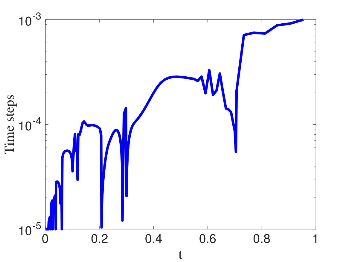 Figure 1
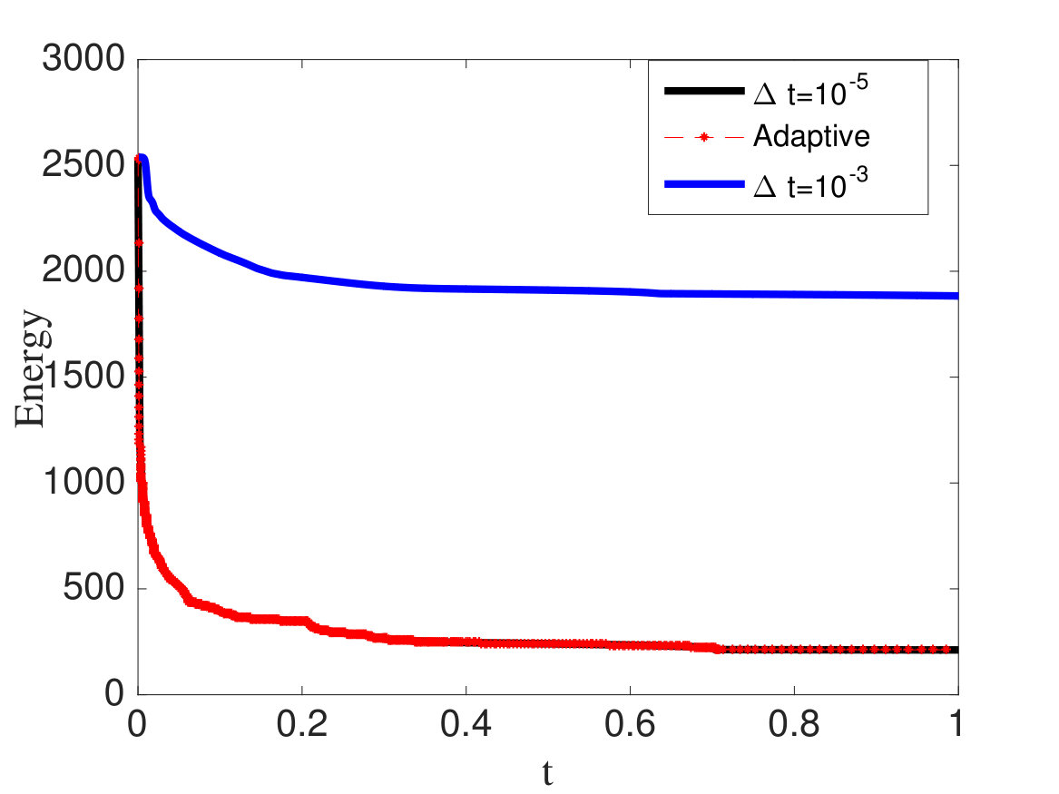 Figure 2
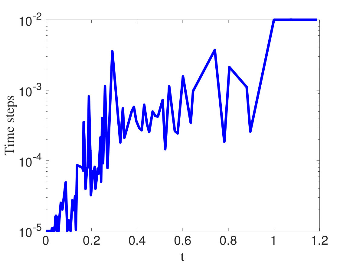 Figure 3
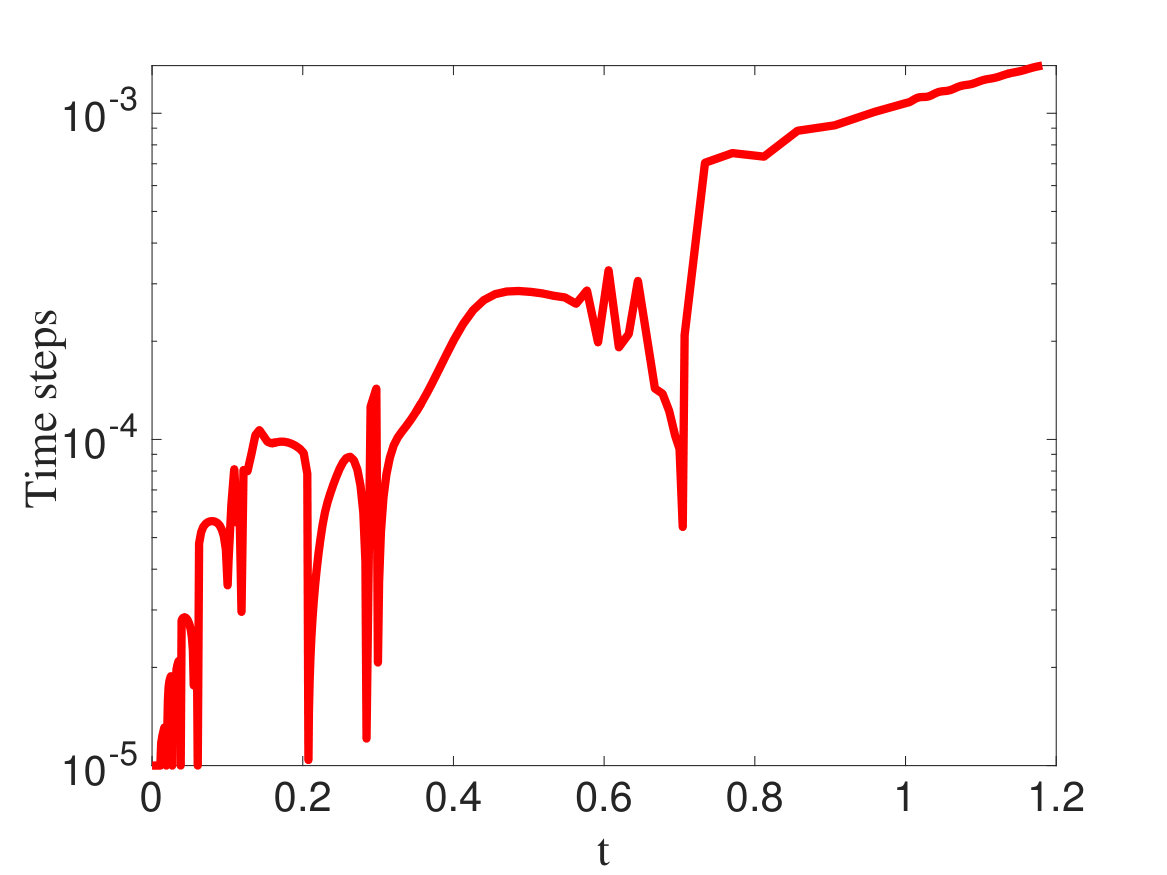 Figure 4
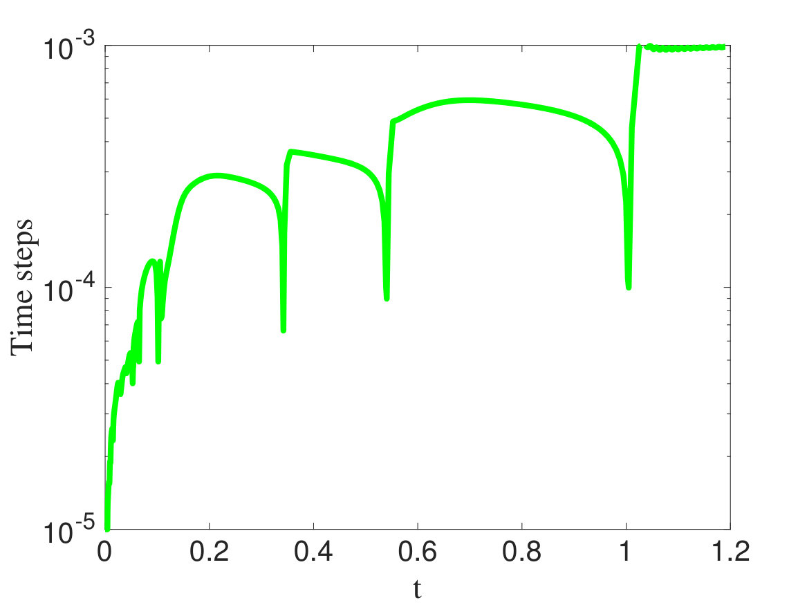 Figure 5
 Figure 1
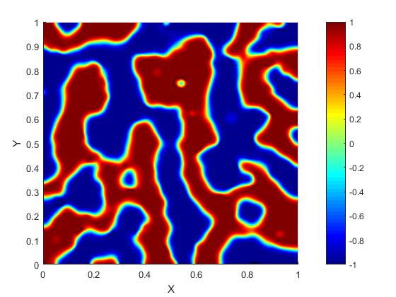 Figure 1
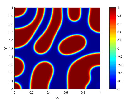 Figure 1
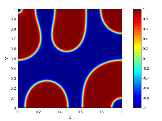 Figure 2
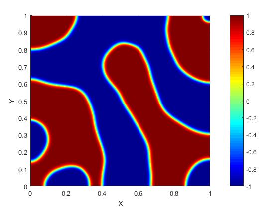 Figure 2
 Figure 2
 Figure 3
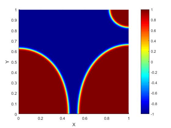 Figure 3
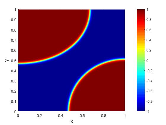 Figure 3
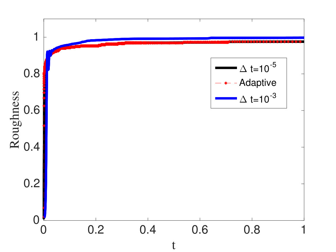 Figure 15
| Rate | Rate | Rate | ||||
|---|---|---|---|---|---|---|
| 6.36E-3 | — | 5.96E-2 | — | 5.93E-3 | — | |
| 1.59E-3 | 2.00 | 1.57E-2 | 1.93 | 1.47E-3 | 2.01 | |
| 3.98E-4 | 2.00 | 3.98E-3 | 1.98 | 3.69E-4 | 2.00 | |
| 9.96E-5 | 2.00 | 9.98E-4 | 1.99 | 9.23E-5 | 2.00 |
| Rate | Rate | Rate | ||||
|---|---|---|---|---|---|---|
| 5.49E-3 | — | 2.78E-2 | — | 4.88E-3 | — | |
| 1.36E-3 | 2.01 | 6.91E-3 | 2.01 | 1.20E-3 | 2.02 | |
| 3.41E-4 | 2.00 | 1.73E-3 | 2.00 | 3.00E-4 | 2.00 | |
| 8.51E-5 | 2.00 | 4.31E-4 | 2.00 | 7.49E-5 | 2.00 |
| Rate | Rate | |||
|---|---|---|---|---|
| 2.50E-2 | — | 2.18E-1 | — | |
| 6.11E-3 | 2.03 | 5.46E-2 | 2.00 | |
| 1.52E-3 | 2.01 | 1.37E-2 | 2.00 | |
| 3.79E-4 | 2.00 | 3.42E-3 | 2.00 |
Peer Reviews
No public reviews on file for this paper yet. If you reviewed it on a platform where reviews are public (OpenReview, ICLR, NeurIPS, ICML), you can paste yours below so the community can read it here.
Videos
No videos yet. Explain this paper in a talk, walkthrough, or lecture? Add one.
Taxonomy
TopicsSolidification and crystal growth phenomena · Advanced Numerical Methods in Computational Mathematics · Fluid Dynamics and Thin Films
\allowdisplaybreaks\nolinenumbers\headers
Energy Stability and Convergence
\externaldocumentex_supplement
Energy Stability and Convergence of SAV
Block-centered Finite Difference Method for Gradient Flows††thanks: Received by editors March 2, 2018
Xiaoli Li School of Mathematics, Shandong University, Jinan 250100, China. Email: [email protected].
Jie Shen Corresponding Author. Department of Mathematics, Purdue University, West Lafayette, IN 47907, USA. Email: [email protected].
Hongxing Rui School of Mathematics, Shandong University, Jinan 250100, China. Email: [email protected].
Abstract
We present in this paper construction and analysis of a block-centered finite difference method for the spatial discretization of the scalar auxiliary variable Crank-Nicolson scheme (SAV/CN-BCFD) for gradient flows, and show rigorously that scheme is second-order in both time and space in various discrete norms. When equipped with an adaptive time strategy, the SAV/CN-BCFD scheme is accurate and extremely efficient. Numerical experiments on typical Allen-Cahn and Cahn-Hilliard equations are presented to verify our theoretical results and to show the robustness and accuracy of the SAV/CN-BCFD scheme.
keywords:
scalar auxiliary variable (SAV), gradient flows, energy stability, block-centered finite difference, error estimates, adaptive time stepping
{AMS}
65M06, 65M12, 65M15, 35K20, 35K35, 65Z05
1 Introduction
Gradient flows are widely used in mathematical models for problems in many fields of science and engineering, particularly in materials science and fluid dynamics, cf. [1, 2, 31, 21] and the references therein. Therefore it is important to develop efficient and accurate numerical schemes for their simulation. There exists an extensive literature on the numerical analysis of gradient flows, see for instance [3, 14, 7, 10, 23, 9, 15] and the references therein.
In the algorithm design of gradient flows, an important goal is to guarantee the energy stability at the discrete level, in order to capture the correct long-time dynamics of the system and provide enough flexibility for dealing with the stiffness problem induced by the thin interface. Many schemes for gradient flows are based on the traditional fully-implicit or explicit discretization for the nonlinear term, which may suffer from harsh time step constraint due to the thin interfacial width [11, 22]. In order to deal with this problem, the convex splitting approach [18, 24, 16] and linear stabilization approach [17, 22, 28, 33] have been widely used to construct unconditionally energy stable schemes. However, the convex splitting approach usually leads to nonlinear schemes and linear stabilization approach is usually limited to first-order accuracy.
Recently, a novel numerical method, the so called invariant energy quadratization (IEQ), was proposed in [29, 32, 30]. This method is a generalization of the method of Lagrange multipliers or of auxiliary variable. The IEQ approach is remarkable as it permits us to construct linear, unconditionally stable, and second-order unconditionally energy stable schemes for a large class of gradient flows. However, it leads to coupled systems with variable coefficients that may be difficult or expensive to solve. The scalar auxiliary variable (SAV) approach [21, 20] was inspired by the IEQ approach, which inherits its main advantages but overcomes many of its shortcomings. In particular, in a recent paper [19], the authors established the first-order convergence and error estimates for the semi-discrete SAV scheme.
In this paper, we construct a SAV/CN scheme with block-centered finite differences for gradient flows, carried out a rigorous stability and error analysis, and implemented an adaptive time stepping strategy so that the time step is only dictated by accuracy rather than by stability. The block-centered finite difference method can be thought as the lowest order Raviart-Thomas mixed element method with a suitable quadrature. Its main advantage over using a regular finite difference method is that it can approximate both the phase function and chemical potential with Neumann boundary conditions in the mixed formulation to second-order accuracy, and it guarantees local mass conservation. Our approach for error estimates here is very different from that in [19] which is based on deriving bounds for the numerical solution. However, this approach can not be used in the fully discrete case with finite-differences in space. The essential tools used in the proof are the summation-by-parts formulae both in space and time to derive energy stability, and an induction process to show that the discrete norm of the numerical solution is uniformly bounded, without assuming a uniform Lipschitz condition on the nonlinear potential. To the best of the authors’ knowledge, this is the first paper with rigorous proof of second-order convergence both in time and space for a linear scheme to a class of gradient flows without assuming a uniform Lipschitz condition for the nonlinear potential.
The paper is organized as follows. In Section 2, we describe our numerical scheme, including the temporal discretization and spacial discretization. In Section 3, we demonstrate the energy stability for our SAV/CN-BCFD scheme. In Section 4, we carry out error estimates for the SAV/CN-BCFD schemes. In Section 5, we present some numerical experiments to verify the energy stability and accuracy of the proposed schemes.
Throughout the paper we use , with or without subscript, to denote a positive constant, which could have different values at different places.
2 The SAV/CN-BCFD scheme
Given a typical energy functional [19]:
[TABLE]
where is a rectangular domain in , and for some , i.e., it is bounded from below. We consider the following gradient flow:
[TABLE]
, and denotes the final time. is the mobility constant which is positive. The chemical potential . for the gradient flow and for the gradient flow. is the nonlinear free energy density and we focus on as an example, when , the and gradient flows are the well-known Allen-Cahn and Cahn-Hilliard equations, respectively.
The boundary and initial conditions are as follows.
[TABLE]
where n is the unit outward normal vector of the domain . The equation satisfies the following energy dissipation law:
[TABLE]
2.1 The semi discrete SAV/CN scheme
We recall the SAV/CN scheme introduced in [21] first.
Let so that . Without loss of generality, we substitute with without changing the gradient flow. Then has a positive lower bound , which we still denote as for simplicity.
In the SAV approach, a scalar variable is introduced, and the system (2.2) can be transformed into:
[TABLE]
Then, the SAV/CN scheme is given as follows:
[TABLE]
where , , can be any explicit approximation of with an error of . For instance, we may let be the extrapolation by
[TABLE]
2.2 Spacial discretization
we apply the BCFD method on the staggered grids for the spacial discretization.
First we give some preliminaries. Let be the standard Banach space with norm
[TABLE]
For simplicity, let
[TABLE]
denote the inner product, And be the standard Sobolev space
[TABLE]
where
[TABLE]
The grid points are denoted by
[TABLE]
and the notations similar to those in [26] are used.
[TABLE]
where and are grid spacings in and directions, and and are the number of grids along the and coordinates, respectively.
Let denote Define the discrete inner products and norms as follows,
[TABLE]
For simplicity, from now on we always omit the superscript (the time level) if the omission does not cause conflicts. Define
[TABLE]
The following discrete-integration-by-part lemma [26] plays an important role in the analysis.
Lemma 2.1**.**
Let be any values such that , then
[TABLE]
[TABLE]
2.2.1 SAV/CV-BCFD scheme for gradient flow
Let us denote by the BCFD approximations to . The scheme for gradient flow is as follows: for ,
[TABLE]
where is an approximation of , and
[TABLE]
The boundary and initial approximations as follows.
[TABLE]
Remark. The solution procedure of the above scheme is described in detail in [21, 20], and hence is omitted here.
2.2.2 SAV/CV-BCFD scheme for gradient flow
Let us denote by the BCFD approximations to . The scheme for gradient flow is as follows: for ,
[TABLE]
where is an approximation of . The boundary and initial conditions are given in (2.16).
3 Unconditional energy stability
We demonstrate below that the full discrete SAV/CN-BCFD schemes are unconditionally energy stable with the discrete energy functional
[TABLE]
where .
3.1 gradient flow
Theorem 3.1**.**
The scheme (2.13)-(2.15) is unconditionally stable and the following discrete energy law holds for any :
[TABLE]
Proof 3.2**.**
Multiplying equation (2.13) by , and making summation on for , we have
[TABLE]
Using Lemma 2.1, equation (3.3) can be transformed into the following:
[TABLE]
Multiplying equation (2.14) by , and making summation on for , we have
[TABLE]
Using Lemma 2.1 again, the first term on the right hand side of equation (3.5) can be written as:
[TABLE]
Multiplying equation (2.15) by leads to
[TABLE]
Combining equation (3.7) with equations (3.4) - (3.6) gives that
[TABLE]
which implies the desired results (3.2).
3.2 gradient flow
For gradient flow, we shall only state the result, as its proof is essentially the same as for the gradient flow.
Theorem 3.3**.**
The scheme (2.17)-(2.19) is unconditionally stable and the following discrete energy law holds for any :
[TABLE]
4 Error estimates
In this section, we derive our main results of this paper, i.e., error estimates for the fully discrete SAV/CN-BCFD schemes.
For simplicity, we set
[TABLE]
4.1 gradient flow
We shall first derive error estimates for the case of gradient flow.
Theorem 4.1**.**
We assume that and . Let , then for the discrete scheme (2.13)-(2.15), there exists a positive constant independent of , and such that
[TABLE]
We shall split the proof of the above results into three lemmas below.
Lemma 4.2**.**
Under the condition of Theorem 4.1, there exists a positive constant independent of , and such that
[TABLE]
Proof 4.3**.**
Denote
[TABLE]
Subtracting equation (2.5) from equation (2.13), we obtain
[TABLE]
where
[TABLE]
[TABLE]
Subtracting equation (2.6) from equation (2.14) leads to
[TABLE]
where
[TABLE]
Subtracting equation (2.7) from equation (2.15) gives that
[TABLE]
where
[TABLE]
Multiplying equation (4.3) by , and making summation on for , we have
[TABLE]
Using Lemma 2.1, we can write the first term on the right hand side of equation (4.10) as:
[TABLE]
Thanks to Cauchy-Schwarz inequality, the last two terms on the right hand side of equation (4.11) can be transformed into:
[TABLE]
Multiplying equation (4.6) by , and making summation on for , we have
[TABLE]
Similar to the estimate of equation (3.6), the first term on the right hand side of equation (4.13) can be transformed into the following:
[TABLE]
The second term on the right hand side of equation (4.13) can be rewritten as follows:
[TABLE]
Recalling equation (4.3), the first term on the right hand side of equation (4.15) can be transformed into the following:
[TABLE]
Next, we shall first make the hypothesis that there exists a positive constant such that
[TABLE]
This hypothesis will be verified in Lemma 4.6 using a bootstrap argument.
Since , we have
[TABLE]
Using above and the Cauchy-Schwartz inequality, we can deduce that
[TABLE]
Similarly we can obtain
[TABLE]
Then equation (4.16) can be estimated by:
[TABLE]
Similar to (4.16), the second term on the right hand side of equation (4.15) can be controlled by:
[TABLE]
The third term on the right hand side of equation (4.13) can be estimated by:
[TABLE]
Multiplying equation (4.8) by leads to
[TABLE]
The first and second terms on the right hand side of equation (4.24) can be transformed into:
[TABLE]
Since , we have that
[TABLE]
*Recalling the midpoint approximation property of the rectangle quadrature formula, we can obtain that *
[TABLE]
*Combining equation (4.24) with equations (4.10)-(4.27) and using Cauchy-Schwarz inequality result in *
[TABLE]
From the discrete-integration-by-parts,
[TABLE]
we find
[TABLE]
Similarly we have
[TABLE]
Multiplying equation (4.29) by , summing over and combining with equations (4.31) and (4.32), we can obtain (4.2).
Lemma 4.4**.**
Under the condition of Theorem 4.1, there exists a positive constant independent of , and such that
[TABLE]
Proof 4.5**.**
Multiplying equation (4.3) by , and making summation on for , we have
[TABLE]
Using Lemma 2.1, the first term on the right hand side of equation (4.34) can be transformed into the following:
[TABLE]
The first term on the right hand side of equation (4.35) can be estimated as:
[TABLE]
In the direction, we have the similar estimates. Then the left hand side in (4.35) can be bounded by:
[TABLE]
Thanks to (4.6) and (4.15), the first term on the right hand side of (4.37) can be estimated as follows:
[TABLE]
Combining equation (4.34) with equations (4.37) and (4.38) and multiplying equation (4.29) by , summing over lead to (4.33).
Lemma 4.6**.**
Under the condition of Theorem 4.1, there exists a positive constant independent of , and such that
[TABLE]
Proof 4.7**.**
We proceed in two steps.
Step 1 (Definition of ): Using the scheme (2.13)-(2.15) for and applying the inverse assumption, we can get the approximation with the following property:
[TABLE]
where and is an bilinear interpolant operator with the following estimate [6]:
[TABLE]
Thus we can choose the positive constant independent of and such that
[TABLE]
Step 2 (Induction): By the definition of , it is trivial that hypothesis (4.17) holds true for . Supposing that holds true for an integer , with the aid of the estimate (4.42), we have that
[TABLE]
Next we prove that holds true. Since
[TABLE]
Let and a positive constant be small enough to satisfy
[TABLE]
Then for we derive from (4.40) that
[TABLE]
This completes the induction.
We are now in position to prove our main results.
Proof 4.8** (Proof of Theorem 4).**
Thanks to the above three lemmas, we can obtain
[TABLE]
Finally applying the discrete Gronwall’s inequality, we arrive at the desired result:
[TABLE]
Thus, the proof of Theorem 4 is complete.
4.2 gradient flow
For the gradient flow, we shall only state the error estimates below, as their proofs are essentially the same as for the gradient flow.
Theorem 4.9**.**
We assume that and and . Then for the discrete scheme (2.17)-(2.19), there exists a positive constant independent of , and such that
[TABLE]
5 Numerical simulations
We present in this section various numerical experiments to verify the energy stability and accuracy of the proposed numerical schemes.
5.1 Accuracy test for Allen-Cahn and Cahn-Hilliard equations
We consider the free energy
[TABLE]
and for better accuracy, rewrite it as
[TABLE]
where is a positive number to be chosen. To apply our schemes (2.13)-(2.15) or (2.17)-(2.19) to the system (2.2), we drop the constant in the free energy and specify the operator , the energy and as follows:
[TABLE]
The system (2.2) becomes the standard Allen-Cahn equation with , and the standard Cahn-Hilliard equation with .
We denote
[TABLE]
where and .
In the following simulations, we choose and .
5.1.1 Convergence rates of the SAV/CN-BCFD scheme for Allen-Cahn equation
Example 1. We take , and the initial solution . To get around the fact that we do not have possession of exact solution, we measure Cauchy error, which is similar to [5, 27, 7]. Specifically, the error between two different grid spacings and is calculated by .
The numerical results are listed in Table 1. we observe the second-order convergence predicted by the error estimates in Theorem 4.9.
5.1.2 Convergence rates of SAV/CN-BCFD scheme for Cahn-Hilliard equation
Example 2. We take , with the same initial solution as in Example 1. The numerical results are listed in Tables 2 and 3. Again, we observe the expected second-order convergence rate in various discrete norms.
5.2 Coarsening dynamics and adaptive time stepping
In this example, we simulate the coarsening dynamics of the Cahn-Hilliard equation.
Since the scheme (2.13)-(2.15) is unconditionally energy stable, we can choose time steps according to accuracy only with an adaptive time stepping. Actually in many situations, the energy and solution of gradient flows can vary drastically in certain time intervals, but only slightly elsewhere. In order to maintain the desired accuracy, we adjust the time sizes based on an adaptive time-stepping strategy below (Ref. [13, 20]).
We update the time step size by using the formula
[TABLE]
where is a default safety coefficient, is a reference tolerance, and is the relative error at each time level. In this simulation, we take
[TABLE]
with a random initial condition with values in , and the initial time step is taken as .
To demonstrate the effectivity of the SAC/CN-BCFD scheme with adaptive time stepping, we compute the reference solutions with a small uniform time step and a large uniform time step respectively. Characteristic evolutions of the phase functions are presented in Fig. 1(c). We also present in Fig. 2 the energy evolutions and the roughness of interface, where the roughness measure function is defined as follows:
[TABLE]
with . One observes that the solution obtained with adaptive time steps is consistent with the reference solution obtained with a small time step, while the solution with large time step deviates from the reference solution. This is also verified by both the energy evolutions and roughness measure function . We present in Fig. 3 the adaptive time steps for different . We observe that there are about two-orders of magnitude variation in the time steps with the adaptive time stepping, which indicates that the adaptive time stepping for the SAV/CN-BCFD scheme is very efficient.
Acknowledgments
X. Li thanks for the financial support from China Scholarship Council. The work of J. Shen is supported in part by NSF grants DMS-1620262, DMS-1720442 and AFOSR grant FA9550-16-1-0102. The work of H. Rui is supported by the National Natural Science Foundation of China grant 11671233.
The reference list from the paper itself. Each links out to its DOI / PubMed record.
- 1[1] J. W. Cahn and J. E. Hilliard , Free energy of a nonuniform system. I 𝐼 I . Interfacial free energy , The Journal of chemical physics, 28 (1958), pp. 258–267.
- 2[2] J. W. Cahn and J. E. Hilliard , Free energy of a nonuniform system. I I I 𝐼 𝐼 𝐼 III . nucleation in a two-component incompressible fluid , The Journal of chemical physics, 31 (1959), pp. 688–699.
- 3[3] W. Chen, Y. Liu, C. Wang, and S. Wise , Convergence analysis of a fully discrete finite difference scheme for the Cahn-Hilliard-Hele-Shaw equation , Mathematics of Computation, 85 (2015), pp. 2231–2257.
- 4[4] X. Chen, C. M. Elliott, A. Gardiner, and J. J. Zhao , Convergence of numerical solutions to the Allen-Cahn equation , Applicable Analysis, 69 (1998), pp. 47–56.
- 5[5] Y. Chen and J. Shen , Efficient, adaptive energy stable schemes for the incompressible Cahn-Hilliard Navier-Stokes phase-field models , Journal of Computational Physics, 308 (2016), pp. 40–56.
- 6[6] C. N. Dawson, M. F. Wheeler, and C. S. Woodward , A two-grid finite difference scheme for nonlinear parabolic equations , SIAM journal on numerical analysis, 35 (1998), pp. 435–452.
- 7[7] A. E. Diegel, X. H. Feng, and S. M. Wise , Analysis of a mixed finite element method for a Cahn-Hilliard-Darcy-Stokes system , SIAM Journal on Numerical Analysis, 53 (2015), pp. 127–152.
- 8[8] A. E. Diegel, C. Wang, and S. M. Wise , Stability and convergence of a second-order mixed finite element method for the cahn?hilliard equation , Ima Journal of Numerical Analysis, 36 (2015), pp. 1867–1891.