Graphical Models for Extremes
Sebastian Engelke, Adrien S. Hitz

TL;DR
This paper develops a new graphical model framework for multivariate extreme value distributions, enabling sparse and interpretable models for high-dimensional rare event data, with applications to flood risk assessment.
Contribution
It introduces a general theory of conditional independence for multivariate Pareto distributions, linking it to graphical models and sparsity in extreme value analysis.
Findings
Hammersley-Clifford theorem for extremal graphical models
Sparsity patterns can be inferred from inverse covariance matrices
Application to flood risk assessment on the Danube river
Abstract
Conditional independence, graphical models and sparsity are key notions for parsimonious statistical models and for understanding the structural relationships in the data. The theory of multivariate and spatial extremes describes the risk of rare events through asymptotically justified limit models such as max-stable and multivariate Pareto distributions. Statistical modelling in this field has been limited to moderate dimensions so far, partly owing to complicated likelihoods and a lack of understanding of the underlying probabilistic structures. We introduce a general theory of conditional independence for multivariate Pareto distributions that allows the definition of graphical models and sparsity for extremes. A Hammersley-Clifford theorem links this new notion to the factorization of densities of extreme value models on graphs. For the popular class of H\"usler-Reiss distributions…
Click any figure to enlarge with its caption.
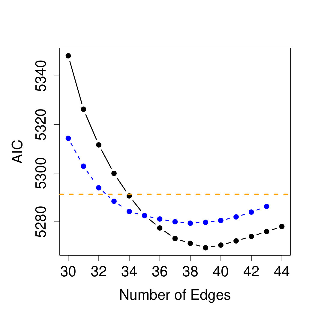 Figure 1
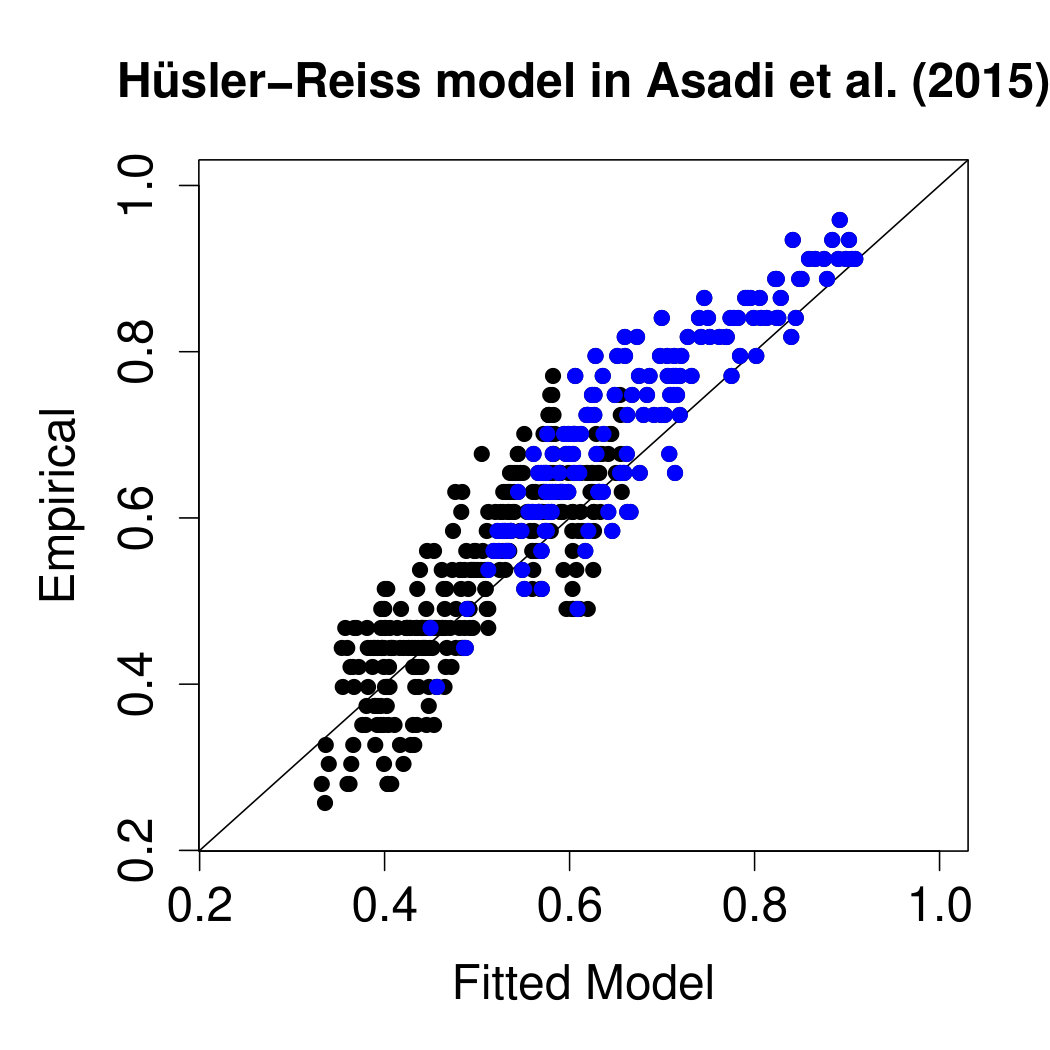 Figure 2
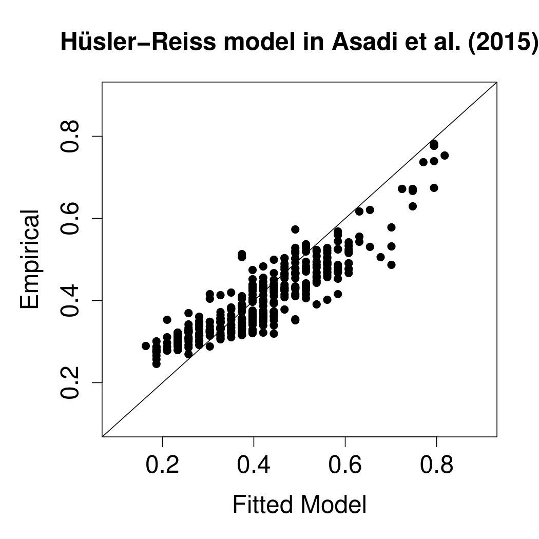 Figure 3
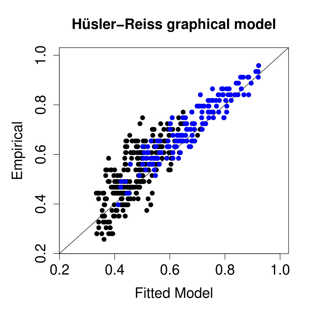 Figure 4
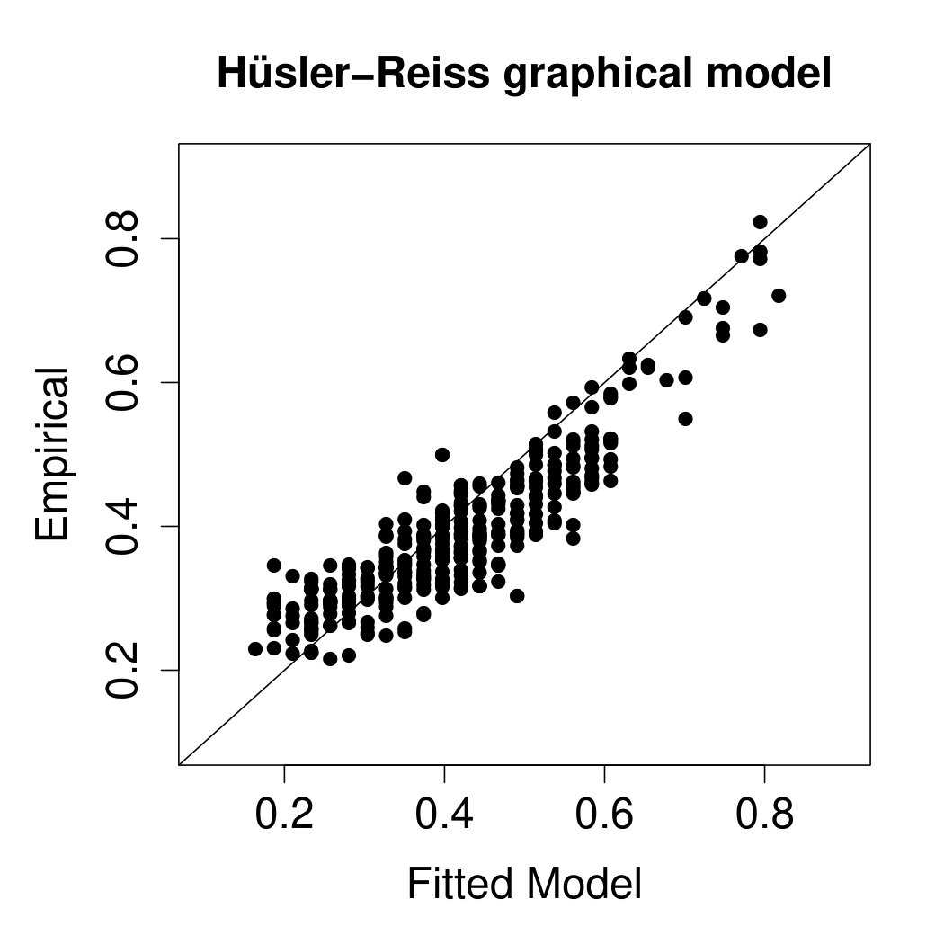 Figure 5
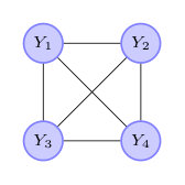 Figure 6
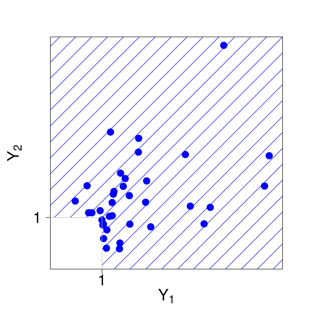 Figure 7
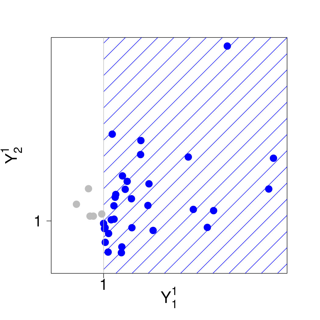 Figure 8
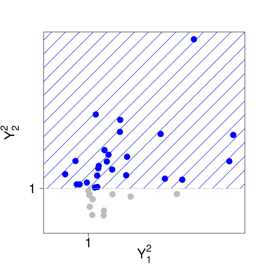 Figure 9
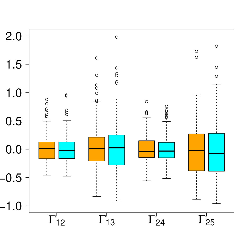 Figure 10
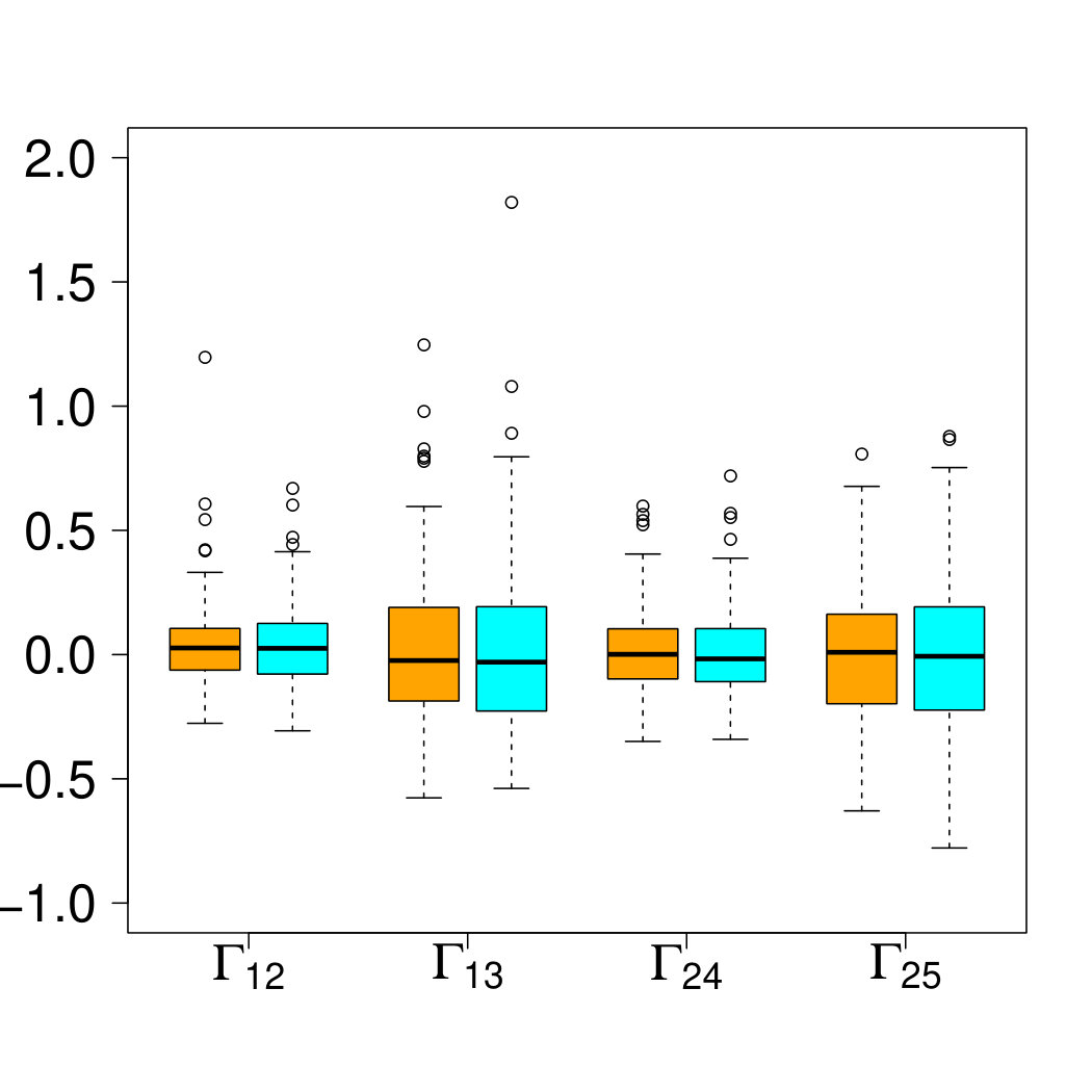 Figure 11
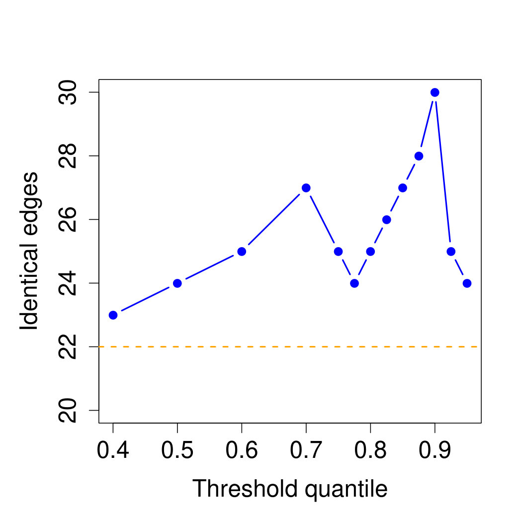 Figure 12
Peer Reviews
No public reviews on file for this paper yet. If you reviewed it on a platform where reviews are public (OpenReview, ICLR, NeurIPS, ICML), you can paste yours below so the community can read it here.
Videos
No videos yet. Explain this paper in a talk, walkthrough, or lecture? Add one.
Graphical Models for Extremes
Sebastian Engelke
Research Center for Statistics, University of Geneva, Boulevard du Pont d’Arve 40, 1205 Geneva, Switzerland.
Adrien S. Hitz
Department of Statistics, University of Oxford, 24-29 St Giles’, Oxford OX1 3LB, UK and Materialize.X, Enterprise Lab, Imperial College London, London SW7 2AZ, UK.
Abstract
Conditional independence, graphical models and sparsity are key notions for parsimonious statistical models and for understanding the structural relationships in the data. The theory of multivariate and spatial extremes describes the risk of rare events through asymptotically justified limit models such as max-stable and multivariate Pareto distributions. Statistical modelling in this field has been limited to moderate dimensions so far, partly owing to complicated likelihoods and a lack of understanding of the underlying probabilistic structures. We introduce a general theory of conditional independence for multivariate Pareto distributions that allows the definition of graphical models and sparsity for extremes. A Hammersley–Clifford theorem links this new notion to the factorization of densities of extreme value models on graphs. For the popular class of Hüsler–Reiss distributions we show that, similarly to the Gaussian case, the sparsity pattern of a general extremal graphical model can be read off from suitable inverse covariance matrices. New parametric models can be built in a modular way and statistical inference can be simplified to lower-dimensional marginals. We discuss learning of minimum spanning trees and model selection for extremal graph structures, and illustrate their use with an application to flood risk assessment on the Danube river.
Keywords: Extreme value theory; Conditional independence; Multivariate Pareto distribution; Graphical models; Sparsity
1 Introduction
Evaluation of the risk related to heat waves, extreme flooding, financial crises, or other rare events requires the quantification of their small occurrence probabilities. Empirical estimates are unreliable since the regions of interest are in the tail of the distribution and typically contain few or no data points. Extreme value theory provides the theoretical foundation for extrapolations to the distributional tail of a -dimensional random vector . The univariate case is well-studied and the generalized extreme value and Pareto distributions are widely applied in areas such as hydrology (Katz et al., 2002), climate science (Min et al., 2011) and finance (McNeil et al., 2015); see also Embrechts et al. (1997) and Beirlant et al. (2004).
In the multivariate setting, , the result of the extrapolation strongly depends on the strength of extremal dependence between the components of . Most current statistical models assume multivariate regular variation for (Resnick, 2008) since this entails mathematically elegant descriptions of the asymptotic tail distribution. Similar to the univariate setting, two different but closely related approaches exist. Max-stable distributions arise as limits of normalised maxima of independent copies of and have been extensively studied and applied in multivariate and spatial risk problems (cf., de Haan, 1984; Gudendorf and Segers, 2010; Davison et al., 2012). On the other hand, multivariate Pareto distributions describe the random vector conditioned on the event that at least one component exceeds a high threshold; see Rootzén and Tajvidi (2006), Rootzén et al. (2018) and Kiriliouk et al. (2018) for their construction, stability properties and statistical inference.
A drawback of the current multivariate models is their limitation to rather moderate dimensions , and the construction of tractable parametric models in higher dimensions is challenging, both for max-stable and multivariate Pareto distributions. Sparse multivariate models require the notion of conditional independence (Dawid, 1979), which is not easy to define for tail distributions. In fact, Papastathopoulos and Strokorb (2016) show that if is a max-stable random vector with positive continuous density, then the conditional independence of already implies the independence ; see also Dombry and Éyi-Minko (2014). Meaningful conditional independence structures can thus only be obtained for max-stable distributions with discrete spectral measure (Gissibl and Klüppelberg, 2018). Since these models do not admit densities, this excludes most of the currently used parametric families.
In this work we take the perspective of threshold exceedances and introduce a new notion of conditional independence for a multivariate Pareto distribution , which we denote by to stress that it is designed for extremes. It is different from classical conditional independence since the support of is not a product space, but the homogeneity property of can be used to show that it is well-defined. Conditional independence is tightly linked to graphical models. For an undirected graph with nodes and edge set , we say that is an extremal graphical model if it satisfies the pairwise Markov property
[TABLE]
The main advantage of conditional independence and graphical models is that they imply a simple probabilistic structure and possibly sparse patterns in multivariate random vectors (Lauritzen, 1996; Wainwright and Jordan, 2008). For extremal graphical models on decomposable graphs, we prove a Hammersley–Clifford type theorem stating that (1) is equivalent to the factorization of the density of into lower-dimensional marginals. This underlines that our notion of conditional independence is in fact natural for multivariate Pareto distributions.
Applications of this result are manifold. From a probabilistic perspective, we analyse models in the literature regarding their graphical properties in the sense of our definition (1). Extremal graphical models whose underlying graph is a tree have a particularly simple multiplicative stochastic representation in terms of extremal functions, a notion that is known from the simulation of max-stable processes (Dombry et al., 2016). In multivariate extremes, one may argue that the family of Hüsler–Reiss distributions (Hüsler and Reiss, 1989) takes a similar role as Gaussian distributions in the non-extreme world. Instead of covariance matrices, they are parameterized by a variogram matrix . We show that the extremal graphical structure of a Hüsler–Reiss distribution can be identified by zero patterns on matrices derived from .
Extremal graphical models enable the construction of parsimonious models for multivariate Pareto distributions , which further enjoy the advantage of interpretability in terms of the underlying graph. Thanks to the factorization of the densities, statistical inference can be efficiently carried out on lower-dimensional marginals. For decomposable graphs with singleton separator sets, so-called block graphs, this allows the use of multivariate Pareto models in fairly high dimensions. In many cases the underlying graphical structure is unknown and has to be learned from data. We discuss how a maximum likelihood tree can be obtained using standard algorithms by Kruskal (1956) or Prim (1957), and how the best model can be selected among different extremal graphical models.
There is previous work on the construction of parsimonious extreme value models. A large body of literature studies spatial max-stable random fields (Schlather, 2002; Kabluchko et al., 2009; Opitz, 2013). Such models have small parameter dimension but they rely on strong assumptions on stationarity and cannot be applied to multivariate, non-spatial data without information on an underlying space. Other approaches include constructions through factor copulas (Lee and Joe, 2018), ensembles of trees combining bivariate copulas (Yu et al., 2017), graphical models for large censored observations (Hitz and Evans, 2016) and eigendecompositions (Cooley and Thibaud, 2018). Closely related to our concept of conditional independence is the work of Coles and Tawn (1991) and Smith et al. (1997) who propose a Markov chain model where all bivariate marginals are extreme value distributions. This can be seen as a special case of our approach when the graph has the simple structure of a chain. Similar limiting objects also arise as the tail chains in the theory of extremes of stationary Markov chains with regularly varying marginals (Smith, 1992; Basrak and Segers, 2009; Janssen and Segers, 2014). This theory has recently been extended to regularly varying Markov trees (Segers, 2019). Gissibl and Klüppelberg (2018) and Gissibl et al. (2018) study the causal structure of directed acyclic graphs for max-linear models, and they develop methods for model identification based on tail dependence coefficients. Their work is in some sense complementary to ours, since their models do not possess densities whereas we will explicitly assume the existence of densities.
To the best of our knowledge, our work is the first principled attempt to define conditional independence for general multivariate extreme value models that naturally extends to the factorization of densities, sparsity and graphical models. Section 2 introduces background on extreme value theory and graphical models needed throughout the paper. The new notion of conditional independence is defined in Section 3 and equivalent properties are derived. Section 4 contains the main probabilistic results on extremal graphical models, the representation of trees and the characterization for Hüsler–Reiss distributions. Statistical models on block graphs and their estimation, simulation and model selection are discussed in Section 5. In these graphical models the dependence is modeled directly between lower-dimensional subsets of variables, whereas the global dependence is implicitly implied by the conditional independence structure of the graph. There are many potential applications of extremal graphical models. In Section 6, we illustrate the advantages of this structured approach compared to classical extreme value models on a data set related to flooding on a river network in the upper Danube basin (cf., Asadi et al., 2015). The interpretation of the graphical structures obtained in this application is particularly interesting since there is a seemingly natural underlying tree associated to the flow-connections. Our conditional independence is formulated for multivariate Pareto distributions, but the results in this paper have implications for max-stable distributions. This point and further research directions will be addressed in the discussion in Section 7. The Appendix contains proofs and some additional results.
An implementation for R (R Core Team, 2019) is available in the package graphicalExtremes (Engelke et al., 2019). The code for the simulation study and application can be found in the supplementary material.
2 Background
2.1 Notation
We introduce some standard notation that is used throughout the paper. Symbols in boldface such as are column vectors with components denoted by , , and operations and relations involving such vectors are meant componentwise. The vectors and are used as generic vectors with suitable dimension. Denoting the index set by , for a non-empty subset , we write for the subvectors and . Similar notation is used for random vectors with values in . For a matrix with entries indexed by , and subsets we let denote the submatrix of , and we abbreviate . For with , a multivariate interval is denoted by . The -norm of a vector for is , and its -norm is . The density of a random vector , if it exists, is denoted by . The density of the marginal for a non-empty is denoted by , if there is no ambiguity regarding the random vector.
2.2 Multivariate extreme value theory
The tail behavior of the random vector can be described through two different approaches, one based on componentwise maxima and the other one on threshold exceedances. We briefly discuss both approaches and the close link between them.
Let , , be independent copies of and denote the componentwise maximum by . Under mild conditions on the marginal distribution of there exist sequences of normalizing constants , , , such that
[TABLE]
where , and is the generalized extreme value distribution whose shape parameter determines the heaviness of the tail of ; see de Haan and Ferreira (2006); Embrechts et al. (1997) and Beirlant et al. (2004) for details. For analysis of the dependence structure, the marginal distributions of are typically estimated first to normalise the data by to standard Pareto distributions. For simplicity, we assume in the sequel that the are known and the vector has been normalised to standard Pareto marginals. Joint estimation of marginals and dependence is discussed in Section 5.2.
The standardized vector is said to be in the max-domain of attraction of the random vector if for any
[TABLE]
In this case, is max-stable with standard Fréchet marginals , , and we may write
[TABLE]
where the exponent measure is a Radon measure on the cone , and is shorthand for . If is absolutely continuous with respect to Lebesgue measure on , its Radon–Nikodym derivative, denoted by , has the following properties:
- (L1)
homogeneity of order , i.e., for any and ;
- (L2)
normalised marginals, i.e., for any ,
[TABLE]
The two properties follow from the max-stability and the standard Fréchet marginals of , respectively. For a non-empty subset , we define the marginal of by
[TABLE]
and note that it is homogeneous of order . In particular, if for some , then as a consequence of (L1) and (L2). Conversely, any positive and continuous function satisfying (L1) and (L2) defines a valid density of an exponent measure by integration over , , that satisfies similar homogeneity and normalization properties as . By (4) this also defines a max-stable distribution.
Another perspective on multivariate extremes is through threshold exceedances. By Proposition 5.17 in Resnick (2008), the convergence in (3) is equivalent to
[TABLE]
Consequently, the multivariate distribution of the threshold exceedances of satisfies
[TABLE]
The distribution of the limiting random vector is called a multivariate Pareto distribution (cf., Rootzén and Tajvidi, 2006). It is defined through the exponent measure of the max-stable distribution , with support on the -shaped space . We say that and are associated, since their distributions mutually determine each other.
Multivariate Pareto distributions are the only possible limits in (6) and, owing to the homogeneity of the exponent measure, they enjoy certain stability properties (cf., Rootzén et al., 2018). The exponent measure , and hence the distribution of , may place mass on some lower-dimensional faces of the space . For the remainder of this paper we exclude this case to avoid technical difficulties. We further assume that the distribution of admits a positive and continuous density on , which is
[TABLE]
since is always constant along at least one coordinate for . The density is thus proportional to the density of the exponent measure . By the homogeneity of , is also homogeneous of order . The normalization constant is known as the -variate extremal coefficient (cf., Schlather and Tawn, 2003). The assumption of a positive and continuous density implies that the multivariate Pareto distributions we study are models for asymptotic extremal dependence, and all -variate extremal coefficients, , are strictly smaller than their upper limit .
For some non-empty subset , the subvector , properly normalised, given that its -norm is large converge in the sense of (6) to the marginal of defined on with homogeneous density of order given by
[TABLE]
where is the exponent measure of , and is the density of .
Example 1** (Logistic distribution).**
The extremal logistic distribution with parameter induces a multivariate Pareto distribution with density
[TABLE]
Example 2** (Hüsler–Reiss distribution).**
The Hüsler–Reiss distribution (Hüsler and Reiss, 1989) is parameterized by a symmetric, strictly conditionally negative definite matrix with and non-negative entries, that is, for all non-zero vectors with . The corresponding density of the exponent measure can be written for any as (cf., Engelke et al., 2015)
[TABLE]
where is the density of a centred -dimensional normal distribution with covariance matrix , and
[TABLE]
The matrix is strictly positive definite; see Appendix B for details. The representation of the density in (9) seems to depend on the choice of , but, in fact, the value of the right-hand side of this equation is independent of . The Hüsler–Reiss multivariate Pareto distribution has density and the strength of dependence between the th and th component is parameterized by , ranging from complete dependence for and independence for . In the bivariate case we have
[TABLE]
and , where is the standard normal distribution function. The extension of Hüsler–Reiss distributions to random fields are Brown–Resnick processes (Brown and Resnick, 1977; Kabluchko et al., 2009), which are widely used models for spatial extremes.
Example 3** (Bivariate Pareto distribution).**
In the general bivariate case , due to homogeneity, the density of the exponent measure can be characterised by a univariate distribution. Indeed, for any positive random variable with density and ,
[TABLE]
satisfies conditions (L1) and (L2) above and thus defines a valid exponent measure density. We call the extremal function at coordinate , relative to coordinate (cf., Dombry et al., 2013, 2016). Equivalently, we can write the density in terms of the extremal function at coordinate , relative to coordinate , as , , and is related to via the measure change , .
The above is a general construction principle, since every valid exponent measure density can be obtained in this way. The bivariate Hüsler–Reiss distribution in (11) corresponds to the case of log-normal and , but many other parametric and non-parametric examples are available (e.g., Boldi and Davison, 2007; Cooley et al., 2010; Ballani and Schlather, 2011; de Carvalho and Davison, 2014).
2.3 Graphical models
A graph is defined as a set of nodes , also called vertices, together with a set of edges of pairs of distinct nodes. The graph is called undirected if for two nodes , if and only if . For notational convenience, for undirected graphs we sometimes represent edges as unordered pairs . When counting the number of edges, we count such that each edge is considered only once. A subset of nodes is called complete if it is fully connected in the sense that for all . We denote by the set of all cliques, that is, the complete subsets that are not properly contained within any other complete subset.
To each node we associate a random variable with continuous state space . The resulting random vector takes values in the Cartesian product . Suppose that has a positive and continuous Lebesgue density on . For three disjoint subsets whose union is , we say that is conditionally independent of given if the density factorizes as
[TABLE]
and we write . If , then (13) amounts to independence of and .
The random vector is said to be a probabilistic graphical model on the graph if its distribution satisfies the pairwise Markov property relative to , that is, for all . If in addition, for any disjoint subsets such that separates from in , , then is said to obey the global Markov property relative to . Since is positive and continuous, it follows from the Hammersley–Clifford theorem (cf., Lauritzen, 1996, Theorem 3.9) that the two Markov properties are equivalent, and they are further equivalent to the factorization of the density
[TABLE]
for suitable functions on . If the graph is decomposable, then this factorization can be rewritten in terms of marginal densities
[TABLE]
where is a multiset containing intersections between the cliques called separator sets; see Lauritzen (1996) and Appendix A for the definition of decomposability and separator sets.
Example 4**.**
We recall that for a normal distribution with invertible covariance matrix , the precision matrix contains the conditional independencies, or equivalently the graph structure, since for ,
[TABLE]
3 Conditional independence for threshold exceedances
The notion of conditional independence has not been exploited in extreme value theory. In fact, for max-stable distributions it only leads to trivial probabilistic structures (Papastathopoulos and Strokorb, 2016). An exception are directed acyclic graphs for max-linear models studied in Gissibl and Klüppelberg (2018) and Gissibl et al. (2018), which do however not admit densities.
We therefore approach the problem from the perspective of threshold exceedances. Since the notion of independence is only defined on product spaces, the meaning of conditional independence is not straightforward for a multivariate Pareto distribution , , with support on the -shaped space . In this section we show that there is nevertheless a natural definition of conditional independence for . To this end, we restrict to product spaces. For any , we consider the random vector defined as conditioned on the event that . Clearly, has support on the product space (cf., Figure 1) and it admits the density
[TABLE]
since because of (L2) in Section 2.2. From (16) we see that the densities coincide with on the intersection of their supports. Therefore there are no problems with lack of self-consistency as for instance in the model of Heffernan and Tawn (2004).
For any set with , the marginal has density
[TABLE]
which is homogeneous of order on ; see (5). This is however not the case if , since integration over then includes whose domain is in , and thus in general ,
Definition 1**.**
Suppose that is multivariate Pareto and admits a positive and continuous density on , and let be non-empty disjoint subsets whose union is . We say that is conditionally independent of given if
[TABLE]
In this case we write .
In fact, this definition can be shown to be equivalent to a slightly weaker condition, and to a factorization of the exponent measure density .
Proposition 1**.**
Let and the sets be as in the above definition, then is equivalent to any of the following two conditions.
- (i)
[TABLE] 2. (ii)
The density of the exponent measure factorizes as
[TABLE]
A natural question is whether one can extend the definition of to the case where , meaning that and are independent on . In terms of the original definition, that would mean that for any , for all . Without losing generality, suppose , then for any and . Therefore would be homogeneous of order and thus not integrable on , a contradiction. In the next section we show that this property implies that all graphical models defined in terms of the conditional independence must be connected.
4 Graphical models for threshold exceedances
The notion of conditional independence allows us to define graphical models for threshold exceedances. As before, let be the positive and continuous density on of a multivariate Pareto distribution , proportional to the density of the exponent measure , and homogeneous of order . Let be an undirected graph with nodes and edge set . Similarly to the classical probabilistic graphical models described in Section 2.3, we say that satisfies the pairwise Markov property on relative to if
[TABLE]
that is, and are conditionally independent in the sense of Definition 1 given all other nodes whenever there is no edge between and in . By definition, this is equivalent to saying that satisfies the usual pairwise Markov property on relative to for all . The global Markov property for is defined similarly.
Definition 2**.**
Let be an undirected graph. If the multivariate Pareto distribution with positive and continuous density satisfies the pairwise Markov property (20) relative to , we call the distribution of an extremal graphical model with respect to .
For a decomposable graph we obtain a factorization of the density similar to the classical Hammersley–Clifford theorem, showing that the Definition 1 of conditional independence is natural for multivariate Pareto distributions. Let and be the sequences of cliques and separators of , respectively, satisfying the running intersection property (44) in Appendix A.
Theorem 1**.**
Let be a decomposable graph and suppose that has a multivariate Pareto distribution with positive and continuous density on . Denote the corresponding exponent measure and its density by and , respectively. Then the following are equivalent.
- (i)
The distribution of satisfies the pairwise Markov property relative to 2. (ii)
The distribution of satisfies the global Markov property relative to 3. (iii)
The density factorizes according to , that is,
[TABLE]
where the marginals are positive, continuous and homogeneous of order for any .
In all cases, the graph is necessarily connected.
Remark 1**.**
The above theorem shows that only connected extremal graphical models can arise. This is related to the assumption of multivariate regular variation in (3) that implies asymptotic dependence between all components. Loosely speaking, unconnected components would correspond to asymptotically independent components.
Remark 2**.**
If the graph in the above theorem is non-decomposable, it is expected that the density still factorizes into factors on the cliques of the graph. These factors can however no longer be identified with marginal densities, and it is an open problem whether they can be chosen to be homogeneous.
Since is not a product space, unlike in the classical Hammersley–Clifford theorem for decomposable graphs in (15), the factors in the factorization of the density in (21) are not the marginals but the marginals of the exponent measure density . It holds however that for all .
As a first application, the above theorem allows us to formally analyse the conditional independencies and graphical structures of models in the multivariate extreme value literature.
Example 5**.**
One of the simplest examples of a graph is a chain, that is,
[TABLE]
Coles and Tawn (1991)** proposed a model that factorizes with respect to this chain where all bivariate marginals are logistic (cf., Example 1). This was extended to general bivariate marginals in Smith et al. (1997). More generally, in the study of extremes of stationary Markov chains the limiting objects are so-called tail chains. The latter induce multivariate Pareto distributions that can readily be seen to factorize with respect to a chain; see Smith (1992) Basrak and Segers (2009) and Janssen and Segers (2014).
Example 6**.**
It turns out that many of the multivariate models in the literature do not have any conditional independencies, that is, their underlying graph is fully connected. For instance, this holds for the logistic multivariate Pareto distribution in Example 1, the Dirichlet mixture model in Boldi and Davison (2007), and the pairwise beta distribution in Cooley et al. (2010).
Example 7**.**
Similar to Gaussian distributions, an appealing property of the Hüsler–Reiss model is its stability under taking marginals. Indeed, for any and the marginal density of the exponent measure is
[TABLE]
with the notation of Example 2, where is the matrix in (10) induced by the submatrix . Thus, is the density of the -dimensional Hüsler–Reiss Pareto distribution with parameter matrix .
*By Theorem 1, the density of a Hüsler–Reiss distribution that satisfies the pairwise Markov property relative to some decomposable graph factorizes into lower-dimensional Hüsler–Reiss distributions. The explicit formula is given in Corollary 2 in Appendix C. *
Theorem 1 can also be seen as a construction principle to build new classes of extreme value distributions in a modular way by combining lower-dimensional marginals. The following corollary shows how a multivariate Pareto distributions can be defined that factorizes according to a desired underlying graphical structure. This is particularly useful in high-dimensional problems to ensure model sparsity.
Corollary 1**.**
Let be a decomposable and connected graph and suppose that is a set of valid, positive and continuous exponent measure densities in the sense of (L1) and (L2) in Section 2.2. For , , assume that they satisfy the consistency constraint
[TABLE]
The density of a valid -dimensional exponent measure is then given by
[TABLE]
and the function , , is the density of a multivariate Pareto distribution satisfying the pairwise Markov property relative to .
4.1 Tree graphical models
A tree is a special case of a decomposable graphical model that is connected and has no cycles. All cliques are then of size two and the separators contain only one node. Let be an undirected tree with nodes and edge set . Suppose that follows a multivariate Pareto distribution on with density that is an extremal graphical model with respect to the tree . Theorem 1 yields the factorization
[TABLE]
where are the bivariate marginals of the exponent measure density corresponding to . The formula (23) allows the extension of the modelling approach by Smith et al. (1997) described in Example 5 from time series to general tree structures. Such tree models are able to represent more complex dependencies and, moreover, are suitable beyond temporal data for multivariate or spatial applications.
Thanks to the relatively simple structure of a tree, more explicit results can be derived than for general graphical models. To this end, we define a new, directed tree rooted at an arbitrary but fixed node . The edge set consist of all edges of the tree pointing away from node ; see Figure 2 for an example with . For the resulting directed tree we define a set of independent random variables, where for , the distribution of is the extremal function of at coordinate , relative to coordinate ; see (12) in Example 3 for the definition of extremal functions. The following stochastic representation of the random vectors , , provides a better understanding of the stochastic structure of multivariate Pareto distributions factorizing on a tree, and it is the main ingredient for efficient simulation in Section 5.4.
Proposition 2**.**
Let be a multivariate Pareto distribution with positive and continuous density on that factorizes with respect to the tree . With the notation above, and for a standard Pareto distribution , we have the joint stochastic representation for on
[TABLE]
where denotes the set of edges on the unique path from node to node on the tree .
Remark 3**.**
The same object as in (24) has been obtained in Segers (2019) as the limit of regularly varying random vectors that satisfy a Markov condition on a tree. In analogy to the tail chains in Example 5, they term it a tail tree.
Example 8**.**
Suppose all bivariate marginals for of a tree Pareto model are of logistic type with parameter as defined in Example 1. This tree logistic model is a generalization of the chain logistic model considered in Coles and Tawn (1991). In this symmetric case, the extremal functions and have the same distribution with stochastic representation , where follows a Fréchet distribution with scale parameter and follows a Gamma distribution, where we abbreviated and is the Gamma function.
Similarly we can define a Hüsler–Reiss tree model, or use asymmetric models for such as the Dirichlet model in Boldi and Davison (2007) for some or all of the edges . In asymmetric models, the extremal functions and have in general different distributions. We refer to Section 4 in Dombry et al. (2016) for explicit formulas for extremal function distributions of commonly used model classes.
4.2 Hüsler–Reiss graphical models
In many ways, the class of Hüsler–Reiss distributions introduced in Example 2 can be seen as the natural analog of Gaussian distributions in the world of asymptotically dependent extremes. They are parameterized by the variogram of Gaussian distributions, and their statistical inference (Wadsworth and Tawn, 2014; Engelke et al., 2015) and exact simulation (Dombry et al., 2016) involves tools that are closely related to the corresponding methods for normal models.
Despite the similarities to Gaussian distributions, there are subtle but important differences that render analysis and statistical inference of Hüsler–Reiss distributions more difficult. In order to characterise conditional independence and graphical structures in these models, we first recall some results related to the original construction. The max-stable Hüsler–Reiss distribution has a stochastic representation as componentwise maxima
[TABLE]
where is a Poisson point process on with intensity , and are independent copies of a -dimensional normal distribution with zero mean and covariance matrix . Subtracting in the exponent normalises the marginals of to be standard Fréchet. Kabluchko et al. (2009) show that the distribution of only depends on the strictly conditionally negative definite variogram matrix of ,
[TABLE]
Importantly, this implies that the representation in (25) is not unique since any centred, possibly degenerate normal distribution with variogram matrix leads to the same max-stable Hüsler–Reiss distribution. Let
[TABLE]
be the set of all covariance matrices that correspond to the same variogram matrix ; see Appendix B. The Hüsler–Reiss Pareto distribution associated with is defined by its density in Example 2, which is also parameterized by . We recall that for a normal distribution with invertible covariance matrix , the precision matrix contains the conditional independencies; see Example 4. A first, naive guess would be that the graph structure of used in the construction of directly translates into the extremal graph structure of the Hüsler–Reiss Pareto distribution . This is however not the case.
Example 9**.**
We consider three examples for in the representation (25) with .
Let , , be independent standard normal distributions, then and if and zero otherwise. The graph underlying the distribution of is the graph with four unconnected nodes. The graph of the corresponding Hüsler–Reiss Pareto distribution turns out to be the fully connected graph on the left-hand side of Figure 3. 2. 2.
Consider the centred normal distribution with precision matrix and variogram matrix
[TABLE]
respectively. The Gaussian graphical model is the graph in the centre of Figure 3 with an additional edge between the nodes and . On the contrary, the corresponding Hüsler–Reiss model factorizes according to the graph in the centre of Figure 3. 3. 3.
Consider the centred normal distribution with precision matrix and variogram matrix
[TABLE]
respectively. It can be checked that both the Gaussian and the Hüsler–Reiss graphical model are as in the right-hand side of Figure 3. Also note that this graph is not decomposable.
The above examples show that it is not possible to simply transfer the Gaussian graphical model of the covariance matrix in the construction (25) to the extremal graphical structure of the corresponding Hüsler–Reiss Pareto distribution. This is not surprising since the covariance matrices in the set can have very different graph structures, but all lead to the same Hüsler–Reiss graphical model. There is however a set of particular matrices that allow us to identify conditional independencies and thus the graphical structure of a Hüsler–Reiss Pareto distribution. Recall the definition of in (10). The same matrix including the th row and column
[TABLE]
is degenerate since the th component has zero variance, but it is a valid choice in the construction (25), that is, , for any . Let be a centred normal distribution with covariance matrix and note that almost surely. For a random variable with standard Pareto distribution, independent of , it can be seen that
[TABLE]
by comparing the density of the right-hand side with (9) and noting that . This together with the original definition of conditional independence in (17) suggests that the matrices contain the graphical structure of a Hüsler–Reiss Pareto distribution.
We denote the precision matrix of by . For notational convenience, the indices of the matrices and range in instead of .
Lemma 1**.**
For , , the precision matrices and satisfy for
[TABLE]
The above lemma is of independent interest since it explains the link between the precision matrices for different different . The proof uses blockwise inversion of the precision matrices. This result is the crucial ingredient to characterise conditional independence in Hüsler–Reiss models.
Proposition 3**.**
For a Hüsler–Reiss Pareto distribution with parameter matrix , it holds for with , and for any , that
[TABLE]
For any , the single matrix contains all information on conditional independence of . Conditional independence concerning the th component is encoded in the row and column sums of , and it might sometimes be easier to switch to another representation , , where it simply figures as a zero entry. In Example 9 we can now easily determine the graphical model for each of the three Hüsler–Reiss Pareto distributions. For a given we first compute the matrix as in (26), then transform it by (10) to obtain for any and use Proposition 3 to decide whether for all . These transformations are implemented in our R-package graphicalExtremes (Engelke et al., 2019).
Example 10**.**
In spatial extreme value statistics, the finite dimensional distributions of the Brown–Resnick process (Kabluchko et al., 2009) at locations are Hüsler–Reiss distributed with variogram matrix , , where is a variogram function on . The most commonly used model is the fractal variogram family , for some . The corresponding -variate Hüsler–Reiss distribution does not have conditional independencies and its graph is thus fully connected. The only exception is the case of the original Brown–Resnick process in Brown and Resnick (1977) with and , where the corresponding graph is a chain as in Example 5.
In this section, we have so far not required that the underlying graph is decomposable. If this is the case then, as shown in Example 7, Theorem 1 implies that the density of the Hüsler–Reiss graphical model factorizes into lower-dimensional Hüsler–Reiss densities; see Corollary 2 in Appendix C.
5 Statistical inference for block graphs
5.1 Model construction
The notion of conditional independence and graphical models for multivariate Pareto distributions allows the construction of new statistical models with two major advantages. First, sparsity can be imposed on the model, which is a crucial ingredient for tractable and parsimonious models in higher dimensions. Second, under certain graphical structures, the model parameters can be estimated separately on lower-dimensional subsets of the data.
We consider here, and throughout the rest of the paper, decomposable and connected graphs with clique set and separator set , where all separators in are single nodes. Such graph structures with singleton separator sets are known as block graphs (cf., Harary, 1963) and have already been seen to have appealing properties for discrete data (Loh and Wainwright, 2013). In our case, they are a convenient way of restricting the model complexity in order to obtain a tractable class of extremal graphical models. In fact, Corollary 1 provides a simple construction principle for multivariate Pareto distributions that factorize with respect to the block graph .
- i)
For each clique , choose possibly different parametric families of valid exponent measure densities for suitable parameter spaces . If is a tree , then this reduces to choosing bivariate exponent measure densities , for each ; see Example 3 for a general representation of such densities.
- ii)
Since all separator sets consist of a single node, the consistency constraint (22) is trivially fulfilled as a consequence of (L1) and (L2) in Section 2.2 and the fact that for all .
- iii)
For any fixed combination of parameters , the product of the normalised lower-dimensional exponent measure densities,
[TABLE]
defines a valid -variate Pareto distribution factorizing according to the graph , which is a member of the parametric family parameterized by . For a tree , this reduces to the density in (23).
Concrete examples for this construction are tree logistic or tree Hüsler–Reiss models as described in Example 8, where all cliques have the same type of distributions. The above construction is much more flexible, as it allows us to use different distribution families for the different cliques. Moreover, some, or even all of the cliques may be modeled by non-parametric methods; see Lafferty et al. (2012) for non-parametric tree models in the non-extreme case. In this direction, there is a line of research on kernel-based estimation of exponent measure densities (cf., de Carvalho and Davison, 2014; Marcon et al., 2017; Kiriliouk et al., 2018) that could be used as clique models. We will not follow this approach here.
In the graphical models above, the dependence inside each clique is modeled directly, whereas dependence between components from different cliques is implicitly implied by the conditional independence structure of the graph. Even if all cliques are modeled with the same type of parametric family, the joint distribution (30) is typically not of this distribution type. For a tree logistic distribution, for instance, this can easily be seen by comparing its density (23) with that of -variate logistic distribution in Example 1. The latter only has one parameter governing the whole -dimensional dependence structure, whereas the tree has logistic parameters and thus much higher flexibility.
An important exception is the family of Hüsler–Reiss distributions, which is stable under taking marginal distributions; see Example 7. The following proposition shows that for a given graphical structure as above, if all cliques have Hüsler–Reiss distributions, then so has the full -dimensional model. This is the converse of Corollary 2 in Appendix C.
Proposition 4**.**
Let be a block graph as above, and suppose that on each clique , has a -variate Hüsler–Reiss distribution with exponent measure density parameterized by a -dimensional variogram matrix . Then there exists a unique solution to the problem:
[TABLE]
with the notation from Proposition 3. The corresponding -variate Hüsler–Reiss distribution factorizes according to the graph into the lower-dimensional Hüsler–Reiss densities on the cliques.
This is a matrix completion problem for variograms similar to what Dempster (1972) introduced for covariance matrices. In our case, the graph is decomposable and the above result relates to the marginal problem studied in Kellerer (1964) and Dawid and Lauritzen (1993). For Hüsler–Reiss marginals on block graphs we even see that the implied -dimensional distribution is again Hüsler–Reiss. We give a direct, constructive proof in Appendix F. This provides a method to construct high-dimensional Hüsler–Reiss distributions out of many low-dimensional ones. The full -variate Hüsler–Reiss model without any conditional independencies has parameters. A Hüsler–Reiss distribution as in Proposition 4 that factorizes on a block graph with click set has only
[TABLE]
parameters, which can be much smaller than .
5.2 Estimation
Extremal graphical models can be used to build parsimonious statistical models for the tail of a multivariate random vector. In this section we discuss how the model parameters can be estimated efficiently by considering each clique distribution separately.
Let , , be a random vector in the max-domain of attraction of the max-stable random vector as in (3), with marginal distribution in the max-domain of attraction of a generalized extreme value distribution with shape parameter , . Equivalently, there exist a sequence of high thresholds with tending to the upper endpoint of as , and positive normalizing functions , such that the distribution of exceedances converges weakly
[TABLE]
where is the multivariate Pareto distribution associated with . We assume to be in the model class of the previous section with density (30), and for now we suppose that the underlying graph is known and fixed. The conditional density of given that is then approximated by
[TABLE]
This density can be used to estimate jointly the marginal parameters , , and the dependence parameter vector of .
In the sequel we concentrate on estimation of the dependence, and we therefore assume that the marginal parameters are known or have been estimated separately. As described in Section 2.2, we can then normalise to standard Pareto marginals, in which case , and for all . We recover the standardized setting of (6) considered throughout the paper, where given that converges to , whose likelihood is proportional as a function of to
[TABLE]
Direct maximization of the likelihood with contributions (34) for each data point is tedious since the normalizing constant contains all parameters and does not factorize. Fortunately the class of block graphs has the property that we can estimate the parameters of each separately, without having to enforce the consistency constraints at the separator sets. In fact, we use the following observation. If is in the domain of attraction of the family of multivariate Pareto distributions , then for a fixed clique , the subvector is in the domain of attraction of , and the distribution of the normalised exceedance is approximated for large by with density
[TABLE]
see (7) in Section 2.2. We can therefore obtain an estimate of based only on data of the components in , whose dimension is typically much smaller than the dimension of the full graph. Estimating the cliques separately might in principle result in a loss of estimation efficiency compared to using the joint likelihood (34). The normalizing constant does however not contain much information on the parameter and the maximum likelihood estimate using is generally very close to the estimate obtained by maximizing separate likelihoods based on (35). We discuss this point in the simulation study in Section 5.5.
In practice, some components of might not have converged to the limiting distribution . In order to avoid biased estimates of the dependence parameters , it has become a standard approach to apply censoring to the data; see Ledford and Tawn (1997), Smith et al. (1997). For a data point with for a high threshold , define to be the set of indices such that , i.e., . For this data point we use the censored likelihood contribution
[TABLE]
which uses for all only the information that this component of is smaller than , but not its exact value. For explicit forms of the censored likelihoods for many parametric models see Dombry et al. (2017) and Kiriliouk et al. (2018).
For independent data , , of , for each clique we define as the maximizer of the censored log-likelihood
[TABLE]
where , and each has its own censoring set .
Maximum likelihood estimation is only one possibility to infer the parameters based on exceedances of and the limiting distribution (35). Alternative methods use -estimators (Einmahl et al., 2012; Einmahl et al., 2016) or proper scoring rules (de Fondeville and Davison, 2018).
5.3 Model selection
Up to now we have assumed that a graphical structure was a priori given and we analysed models that factorize with respect to this structure. In many applications the underlying graph structure is unknown and should be learned in a data-driven way. Theorem 1 implies that all extremal graphical structures are connected, and a simple and flexible class of connected graphs are trees; see Section 4.1. It is thus natural to first build a suitable tree as a baseline model, and then extend the tree by adding additional edges in order to obtain more complex graphs.
Since trees are a special case of general graphical models, there are specific methods to learn these simpler structures. The notion of a minimum spanning tree is crucial (Kruskal, 1956). Let be the fully connected graph on with edge set . Suppose that a positive weight is attached to each edge of . This number can be seen as the length of the edge or the distance between nodes and , and it is assumed that and , . The minimum spanning tree is the tree with , that minimizes the sum of weights on that tree, i.e.,
[TABLE]
If all edges of have distinct lengths, then is unique. This minimization problem can be solved efficiently by the greedy algorithms proposed in Kruskal (1956) or Prim (1957).
The weights determine the tree structure and should be chosen carefully. A common approach in graphical modelling is to search the conditional independence structure that maximizes the likelihood, (cf., Cowell et al., 2006, Chapter 11). Such a tree is also called a Chow–Liu tree (Chow and Liu, 1968). We fix a parametric family of bivariate Pareto distributions that is used for all pairs of nodes . For independent data , , the maximal log-likelihood of a fixed tree within this parametric class is essentially the sum over the maximized clique log-likelihoods in (37) over all edges of this tree. In order to find the tree that maximizes the log-likelihood over all trees and all distributions in this parametric family, we therefore find the minimum spanning tree in (38) with weights
[TABLE]
where we include the censored marginal densities and in (30) for the clique , since now the edges are no longer fixed but parameters of the optimization. The resulting tree is the baseline model for the data. If the model fit is not satisfactory, it is possible to extend this tree to graphs with more complex structures by adding additional edges. The family of Hüsler–Reiss distributions is particularly appealing since the bivariate marginals remain in the same class. We illustrate this model extension through a greedy forward selection in Section 5.5.
The different multivariate Pareto models can then be compared by the Akaike information criterion (Kiriliouk et al., 2018),
[TABLE]
where is the number of parameters in the respective model, and the second term is twice the negative log-likelihood based on the censored version of (34), evaluated at the optimized parameters of each clique.
5.4 Exact simulation
Exact simulation of a max-stable random vector relies on the notion of extremal functions (Dombry and Éyi-Minko, 2013). The extremal function of , or of its associated multivariate Pareto distribution , relative to coordinate is the -dimensional random vector with such that the exponent measure density of can be written as
[TABLE]
The distributions of the extremal functions , , for most commonly used models have explicit forms and are derived in Section 4 of Dombry et al. (2016). Theorem 2 in the same paper relates the distribution of the so-called spectral measure to these extremal functions. Together with the following representation of , this enables simulation of multivariate Pareto distributions by rejection sampling. Recall that for any , the random vector is defined as conditioned on the event that .
Lemma 2**.**
The distribution of the extremal function of relative to coordinate is given by the distribution of . Independently, let be a standard Pareto random variable and uniformly distributed on . We then have for any Borel set
[TABLE]
The above representation yields a simple algorithm for exact simulation of ; see also de Fondeville and Davison (2018).
Algorithm 1** (Exact simulation of a multivariate Pareto distribution ).**
*1. Simulate a standard Pareto random variable .
-
Simulate uniformly on and sample a realization of the extremal function relative to coordinate .
-
If ,
-
return as realization of the multivariate Pareto distribution.
-
Else,
-
reject the simulation and go back to step 1.*
The complexity of this simulation algorithm as a function of the dimension of the vector is driven by the number of times one has to sample from one of the extremal functions , since simulation of the variables and requires much less computational effort. Let denote the number of extremal functions that have to be simulated in the above algorithm. The random variable follows a geometric distribution and from (50) in the proof of Lemma 2 its expectation is
[TABLE]
The expected complexity therefore depends on both the dimension and the strength of extremal dependence in . Weak dependence implies a large coefficient closer to and therefore reduces the computational effort required for exact simulation. The simulation of multivariate Pareto distributions is in general computationally easier than for the associated max-stable distribution . Indeed, exact simulation of the latter is also based on samples from a mixture of the , and the fastest algorithm in Dombry et al. (2016) has expected complexity ; see also Dieker and Mikosch (2015) and Oesting et al. (2018) for other exact simulation methods.
The complexity measures and only consider the number of extremal functions required for one exact simulation of and , respectively. The computational effort of sampling can however be significantly lower if has a sparse structure. If factorizes according to a graph, then, by the Definition 1 of conditional independence, the inherit the sparsity of this graph structure. This is particularly important in the case of trees and for Hüsler–Reiss distributions, as shown in the examples below. It is important to note that more efficient simulation of the extremal functions speeds up exact simulation of the multivariate Pareto distribution , but also of the max-stable distribution .
Example 11**.**
Suppose that factorizes according to a tree . It follows from Proposition 2 and Lemma 2 that the extremal function relative to coordinate is
[TABLE]
For exact simulation of it therefore suffices to simulate the univariate random variables . This is feasible even in very large dimensions.
Example 12**.**
If has a Hüsler–Reiss distribution that factorizes on the graph , then it follows from (28) that the extremal function relative to coordinate is
[TABLE]
where is a centred normal distribution with covariance matrix in (27); see also Proposition 4 in Dombry et al. (2016). The normal distribution factorizes in the classical sense on the subgraph , and efficient simulation algorithms exist if the graph is sparse (e.g., Rue and Held, 2005).
The exact simulation algorithms for both multivariate Pareto and max-stable distributions are implemented in our R-package graphicalExtremes (Engelke et al., 2019).
5.5 Simulation study
We assess the efficiency of parameter estimation and model selection in the framework of graphical models for extremes described in the previous sections. We fix a dimension of variables or nodes and a block graph as in Section 5.1. In this study we simulate samples directly from the limiting distribution using the exact Algorithm 1, but we use the censored estimation since this is common practice in applications.
We first choose and let be the undirected version of the tree in Figure 2. We simulate samples of a Hüsler–Reiss distribution with parameter matrix that factorizes according to . The entries of need to be specified only on the submatrices for all cliques of , since the solution to the matrix completion problem in Proposition 4 then yields the unique variogram matrix . In this simulation we set
[TABLE]
where we only specified the four parameters for , , to the values in bold, and the rest of the matrix is implied by the graph structure.
In this dimension we can still maximize the censored version of the joint likelihood (34) to obtain an estimate , , of the parameters corresponding to the four edges of the tree. We also obtain estimates , , of the parameters of each clique separately by maximizing the censored clique likelihood (37). In both cases, the four estimated parameters yield estimates and of the whole variogram matrix through the graph structure. We repeat the simulation and estimation times and compare the efficiency of both approaches in Figure 4, displaying only the four free parameters that have actually been estimated.
The difference in efficiency between the joint and clique likelihoods seems to be small or even negligible. This is due to two reasons. For non-censored points the two likelihoods only differ by the normalizing constant . Since this constant only measures the global strength of dependence and does not depend on the data, it seems not very sensitive to changes in the parameter . The second difference between the two approaches is that they use slightly different data. Consider a clique and the corresponding model parameter . The joint likelihood uses all data in the space , but censors all components with . On the other hand, the clique likelihood uses the marginals of all data in . Consequently, the additional data used in the joint likelihood is in . But the contribution to the joint likelihood of data in this set with regard to the parameter is completely censored and does therefore not add significant additional information. These two considerations underline that estimating the parameters for each clique separately does not result in significant efficiency losses. This is one of the main advantages of graphical models, namely that the distribution is defined locally by the cliques and extends globally by the conditional independence structure. In terms of computational aspects, the joint likelihood becomes infeasible even in moderate dimensions, whereas the clique likelihood is applicable in high dimensions as long as the cliques have small enough sizes. Moreover, the computations for different cliques can be easily parallelized.
For the second experiment we take and let be the graph on the left-hand side of Figure 5, which is not a tree. We simulate samples of a Hüsler–Reiss distribution with parameter matrix that factorizes according to . The parameters of the edges are independently sampled from a uniform distribution on , under the constraint that is conditionally negative definite on cliques with three nodes. We illustrate how we can choose the best graphical model, where we restrict to block graphs as in Section 5.1 with cliques of sizes two and three. We first construct the minimum spanning tree as described in Section 5.3 within the class of Hüsler–Reiss distributions. The estimated edge set of this tree is denoted by . The parameter estimates , obtained by fitting the clique likelihoods of each clique of the tree yield a unique estimate of the -dimensional variogram matrix; see Proposition 4. This tree model does not contain all edges of the true underlying graph. We therefore perform a greedy forward selection in order to add additional edges and improve the model. In each step, we define an enlarged edge set , , restricting to those edges , , that still yield a block graph with cliques of maximal size three. We continue this process until no more edge can be added in this way. For the same parameter matrix , we repeat the simulation and model selection 100 times. The right-hand side of Figure 5 shows the graph with the selected edges, where the line width of each edge indicates the number of times it has been selected among the first edges. It can be seen that the graph structure is generally very well identified. For each model and each repetition we also compute the resulting according to (40). The proportion of times that the model with edges has the smallest are . Even though the is a criterion built for model estimation and not for identification (cf., Arlot and Celisse, 2010), it seems to be well suited to select the correct degree of sparsity for this extremal graphical model.
6 Application
We illustrate the applicability of extremal graphical models at the example of river discharges in the upper Danube basin, a region that is prone to serious flooding. The data are provided by the Bavarian Environmental Agency (http://www.gkd.bayern.de) and we use gauging stations with years of common daily data from 1960–2009. The tree induced by the physical flow-connections at these stations is shown on the left-hand side of Figure 6, where the path is on the Danube and the other branches are tributaries. The spatial extremal dependence structure of this data set has been studied in Asadi et al. (2015) and we follow their preprocessing steps to make the results comparable. Out of all daily data only the three months June, July and August are considered since the most severe floods occur in this period and are caused by heavy summer rain (Böhm and Wetzel, 2006). The observations in these months are declustered in time in order to remove temporal dependence and to match slightly shifted peak flows at different locations. We refer to Asadi et al. (2015) for more details on the data, the declustering method and exploratory analysis concerning stationarity and asymptotic dependence; see also Keef et al. (2009, 2013) for other approaches to flood risk assessment.
The declustering yields supposedly independent events . The univariate marginal distributions of these data are estimated in Asadi et al. (2015) by a regionalized extreme value model. We focus on estimation of the extremal dependence and normalise the data empirically to standard Pareto marginals. This still guarantees consistent inference of the dependence parameters (e.g., Genest et al., 1995; Joe, 2015). We obtain approximate samples of by for all observations with , where we choose the threshold as the -quantile of the marginal Pareto distribution.
The max-stable Brown–Resnick model in Asadi et al. (2015) corresponds to a parametric family of Hüsler–Reiss Pareto distributions at the gauging stations. The dependence model is tailor-made for this particular application to river extremes and uses several covariates such as distance on the river network, catchment sizes and altitudes. In terms of our new notion of extremal graphical models it is readily checked using the results of Proposition 3 that for any parameter value their model does not exhibit conditional independencies.
We propose a different Hüsler–Reiss model that factorizes according to a sparse graph and does not require any domain knowledge or additional covariates. In fact, we propose a sequence of models
[TABLE]
where , and is the set of all cliques of the th extremal graphical model according to which the model family factorizes. As simplest model we take to be the minimum spanning tree within the family of Hüsler–Reiss models as described in Section 5.3. Similarly as in the simulation study in Section 5.5, we obtain by successively adding edges to the tree in a greedy way while restricting the model class to block graphs with cliques of size at most three. The estimated tree is shown on the left-hand side of Figure 9 in Appendix D. It is very similar to the tree in Figure 6 that corresponds to the tree induced by the flow-connections of the river network. There are however differences, and it is important to note that the flow-connection tree is not necessarily the optimal tree structure in terms of extreme river discharges. Appendix D also contains a sensitivity analysis of the tree structure for different thresholds , and a comparison to a Gaussian tree model fitted to non-extremal data.
Figure 7 shows the values for the different models . The forward selection is a greedy approach and it does not guarantee to find the optimal graph. We therefore also initialize the forward selection with the simplest model being the flow-connection tree on the left-hand side of Figure 6. This tree must have a larger than the minimum spanning tree, but interestingly, the left panel of Figure 7 shows that by adding additional edges the optimal is better than the previous optimal . In this particular case, we thus choose the graph initiated with the flow-connection tree with additional edges. In general, a tree structure appears to be too simple for this application. The reason is that only part of the extremal dependence of discharges at different locations can be explained by flow-connections. Additional dependence may arise even between flow-unconnected locations due to proximity of their catchments that are affected by the same spatial precipitation events. Asadi et al. (2015) model this explicitly through a variogram with two parts, one for the dependence on the river network and one for the spatial, meteorological dependence. The additional edges of the graphical model on the right-hand side of Figure 6, which minimizes the , partly improve the model in terms of this spatial dependence between flow-unconnected stations, but also strengthen it between some flow-connected locations. This best graphical model has edges and an of . It significantly outperforms the simpler tree models with edges and the spatial model of Asadi et al. (2015), which has only six parameters but an of , which is indicated by the dashed orange line in the left panel of Figure 7.
A popular summary statistic for extremal dependence between and , , is the tail correlation (cf., Coles et al., 1999), which can be expressed as . The centre and right panels of Figure 7 compare empirical estimates of these statistics for all pairs of stations with those implied by the fitted models. In terms of this bivariate summary, both models seem to fit the data well, even though the graphical model seems to be slightly less biased than the spatial model. There are also versions of that assess how a model captures the higher-order extremal dependence structure. In Figure 11 in Appendix E we compare the trivariate empirical coefficients with those implied from the fitted spatial and graphical model. Both models fit well the trivariate dependence, again with a slightly lower bias of the graphical model.
In this application we have only considered block graphs, which are particularly convenient in terms of statistical inference as seen in the previous sections. In general it should be assessed whether this sparse model class is justified for the data. In our case, the bivariate and trivariate coefficients indicate that block graphs are flexible enough to capture the extremal dependence structure of the river data. This is further supported by the fact that the AIC curve in Figure 7 attains its minimum even before the maximal number of edges is added in this model class. It is an important question for future research how extremal graphical models with more complicated structures can be estimated.
7 Discussion
The conditional independence relation introduced in this paper is natural for a multivariate Pareto distribution as it explains the factorization of its density into lower-dimensional marginals (cf., Theorem 1). This establishes a link of extreme value statistics to the broad field of graphical models, and it opens the door to define sparsity and to perform structure learning for tail distributions. In this work we have studied the probabilistic structure and statistical inference for some important models, with the main purpose of modelling the extremal dependence structure. Many subsequent research directions are possible. Directed acyclic graphs as in Gissibl and Klüppelberg (2018) for max-linear models may be formulated in our setting and would yield different factorizations than for undirected graphs, and this would form the basis to extend work on causal inference for extremes (Naveau et al., 2018; Mhalla et al., 2019; Gnecco et al., 2019) to continuous extreme value distributions. The models in this paper are well-suited for asymptotic dependence. Another line of research focuses on multivariate tail models under asymptotic independence (Ledford and Tawn, 1997; Heffernan and Tawn, 2004; Wadsworth et al., 2017). Conditional independence and graphical models have not been studied in this framework, except for the special case of Markov chains (Kulik and Soulier, 2015; Papastathopoulos et al., 2017).
Conditional independence for does not carry over to factorization of the density of the associated max-stable distribution . By Proposition 1, the conditional independence relation does however imply the factorization of the exponent measure density of , which is the key object in simulation (Dombry et al., 2016) and full likelihood estimation (Thibaud et al., 2016; Dombry et al., 2017; Huser et al., 2019) of max-stable processes. Thus, sparsity in our notion for multivariate Pareto distributions also facilitates inferential tasks for max-stable distributions, a fact that has been briefly discussed for simulation in Section 5.4 but deserves further investigation.
The application to flood risk assessment is just one illustrative example. Unlike spatial models, extremal graphical models can be applied to multivariate problems without domain knowledge, as for instance in financial or insurance applications. The ability to learn underlying structures in a data-driven way has also great practical potential for exploratory analysis and data visualization. In ongoing research we investigate efficient learning of extremal tree structures and, in the case of Hüsler–Reiss distributions, of more general graphs based on -regularization.
Acknowledgments
We thank Robin J. Evans and Nicola Gnecco for helpful discussions. We are grateful to the editorial team and the referees for knowledgeable comments that improved the paper. Financial support by the Swiss National Science Foundation (S. Engelke) and by the Berrow Foundation (A. S. Hitz) is gratefully acknowledged. The paper was completed while S. Engelke was a visitor at the Department of Statistical Sciences, University of Toronto.
Appendix
A Definitions for graphical models
Let be an undirected graph with node set and edge set ; see Section 2.3. We define the notion decompositions and decomposability for the graph (cf., Lauritzen, 1996, Definition 2.1).
Definition 3**.**
A triplet of disjoints subsets of is said to form a decomposition of into the components and if and
- •
* separates from (i.e., every path from to intersects );*
- •
* is a complete subset.*
The decomposition is called proper if and are both non-empty. A graph is decomposable if it is complete or if there exists a proper decomposition into decomposable subgraphs and Decomposable graphs are also known as triangulated or chordal graphs.
For instance, is a proper decomposition of the decomposable graph in Figure 8.
For a connected, decomposable graph , we can order the set of the cliques such that for all ,
[TABLE]
a condition called the running intersection property; cf., Lauritzen (1996, Chapter 2) and Green and Thomas (2013). The sets , , are called separators of the graph, and both and the collection of separators are uniquely determined up to different orderings. The separators may not all be distinct, and we say that is a multiset. A possible enumeration of cliques and separators for the graph in Figure 8 that satisfies the running intersection property is
[TABLE]
From (44) we note that the clique intersects the other cliques only in . Consider the connected, decomposable subgraph of with node set and corresponding induced edge set. The property (44) then holds for , which has one clique less. Continuing this process, we note that each intersects the subgraph only in , , and with nodes is complete.
B Link between variogram and covariance matrices
For , we denote by the set of all strictly positive definite covariance matrices indexed by . On the other hand, the space of strictly conditionally negative definite matrices is denoted by
[TABLE]
Lemma 3**.**
For any , there is a bijection given by
[TABLE]
where is the matrix that coincides with for and that has zeros in the th column and row.
Proof.
It is easy to check that the mappings are their mutual inverses. To see that the strict positive definiteness of is equivalent to the strict conditionally negative definiteness of , we observe for any and
[TABLE]
using the fact that is symmetric and for all . The assertion then follows; see also the proof of Lemma 3.2.1 in Berg et al. (1984). ∎
C Hüsler–Reiss densities on decomposable graphs
Corollary 2**.**
Let be a decomposable and connected graph, and suppose that is a Hüsler–Reiss Pareto distribution that satisfies the pairwise Markov property
[TABLE]
Then the density of factorizes according to into lower-dimensional Hüsler–Reiss densities, that is,
[TABLE]
where the sequences of cliques and separator sets have the running intersection property (44), and , , .
Proof.
Theorem 1 and Proposition 3 yield the factorization. It remains to show that the factors in front of the normal densities simplify to . Indeed, since we choose , , the ratio contributes the factor for all , and each such appears exactly once. For , the contribution of is . ∎
D Minimum spanning tree for the Danube river
The left-hand side of Figure 9 shows the estimated Hüsler–Reiss minimum spanning tree for the Danube data in Section 6 for a threshold chosen as the -quantile of the marginal Pareto distribution. In order to assess the sensitivity of the tree structure with respect to the threshold choice, we estimate the minimum spanning tree for thresholds corresponding to a range of different quantiles. The similarity of these trees in terms of the number of identical edges compared to the -quantile tree are shown in Figure 10. One can see that there is some variation of the tree structure for different thresholds, but that most of the edges are fairly stable throughout a wide range of thresholds. As a comparison, the right-hand side of Figure 9 shows the Gaussian minimum spanning tree fitted to all log-transformed data, using as distances in (38), where is the correlation coefficient between nodes . The Gaussian tree, a model for non-extremal data, is similar to the Hüsler–Reiss tree, a model for extreme flooding, but there are also some differences. For instance, for the extremal data the ordering of the stations 16 to 19 seems to be less important since large discharges affect all at the same time. This is confirmed by the fact that when the Hüsler–Reiss tree is extended to a block graph, then additional edges are introduced between these stations.
E Trivariate coefficients
Figure 11 shows the empircal estimates of the trivariate coefficients
[TABLE]
against those implied by the fitted spatial model in Asadi et al. (2015) and our graphical model minimizing the .
F Proofs
of Proposition 1.
The implication is trivial. For let and suppose that (18) holds, that is,
[TABLE]
For any choose , i.e., , and observe
[TABLE]
using the homogeneity of the , and the fact that for any with . Note that for this argument it is crucial that is in an element of all three sets , and .
For suppose that the factorization (19) of holds, and let . For all
[TABLE]
for suitable functions and , implying the required conditional independence of (cf., Lauritzen, 1996, Chapter 3). This shows that condition (17) indeed holds and thus . ∎
of Theorem 1.
We start by proving that if satisfies the pairwise Markov property relative to , then the graph is necessarily connected. Indeed, suppose can be split into non-empty, disjoint subsets such that for it holds either or . For an arbitrary , by assumption, the pairwise Markov property relative to is satisfied for on and the classical Hammersley–Clifford theorem implies the global Markov property for , and in particular
[TABLE]
The discussion after Proposition 1 shows that such as factorization contradicts integrability of the multivariate Pareto density, and therefore the graph has to be connected.
We now show that . The pairwise Markov property of relative to implies by the classical Hammersley–Clifford theorem that
[TABLE]
This representation is not of direct use since it cannot be extended to on the whole space , since all with are not homogeneous. The result however tells us that also satisfies the global Markov property on relative to , as defined in Section 2.3. The running intersection property implies that separates from . Choose , then the global Markov property for yields
[TABLE]
where the second equality holds since , and is a subset of both and . By a homogeneity argument similar to the proof of Proposition 1, this factorization extends to on the whole space , that is,
[TABLE]
It remains to decompose in the same manner. To this end, choose a new and note that
[TABLE]
and therefore satisfies the global Markov property relative to the subgraph induced on . Since on , applying successively the same reasoning as before yields the factorization of that directly implies the representation in (21) for .
In order to show that , we only need to verify that satisfies the global Markov property on for any . For disjoint sets such that separates from , the factorization (21) entails that
[TABLE]
for suitable functions and , and thus .
The implication holds trivially. ∎
of Corollary 1.
It is easy to check that and are homogeneous of order on . Let and be the sequences of cliques and separators with the running intersection property (44). Sequential integration of the function on together with the consistency constraint yields that it defines in fact a probability density. Theorem 1 implies that the corresponding distribution on satisfies the Markov property relative to . ∎
of Proposition 2.
The density of the random vector on the right-hand side of (24) is
[TABLE]
where we used (12) for the first equation, and the fact that each node has exactly one incoming arrow, and the th node has no incoming arrows. On the other hand, we recall that the density of is , which factorizes with respect to the tree . Comparing the above density with (23) yields the result. ∎
of Lemma 1.
Without losing generality, we may and do assume that and . Let the vector have a centred normal distribution with covariance matrix , such that
[TABLE]
The precision matrix is obtained by blockwise inversion as
[TABLE]
where is the Schur complement of upper left block in the matrix . The random vector can be transformed into
[TABLE]
which is readily verified to have centred normal distribution with covariance matrix . On the other hand, we may write the covariance matrix of in terms of as
[TABLE]
It can be checked that the Schur complement of the upper left block in the matrix is again . Thus, blockwise inversion yields
[TABLE]
Comparing these representations of and yields the assertion for . For , we observe
[TABLE]
The case follows similarly. ∎
of Proposition 3.
Let with be fixed and choose a . Let and be as in representation (28). Since and due to the independence of and we obtain
[TABLE]
where the variable can be deleted from the conditioning since it is deterministic given , and therefore the reduced precision matrix of the vector appears. The last equivalence follows from the well-known fact that conditional independence in multivariate normal models corresponds to zeros in the precision matrix (cf., Example 4).
Let now and choose a . Lemma 1 implies that
[TABLE]
Since , by Proposition 1, is equivalent to . The latter, by the first part of the proof, is then equivalent to which, together with (46), yields the assertion. The case is analogous by symmetry. ∎
of Proposition 4.
Let be an enumeration of the cliques of the decomposable connected graph . Recall that by assumption, all intersections between pairs of cliques are either empty or contain a single node. We show how to obtain the unique, -dimensional variogram matrix that solves the completion problem (31) by adding one clique after the other. We first set
[TABLE]
Let be the union of the first cliques, cliques that have been chosen in an order such that restricted to forms a connected graph. Suppose that we have already constructed a unique -dimensional variogram matrix that satisfies
[TABLE]
where here and in the sequel we use the notation as the inverse of for a variogram matrix on some index set and . We next choose a clique, say , that intersects , and this intersection has to be a single node, say . Let and define the matrix
[TABLE]
This matrix is an invertible covariance matrix since its blocks are invertible covariance matrices, and its inverse has the same property with blocks and . This yields an -dimensional variogram matrix through the mapping , which has the form
[TABLE]
This variogram matrix clearly solves the problem (48) with replaced by . It is unique by construction and the fact that and are bijections.
Starting with (47) and then adding all cliques for according to the above procedure, we obtain a unique -dimensional variogram matrix that satisfies all constraints in (31). Comparing with Corollary 2 it follows that the corresponding density in (30) is -variate Hüsler–Reiss with parameter matrix . ∎
of Lemma 2.
The general formula for extremal functions in Proposition 1 in Dombry et al. (2016) can be written in terms of the exponent measure density as
[TABLE]
Since the density of is readily seen to be for and , it follows with
[TABLE]
that (41) is an equivalent definition of extremal functions.
It follows from Theorem 2 in Dombry et al. (2016) that for a uniform distribution on , the random vector follows the distribution of the spectral measure on associated with the max-stable distribution , that is,
[TABLE]
If , then implies , and therefore
[TABLE]
since . For this yields for the conditioning event in (42)
[TABLE]
Since has density , this concludes the proof. ∎
The reference list from the paper itself. Each links out to its DOI / PubMed record.
- 1Arlot and Celisse (2010) Arlot, S. and A. Celisse (2010). A survey of cross-validation procedures for model selection. Statist. Surv. 4 , 40–79.
- 2Asadi et al. (2015) Asadi, P., A. C. Davison, and S. Engelke (2015). Extremes on river networks. Ann. Appl. Stat. 9 , 2023–2050.
- 3Ballani and Schlather (2011) Ballani, F. and M. Schlather (2011). A construction principle for multivariate extreme value distributions. Biometrika 98 , 633–645.
- 4Basrak and Segers (2009) Basrak, B. and J. Segers (2009). Regularly varying multivariate time series. Stochastic Process. Appl. 119 , 1055 – 1080.
- 5Beirlant et al. (2004) Beirlant, J., Y. Goegebeur, J. Teugels, and J. Segers (2004). Statistics of Extremes . Wiley Series in Probability and Statistics. John Wiley & Sons, Ltd., Chichester.
- 6Berg et al. (1984) Berg, C., J. P. R. Christensen, and P. Ressel (1984). Harmonic Analysis on Semigroups , Volume 100 of Graduate Texts in Mathematics . New York: Springer-Verlag. Theory of positive definite and related functions.
- 7Böhm and Wetzel (2006) Böhm, O. and K.-F. Wetzel (2006). Flood history of the Danube tributaries Lech and Isar in the alpine foreland of Germany. Hydrological Sciences Journal 51 , 784–798.
- 8Boldi and Davison (2007) Boldi, M.-O. and A. C. Davison (2007). A mixture model for multivariate extremes. J. R. Statist. Soc. B 69 , 217–229.