TL;DR
This paper introduces a Bayesian deep neural network that rapidly predicts brain segmentations from MRI scans, providing reliable uncertainty estimates that correlate with segmentation accuracy and quality control assessments.
Contribution
The paper presents a novel spike-and-slab dropout variational inference method for Bayesian DNNs, improving segmentation accuracy and uncertainty quantification in brain MRI analysis.
Findings
Outperforms previous methods in segmentation accuracy.
Uncertainty estimates predict errors and quality control ratings.
Works efficiently on large, multi-site datasets.
Abstract
In this paper, we describe a Bayesian deep neural network (DNN) for predicting FreeSurfer segmentations of structural MRI volumes, in minutes rather than hours. The network was trained and evaluated on a large dataset (n = 11,480), obtained by combining data from more than a hundred different sites, and also evaluated on another completely held-out dataset (n = 418). The network was trained using a novel spike-and-slab dropout-based variational inference approach. We show that, on these datasets, the proposed Bayesian DNN outperforms previously proposed methods, in terms of the similarity between the segmentation predictions and the FreeSurfer labels, and the usefulness of the estimate uncertainty of these predictions. In particular, we demonstrated that the prediction uncertainty of this network at each voxel is a good indicator of whether the network has made an error and that the…
Click any figure to enlarge with its caption.
 Figure 1
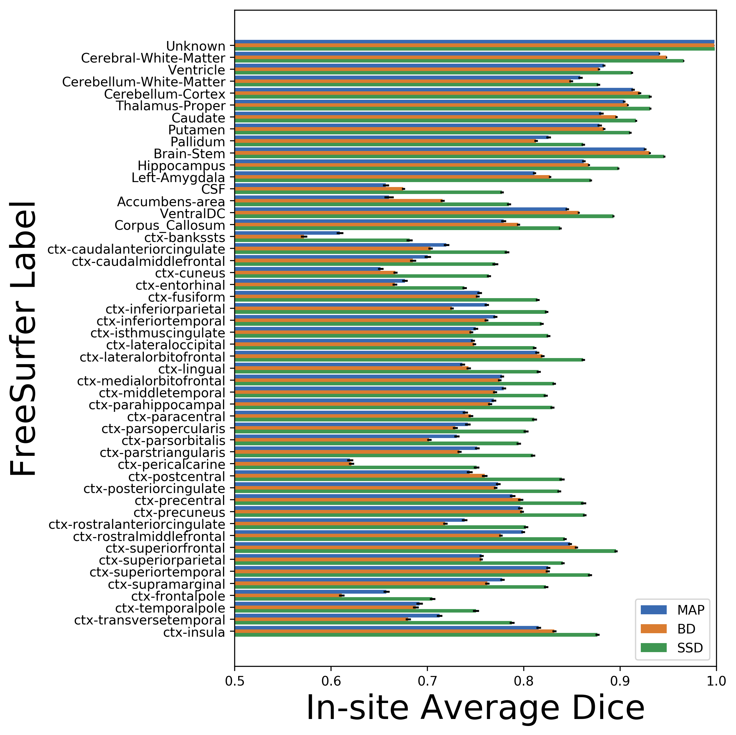 Figure 2
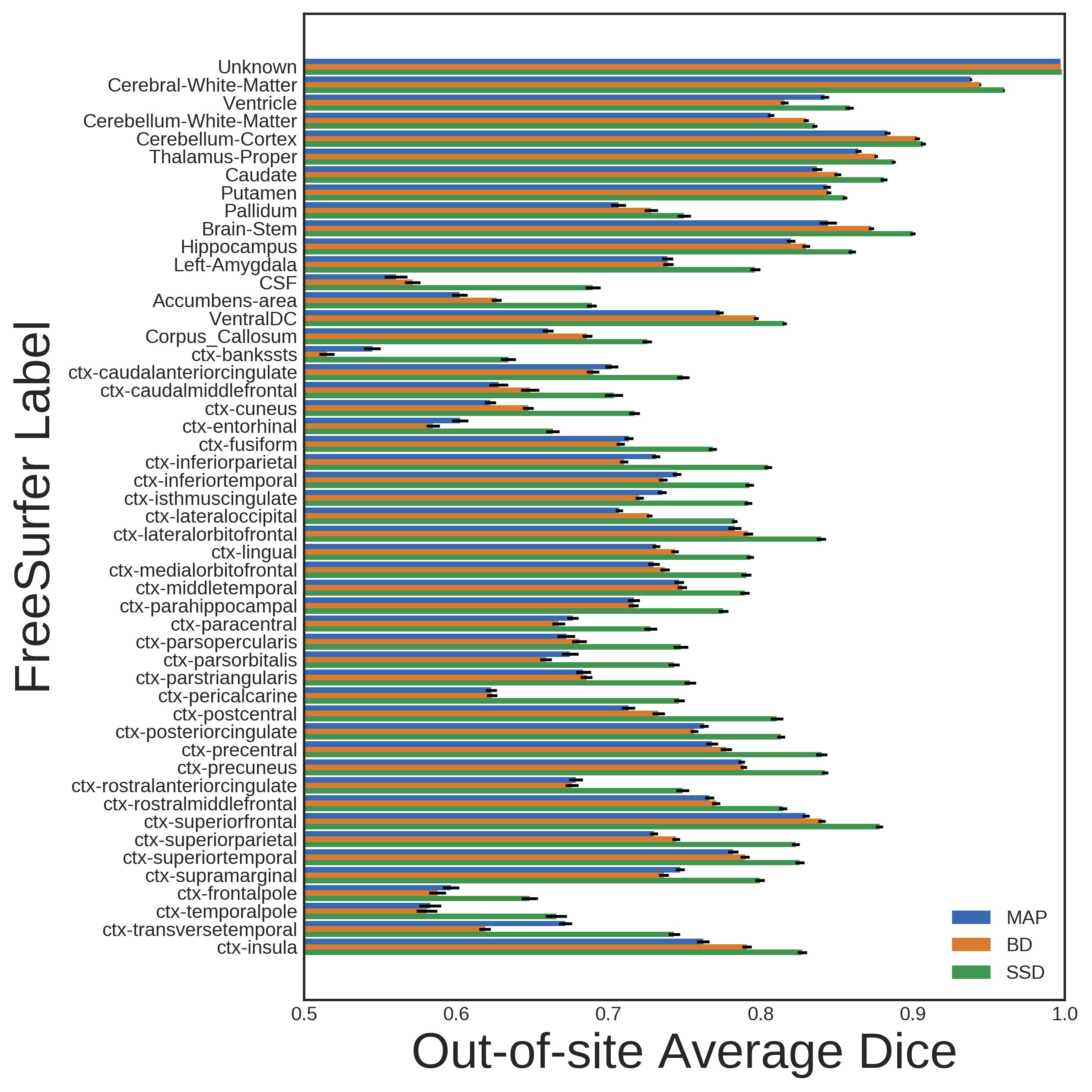 Figure 3
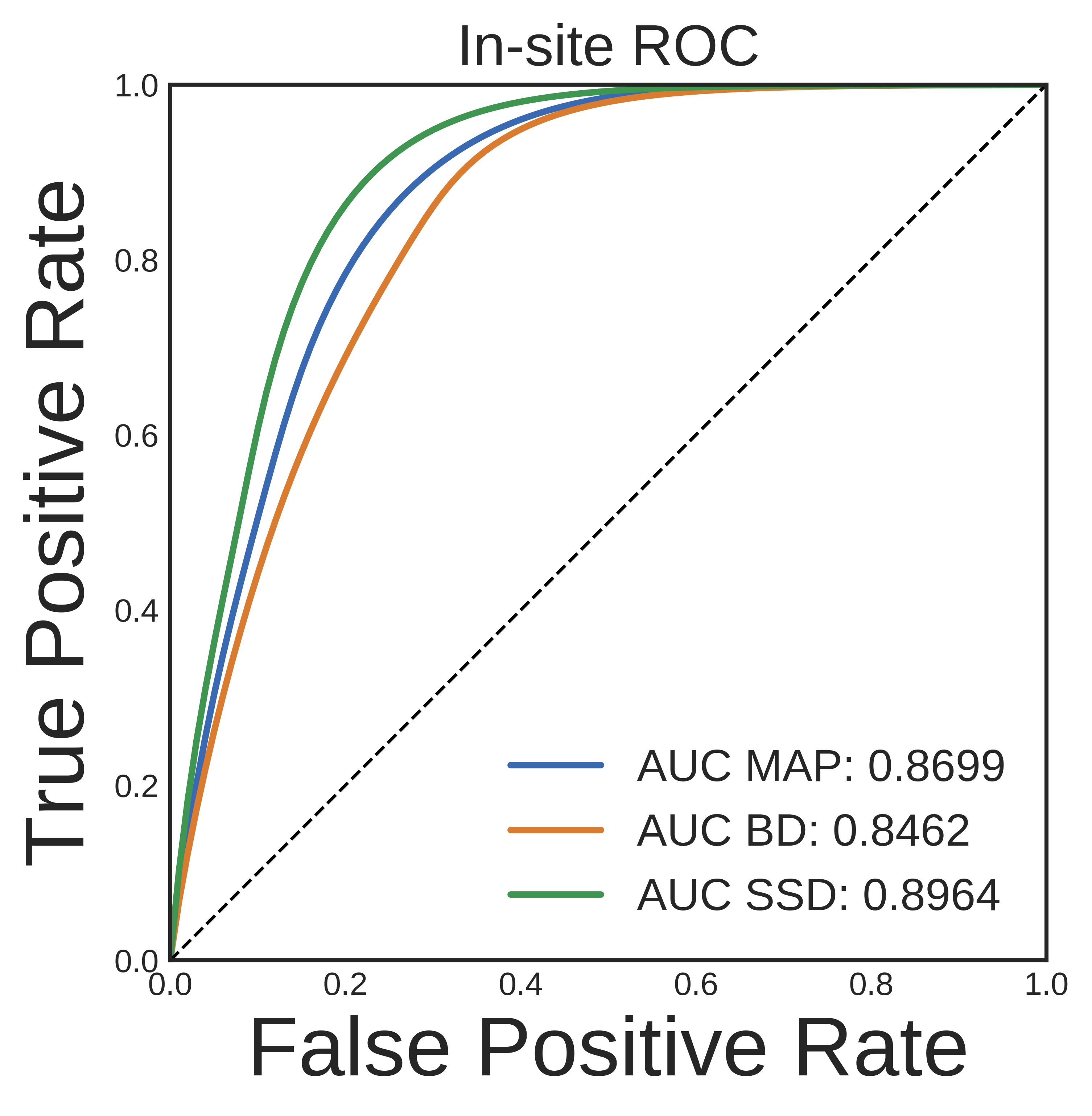 Figure 4
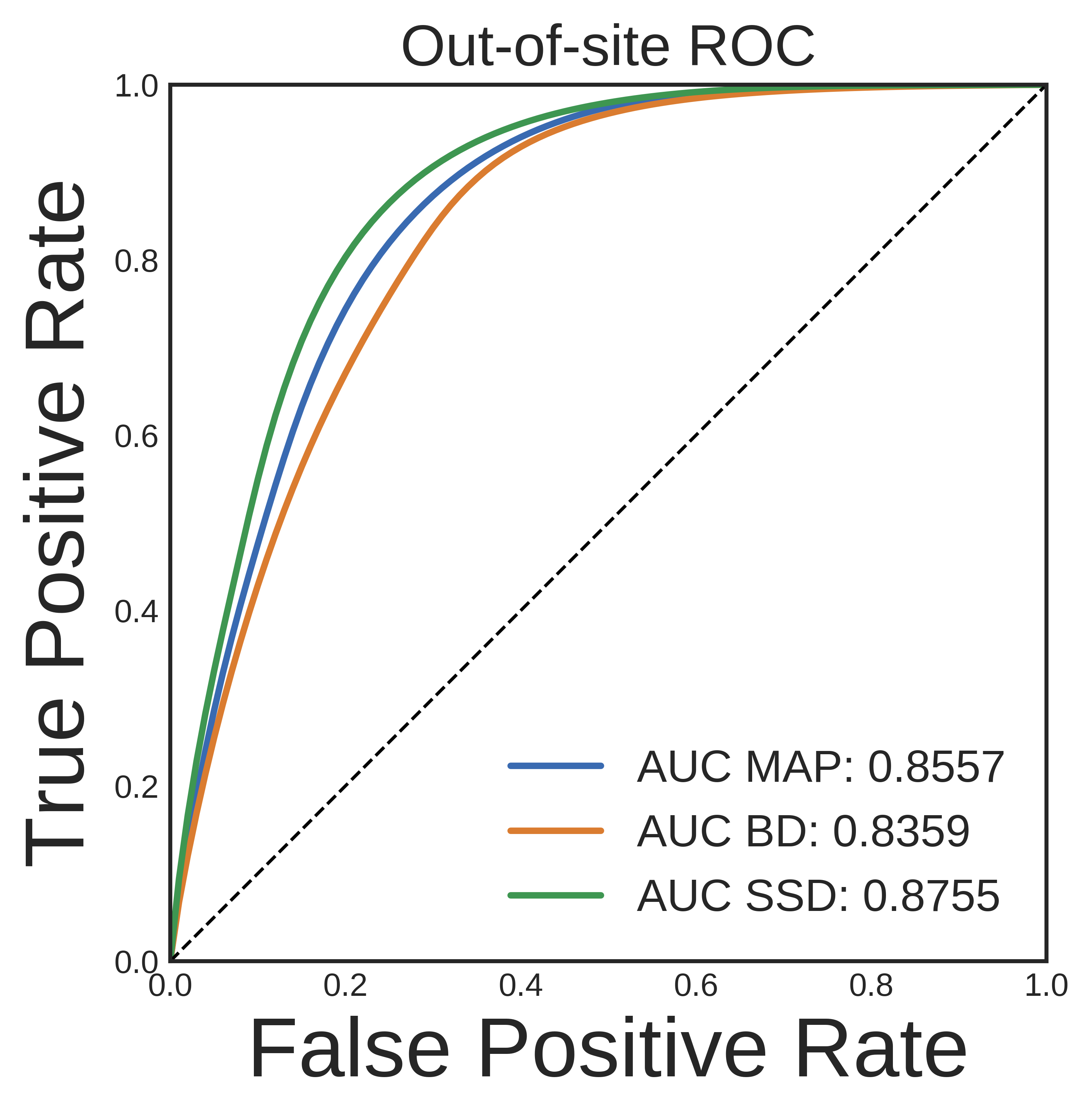 Figure 5
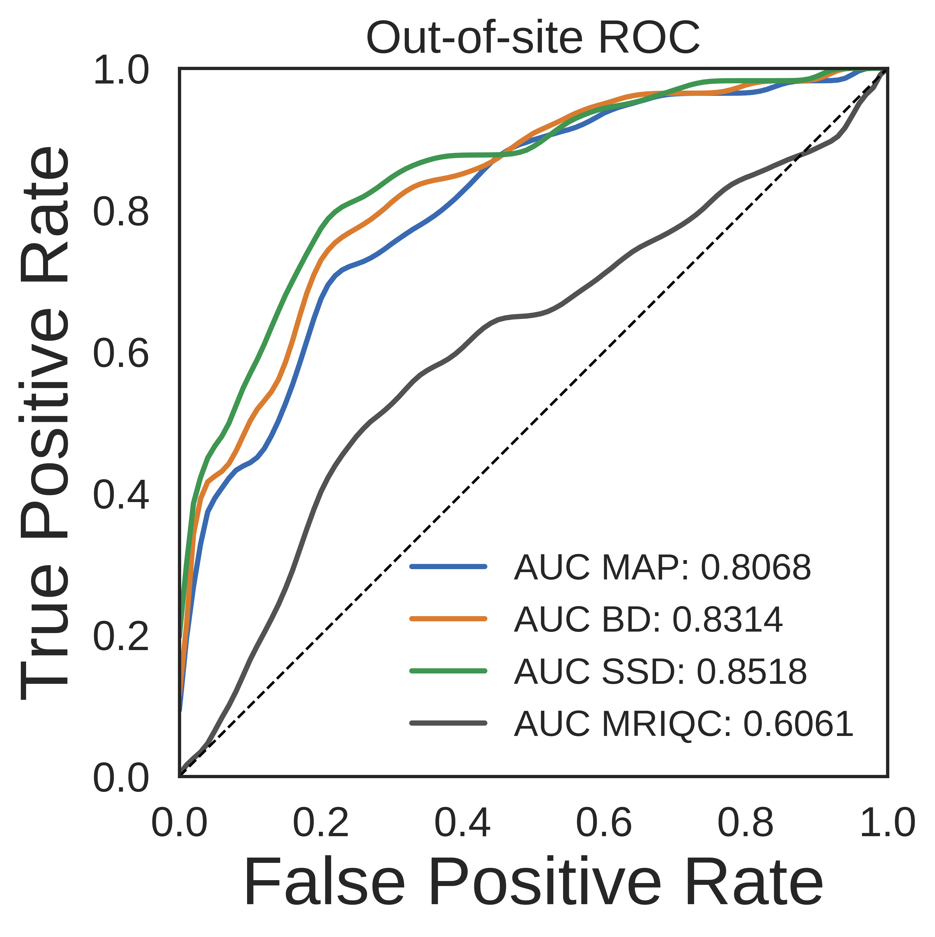 Figure 6
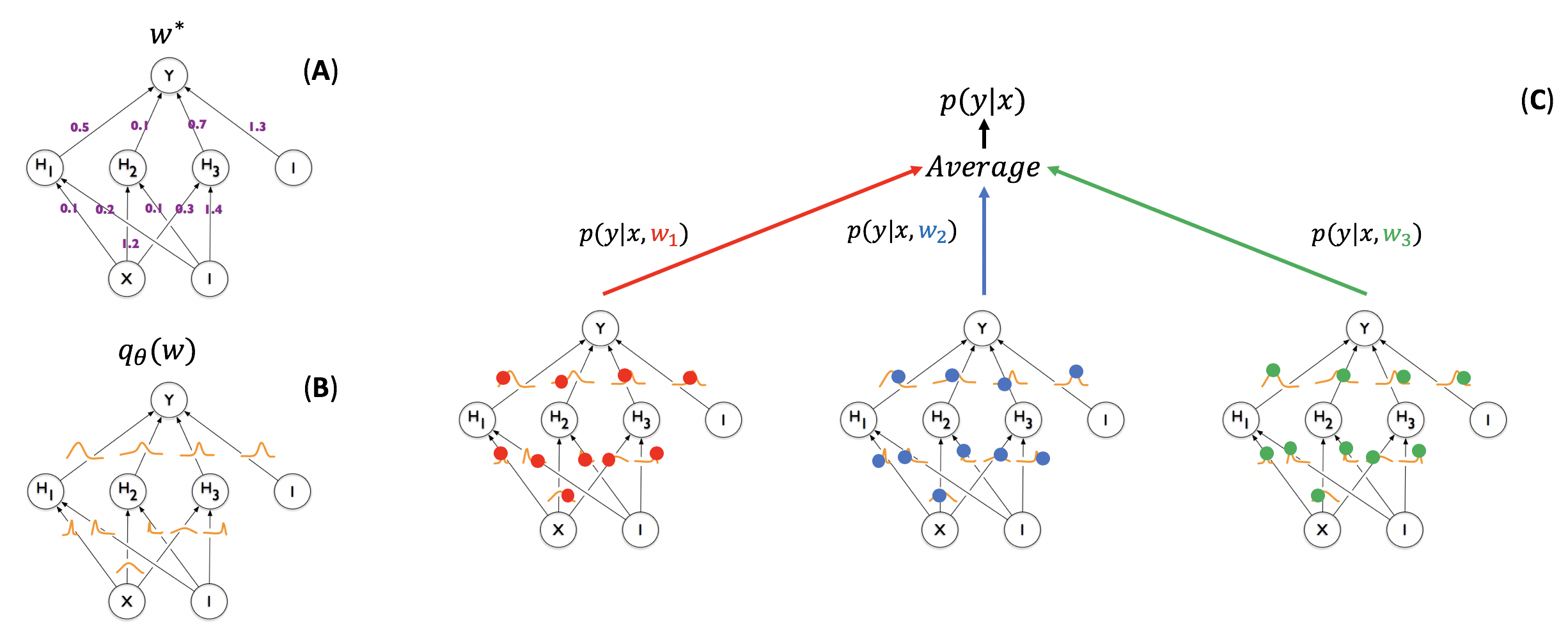 Figure 8
 Figure 9
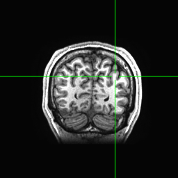 Figure 10
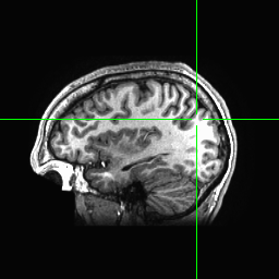 Figure 11
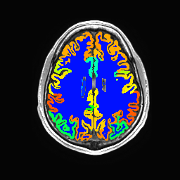 Figure 12
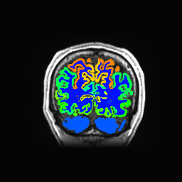 Figure 13
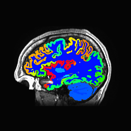 Figure 14
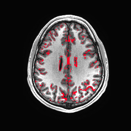 Figure 15
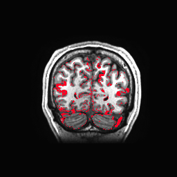 Figure 16
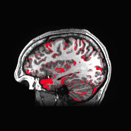 Figure 17
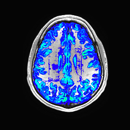 Figure 18
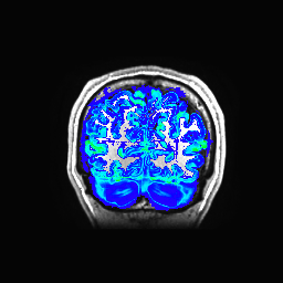 Figure 19
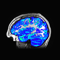 Figure 20
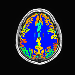 Figure 21
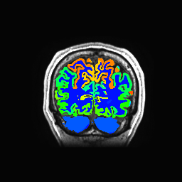 Figure 22
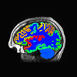 Figure 23
 Figure 24
 Figure 25
 Figure 26
 Figure 27
 Figure 28
 Figure 29
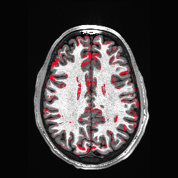 Figure 30
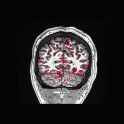 Figure 31
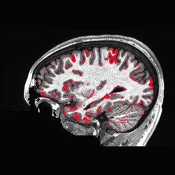 Figure 32
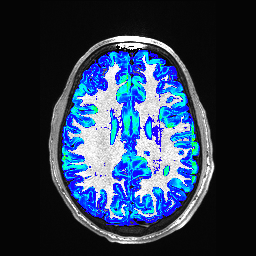 Figure 33
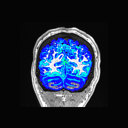 Figure 34
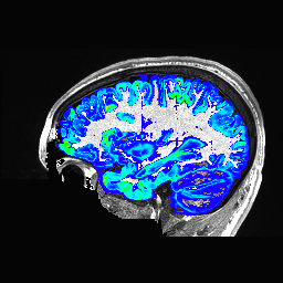 Figure 35
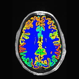 Figure 36
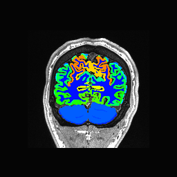 Figure 37
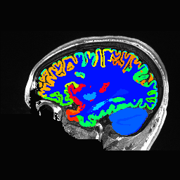 Figure 38
| Dataset | Number of Examples |
|---|---|
| CoRR (Zuo et al., 2014) | 3,039 |
| OpenfMRI (Poldrack et al., 2013) | 1,873 |
| NKI (Nooner et al., 2012) | 1,136 |
| SLIM (Liu et al., 2017) | 1,003 |
| ABIDE (Di Martino et al., 2014) | 992 |
| HCP (Van Essen et al., 2013) | 956 |
| ADHD200 (Bellec et al., 2017) | 719 |
| CMI (Alexander et al., 2017) | 611 |
| SALD (Wei et al., 2018) | 477 |
| Buckner (Biswal et al., 2010) | 183 |
| HBNSSI (O’Connor et al., 2017) | 178 |
| GSP (Holmes et al., 2015) | 152 |
| Haxby (Haxby et al., 2011; Nastase et al., 2017) | 55 |
| Gobbini (di Oleggio Castello et al., 2017) | 51 |
| ICBM (Mazziotta et al., 2001) | 45 |
| Barrios (Vázquez et al., 2016) | 10 |
| Layer | Filter | Padding | Dilation () | Non-linearity |
|---|---|---|---|---|
| 1 | 1 | 1 | ReLU | |
| 2 | 1 | 1 | ReLU | |
| 3 | 1 | 1 | ReLU | |
| 4 | 2 | 2 | ReLU | |
| 5 | 4 | 4 | ReLU | |
| 6 | 8 | 8 | ReLU | |
| 7 | 1 | 1 | ReLU | |
| 8 | 0 | 1 | Softmax |
| Method | In-site | Out-of-site |
|---|---|---|
| MAP | 0.7790 0.0576 | 0.7333 0.0498 |
| BD | 0.7764 0.0506 | 0.7369 0.0474 |
| SSD | 0.8373 0.0471 | 0.7921 0.0444 |
Peer Reviews
No public reviews on file for this paper yet. If you reviewed it on a platform where reviews are public (OpenReview, ICLR, NeurIPS, ICML), you can paste yours below so the community can read it here.
Code & Models
Videos
No videos yet. Explain this paper in a talk, walkthrough, or lecture? Add one.
\correspondance
\extraAuth
Knowing what you know in brain segmentation using Bayesian deep neural networks
Patrick McClure1,2, Nao Rho1,2, John A. Lee2,3, Jakub R. Kaczmarzyk4, Charles Zheng1,2, Satrajit S. Ghosh4, Dylan M. Nielson2,3, Adam G. Thomas3, Peter Bandettini2, Francisco Pereira1,2
Abstract
1
In this paper, we describe a Bayesian deep neural network (DNN) for predicting FreeSurfer segmentations of structural MRI volumes, in minutes rather than hours. The network was trained and evaluated on a large dataset (n = 11,480), obtained by combining data from more than a hundred different sites, and also evaluated on another completely held-out dataset (n = 418). The network was trained using a novel spike-and-slab dropout-based variational inference approach. We show that, on these datasets, the proposed Bayesian DNN outperforms previously proposed methods, in terms of the similarity between the segmentation predictions and the FreeSurfer labels, and the usefulness of the estimate uncertainty of these predictions. In particular, we demonstrated that the prediction uncertainty of this network at each voxel is a good indicator of whether the network has made an error and that the uncertainty across the whole brain can predict the manual quality control ratings of a scan. The proposed Bayesian DNN method should be applicable to any new network architecture for addressing the segmentation problem.
\helveticabold
2 Keywords:
brain segmentation, deep learning, magnetic resonance imaging, bayesian neural networks, variational inference, automated quality control
3 Introduction
Identifying which voxels in a structural magnetic resonance imaging (sMRI) volume correspond to different brain structures (i.e. segmentation) is an essential processing step in neuroimaging analyses. These segmentations are often generated using the FreeSurfer package (Fischl, 2012), a process which can take a day or more for each subject (FreeSurfer, 2018). The computational resources for doing this at a scale of hundreds to thousands of subjects are beyond the capabilities of the computational resources available to most researchers. This has led to an interest in the use of deep neural networks as a general approach for learning to predict the outcome of a processing task, given the input data, in a much shorter time period than the processing would normally take. In particular, several deep neural networks have been trained to perform segmentation of brain sMRI volumes (Ronneberger et al., 2015; Roy et al., 2018b; Fedorov et al., 2017b, a; Li et al., 2017; Dolz et al., 2018), taking between a few seconds and a few minutes per volume. These networks predict a manual or an automated segmentation from the structural volumes (Roy et al. (2018b), Fedorov et al. (2017b), Fedorov et al. (2017a), and Dolz et al. (2018) used FreeSurfer, and Petersen et al. (2010) used GIF (Cardoso et al., 2015)). These networks, however, have been trained on a limited number (on the order of hundreds) of examples from a limited number of sites (i.e. locations and/or scanners), which can lead to poor cross-site generalization for complex segmentation tasks with a large number of classes (McClure et al., 2018). This includes several of the recent DNNs proposed for fine-grain sMRI segmentation. (Note: We focus on DNNs which predict 30 classes.)
Roy et al. (2018b) performed 33 class segmentation using 581 sMRI volumes from the IXI dataset to train an initial model and then fine-tuned on 28 volumes from the MALC dataset (Marcus et al., 2007). They showed an approximately 9.4% average Dice loss on out-of-site data from the ADNI-29 (Mueller et al., 2005), CANDI (Kennedy et al., 2012), and IBSR (Rohlfing, 2012) datasets. Fedorov et al. (2017a) used 770 sMRI volumes from HCP (Van Essen et al., 2013) to train an initial model and then fine-tuned on 7 volumes from the FBIRN dataset (Keator et al., 2016). Li et al. (2017) performed a 160 class segmentation using 443 sMRI volumes from the ADNI dataset (Petersen et al., 2010) for training. Fedorov et al. (2017a) and Li et al. (2017) did not report test results for sites that where not used during training.
These results show that it is possible to train a neural network to carry out segmentation of a sMRI volume. However, they provide a limited indication of whether such a network would work on data from any new site not encountered in training. While fine-tuning on labelled data from new sites can improve performance, even while using small amounts of data (Fedorov et al., 2017a; Roy et al., 2018b; McClure et al., 2018), a robust neural network segmentation tool should generalize to new sites without any further effort. As part of the process of adding segmentation capabilities to the “Nobrainer” tool 111https://github.com/neuronets/nobrainer, we trained a network to predict FreeSurfer segmentations given a training set of 10,000 sMRI volumes. This paper describes this process, as well as a quantitative and qualitative evaluation of the performance of the resulting model.
Beyond the segmentation performance of the network, a second aspect of interest to us is to understand whether it is feasible for a network to indicate how confident it is about its prediction at each location in the brain. We expect the network to make errors, be it because of noise, unusual positioning of the brain, very different contrast than what it was trained on, etc. Because our model is probabilistic and seeks to learn uncertainties, we expect it to be less confident in its predictions in such cases. It is also possible that, for certain locations, there are very similar brain structures labelled as different regions in different people. In such locations, there would be a limit to how well the network could perform, the Bayes error rate (Hastie et al., 2005). Additionally, the network should be less confident for examples that are very different from those seen in the training set (e.g., contain large artifacts). While prediction uncertainty can be computed for standard neural networks, as done by Dolz et al. (2018), these uncertainty estimates are often overconfident (Guo et al., 2017; McClure and Kriegeskorte, 2017). Bayesian neural networks (BNNs) have been proposed as a solution to this issue. One popular BNN approach is Monte-Carlo (MC) Bernoulli Dropout (Srivastava et al., 2014; Gal and Ghahramani, 2016). Using this method, Li et al. (2017); Roy et al. (2018a) showed that the segmentation performance of the BNN predictions was better for voxels with low dropout sampling-based uncertainties and that injected input noise can lead to increased uncertainty. Roy et al. (2018a) also found that using MC Bernoulli dropout decreased the drop in segmentation performance from 9.4% to 7.8% on average when testing on data from new sites compared to Roy et al. (2018b). However, MC Bernoulli dropout does not learn dropout probabilities from data, which can lead to not properly modeling the uncertainty of the predicted segmentation. Recent works has shown that these dropout probabilities can be learned using a concrete relaxation (Gal et al., 2017). Additionally, learning individual uncertainties for each weight has been shown to be beneficial for many purposes (e.g. pruning and continual learning) (Blundell et al., 2015; Nguyen et al., 2018; McClure et al., 2018). In this paper, we propose using both learned dropout uncertainties and individual weight uncertainties.
Finally, we test the hypothesis that overall prediction uncertainty across an entire image reflects its “quality”, as measured by human quality control (QC) scores. Given the effort required to produce such scores, there have been multiple attempts to either crowdsource the process (Keshavan et al., 2018) or automate it (Esteban et al., 2017). The latter, in particular, does not rely on segmentation information, so we believe it is worthwhile to test whether uncertainty derived from segmentation is more effective.
4 Methods
4.1 Data
4.1.1 Imaging Datasets
We combined several datasets (Table 1), many of which themselves contain data from multiple sites, into a single dataset with 11,480 T1 sMRI volumes. In-site validation and test sets were created from the combined dataset using a 80-10-10 training-validation-test split. This resulted in a training set of 9,184 volumes, a validation set of 1,148 volumes, and a test set of 1,148 volumes. The training set was used for training the networks, the validation set for setting DNN hyperparameters (e.g, Bernoulli dropout probabilities), and the test set was used for evaluating the performance of the DNNs on new data from the same sites that were used for training.
We additionally used 418 sMRI volumes from the NNDSP dataset (Lee et al., 2018) as a held-out dataset to test generalization of the network to an unseen site. In addition to sMRI volumes, each NNDSP sMRI volume was given a QC score from 1 to 4, higher scores corresponding to worse scan quality, by two raters (3 if values differed by more than 1), as described in Blumenthal et al. (2002). If a volume had a QC score greater than 2, it was labeled as a bad quality scan; otherwise, the scan was labeled as a good quality scan.
4.1.2 Segmentation Target
We computed 50-class FreeSurfer (Fischl, 2012) segmentations, as in Fedorov et al. (2017a), for all subjects in each of the datasets described earlier. These were used as the labels for prediction. Although, FreeSurfer segmentations may not be perfectly correct, as compared to manual, expert segmentations, using them allowed us to create a large training dataset, as one could not feasibly label it by hand. FreeSurfer trained networks can also outperform FreeSurfer segmentations when compared to expert segmentations (Roy et al., 2018b). The trained network could be fine-tuned with expert small amounts of labeled data, which would likely improve the results (Roy et al., 2018b; McClure et al., 2018).
4.1.3 Data Pre-processing
The sMRI volumes were resampled to 1mm isotropic cubic volumes of 256 voxels per side and the voxel intensities were normalized according to Freesurfer’s mri_convert with the conform flag. After resampling, input volumes were individually z-scored across voxels. We then split each sMRI volume into 512 non-overlapping sub-volumes, similarly to (Fedorov et al., 2017b, a), to be used as inputs for the neural network. The prediction target is the corresponding segmentation sub-volume. This resulted in 512 pairs, , of sMRI and label sub-volumes, respectively, for each sMRI volume.
4.2 Convolutional Neural Network
4.2.1 Architecture
Several deep neural network architectures have been proposed for brain segmentation, such as U-net (Ronneberger et al., 2015), QuickNAT (Roy et al., 2018b), HighResNet (Li et al., 2017) and MeshNet (Fedorov et al., 2017b, a). We chose MeshNet because of its relatively simple structure, its lower number of learned parameters, and its competitive performance, since the computational cost of Bayesian neural networks scales based on structural complexity and number of parameters.
MeshNet uses dilated convolutional layers (Yu and Koltun, 2015) due to the 3D structural nature of sMRI data. Applying a discrete volumetric dilated convolutional layer to one input channel for one weight filter can be expressed as:
[TABLE]
where is the input to the layer, , , and are the bounds for the , , and axes of the filter with weights , is the voxel, , where the convolution is computed. The set of indices for the elements of can be defined as . The dilation factor, number of filters, and other details of the MeshNet-like architecture that we used for all experiments is shown in Table 2. Note that we increased the number of filters per layer from 72 to 96, compared to Fedorov et al. (2017a) and McClure et al. (2018), since we greatly increased the number of training volumes.
4.2.2 Maximum a Posteriori Estimation
When training a neural network, the weights of the network, , are often learned using maximum likelihood estimation (MLE). For MLE, is maximized where is the training dataset and is the th input-output example. This often overfits, however, so we used a prior on the network weights, , to obtain a maximum a posteriori (MAP) estimate, by optimizing :
[TABLE]
We used a fully factorized Gaussian prior (i.e. . This results in the MAP weights being learned by minimizing the softmax cross-entropy with L2 regularization. At test time, this point estimate approximation, , is used to make a prediction for new examples:
[TABLE]
4.2.3 Approximate Bayesian Inference
In Bayesian inference for neural networks, a distribution of possible weights is learned instead of just a MAP point estimate. Using Bayes’ rule, , where is the prior over weights. However, directly computing the posterior, , is often intractable, particularly for DNNs. As a result, an approximate inference method must be used.
One of the most popular approximate inference methods for neural networks is variational inference, since it scales well to large DNNs. In variational inference, the posterior distribution is approximated by a learned variational distribution of weights , with learnable parameters . This approximation is enforced by minimizing the Kullback-Leibler divergence (KL) between , and the true posterior, , , which measures how differs from using relative entropy. This is equivalent to maximizing the variational lower bound (Hinton and Van Camp, 1993; Graves, 2011; Blundell et al., 2015; Kingma et al., 2015; Gal and Ghahramani, 2016; Molchanov et al., 2017; Louizos and Welling, 2017), also known as the evidence lower bound (ELBO),
[TABLE]
where is
[TABLE]
and is the KL divergence between the variational distribution of weights and the prior,
[TABLE]
,
, which measures how differs from using relative entropy.
Maximizing seeks to learn a that explains the training data, while minimizing (i.e. keeping close to ) prevents learning a that overfits to the training data.
The objective function in Eq. 4 is usually impractical to compute for deep neural networks, due to both: (1) being a full-batch approach and (2) integrating over . (1) is often dealt with by using stochastic mini-batch optimization (Robbins and Monro, 1951) and (2) is often approximated using Monte Carlo sampling. As discussed in Graves (2011); Kingma et al. (2015), these methods can be used to perform stochastic gradient variational Bayes (SGVB) in deep neural networks. For each parameter update, an unbiased estimate of for a mini-batch, , is calculated using one weight sample, , from for each mini-batch example. This results in the following approximation to Eq. 4:
[TABLE]
where
[TABLE]
At test time, the weights, would ideally be marginalized out, , when making a prediction for a new example. However, this is often impractical to compute for DNNs, so a Monte-Carlo approximation is often used. This results in the prediction of a new example being made by averaging the predictions of multiple weight samples from (Figure 1):
[TABLE]
where .
MC Bernoulli Dropout
For MC Bernoulli dropout (BD) (Gal and Ghahramani, 2016), we drew weights from by drawing a Bernoulli random variable (), where are the indices of the volume axes, for every element of the layer, , input, , and then elementwise multiplying and before applying the next dilated convolutional layer. This effectively sets the filter weights to zero when applied to a dropped element. Gal and Ghahramani (2016) approximated the KLD between this Bernoulli variational distribution and a zero-mean Gaussian by replacing the variational distribution with a mixture of Gaussians, resulting in an L2-like penalty. However, this can lead to pathological behaviour due to Bernoulli distributions not having support over all real numbers (Hron et al., 2018). In Bernoulli dropout, codes for the uncertainty of the weights and is often set layerwise via hyperparameter search. (For our experiments, we found the best value of to be 0.9 after searching over the values of 0.95, 0.9, 0.75, and 0.5 using the validation set.) However, Bayesian models would ideally learn how uncertain to be for each weight.
Spike-and-Slab Dropout with Learned Model Uncertainty
We propose a form of dropout that both learns the dropout probability for each filter using a concrete relaxation of dropout (Gal et al., 2017), and an individual uncertainty for each weight using fully factorized Gaussian (FFG) filters (Graves, 2011; Blundell et al., 2015; Molchanov et al., 2017; Nguyen et al., 2018; McClure et al., 2018). This is in contrast to previous spike-and-slab dropout methods, which did not learn the model (or epistemic) uncertainty (Der Kiureghian and Ditlevsen, 2009; Kendall and Gal, 2017) from data either by learning the dropout probabilities or by learning the variance parameter of the Gaussian components of the weights (McClure and Kriegeskorte, 2017). In our proposed method, we assume each of the filters are independent (i.e. ), as done in previous FFG methods (Graves, 2011; Blundell et al., 2015; Molchanov et al., 2017; Nguyen et al., 2018; McClure et al., 2018). We then decompose each filter into a dropout-based component, , and a Gaussian component, , such that . Per this decomposition, we perform variational inference on the joint distribution of , instead of on p() directly (Titsias and Lázaro-Gredilla, 2011; McClure and Kriegeskorte, 2017). We then assume each element of is independent (i.e. ), and that each weight is Gaussian (i.e. ) with learned parameters and . Instead of drawing each from , we draw them from a concrete distribution (Gal et al., 2017) with a learned dropout probability, , for each filter:
[TABLE]
where . This concrete distribution converges to the Bernoulli distribution as the sigmoid scaling parameter, , goes to zero. (In this paper, we used .) As discussed in Kingma et al. (2015) and Molchanov et al. (2017), randomly sampling each for each mini-batch example can be computationally expensive, so we used the fact that the sum of independent Gaussian variables is also Gaussian to move the noise from the weights to the convolution operation, as in McClure et al. (2018). For, dilated convolutions and the proposed spike-and-slab variational distribution, this is described by:
[TABLE]
where
[TABLE]
[TABLE]
and
[TABLE]
For this spike-and-slab dropout (SSD) implementation, we used a spike-and-slab prior, instead of the Gaussian prior used by Gal and Ghahramani (2016) and Gal et al. (2017). Using a spike-and-slab prior with MC Bernoulli dropout was discussed in Gal (2016), but not implemented. As in the variational distribution, each filter is independent in the prior. Per the spike-and-slab decomposition discussed above, the KL-divergence term of the ELBO can be written as
[TABLE]
where are the learned parameters and and are priors. Assuming that each weight in a filter is independent, as commonly done in the literature (Graves, 2011; Blundell et al., 2015; Nguyen et al., 2018), allows the term to be rewritten as
[TABLE]
For , we used the KL-divergence between two Bernoulli distributions,
[TABLE]
since we used a relatively small sigmoid scaling parameter. Using ,
[TABLE]
For this paper, the spike-and-slab prior parameters were set as , , and . corresponds to a maximum entropy prior (i.e. in the absence of new data be maximally uncertain). Alternatively, a close to [math] is a sparcity prior (i.e. in the absence of data do not use a filter).
4.3 Implementation Details
The DNNs were implemented using Tensorflow (Abadi et al., 2016). During training, the parameters of each DNN were updated using Adam (Kingma and Ba, 2015) with an initial learning rate of 1e-4. A mini-batch size of 32 subvolumes was used with data parallelization across 4 12GB NVIDIA Titan X Pascal GPUs was used for training and a mini-batch size of 8 subvolumes on 1 12GB NVIDIA Titan X Pascal GPU was used for validation and testing.
4.4 Quantifying performance
4.4.1 Segmentation performance measure
To measure the quality of the produced segmentations, we calculated the Dice coefficient, which is defined by
[TABLE]
where is the binary segmentation for class produced by a network, is the ground truth produced by FreeSurfer, is the true positive rate for class , is the false negative rate for class , and is the false positive rate for class . We calculate the Dice coefficient separately for each class , and average across classes to compute the overall performance of a network for one sMRI volume.
4.4.2 Uncertainty measure
We quantify the uncertainty of a prediction, , using the aleatoric uncertainty (Der Kiureghian and Ditlevsen, 2009; Kendall and Gal, 2017), which was measured by the entropy of the softmax across the 50 output classes,
[TABLE]
We calculate the uncertainty for each output voxel separately, and the uncertainty for one sMRI volume by averaging across all output voxels not classified as background (i.e. given the unknown label).
5 Results
5.1 Segmentation performance
We trained MAP, MC Bernoulli Dropout (BD), and Spike-and-Slab Dropout (SSD) Meshnet-like CNNs on the 9,298 sMRI volumes in the training set. We then applied our networks to produce segmentations for both the in-site test set and the out-of-site test data. For the BD and SSD networks, 10 MC samples were used for test predictions. The means and standard deviations across volumes for the average Dice across all 50 classes are shown in Table 3. Dice scores for each label for the in-site and out-of-site test sets are shown in Figure 2 and 3, respectively. We found that, compared to MAP and BD, SSD significantly increased the Dice for both the in-site () and out-of-site () test sets, per a paired t-test across test volumes. We found that SSD had a 5.7% drop in performance from the in-site test set to the out-of-site test set, where as the MAP has a drop of 6.2% and BD a drop of 5.4%. This is better than drops of 9.4% and 7.8% on average reported in the literature by Roy et al. (2018b) and Roy et al. (2018a), respectively. In Figures 4 and 5, we show selected example segmentations for the SSD network for volumes that have Dice scores similar to the average Dice score across the respective dataset.
5.2 Utilizing Uncertainty
5.2.1 Predicting segmentation errors from uncertainty
Ideally, an increase in DNN prediction uncertainty indicates an increase in the probability that that prediction is incorrect. To evaluate whether this is the case for the trained brain segmentation DNN, we performed a receiver operating characteristic (ROC) analysis. In this analysis, voxels are ranked from most uncertain to least uncertain and one considers, at each rank, what fraction of the voxels were also misclassified by the network. An ROC curve can then be generated by plotting the true positive rate vs the false negative rate for different uncertainty thresholds used to predict misclassification. The area under this curve (AUC) typically summarizes the results of the ROC analysis. The average ROC and AUCs across volumes for MAP, BD, and SSD for the in-site and out-of-site test sets are shown in 6. Compared to MAP and BD, SSD significantly improved the AUC for both the in-site () and out-of-site () test sets, per a paired t-test across test set volumes.
5.2.2 Predicting scan quality from uncertainty
Ideally, the output uncertainty for inputs not drawn from the training distribution should be relatively high. This could potentially be useful for a variety of applications. One particular application is detection of bad quality sMRI scans, since the segmentation DNN was trained using relatively good quality scans. To test the validity of predicting high vs low quality scans, we performed an ROC analysis on the held-out NNDSP dataset, where manual quality control ratings are available. We also did the same analysis using MRIQC (v0.10.5) Esteban et al. (2017), a recently published method that combines a wide range of automated QC algorithms. To statistically test whether any method significantly outperformed the other methods, we performed bootstrap sampling of the AUC for predicting scan quality from average uncertainty by sampling out-of-site test volumes. We performed 10,000 bootstrap samples, each with 418 volumes. The average ROC and AUC for the MAP, BD, SSD, and MRIQC methods are shown in Figure 7. The MAP, BD, and SSD networks all have significantly higher AUCs than MRIQC (,, and , respectively). Additionally, SSD had a significantly higher AUC than both MAP and BD ( and , respectively).
6 Discussion
Segmentation of structures in sMRI volumes is a critical pre-processing step in many neuroimaging analyses. However, these segmentations are currently generated using tools that can take a day or more for each subject (FreeSurfer, 2018), such as FreeSurfer. This computational cost can be prohibitive when scaling analyses up from hundreds to thousands of subjects. DNNs have recently been proposed to perform sMRI segmentation is seconds to minutes. In this paper, we developed a Bayesian DNN, using spike-and-slab dropout, with the goals of increasing the similarity of the DNN’s predictions to the FreeSurfer segmentations and generating useful uncertainty estimates for these predictions.
In order to evaluate the proposed Bayesian network, we trained a standard deep neural network (DNN), using MAP estimation, to predict FreeSurfer segmentations from structural MRI (sMRI) volumes. We trained on a little under 10,000 sMRIs, obtained by combining approximately 70 different datasets (many of which, in turn, contain images from several sites, e.g. NKI, ABIDE, ADHD200). We used a separate test set of more than 1,000 sMRIs, drawn from the same datasets. The resulting standard DNN performs at the same level of state-of-the-art networks (Fedorov et al., 2017a). This result, however, was obtained by testing over an order of magnitude more test data, and many more sites, than those papers. We also tested performance on a completely separate dataset (NNDSP) from a site not encountered in training, which contained 418 sMRI volumes. Whereas Dice performance dropped slightly, this was less than what was observed in other studies (Roy et al., 2018b, a); this suggests that we may be achieving better generalization by training on our larger and more diverse dataset, and we plan on testing this on more datasets from novel sites in the future. This is particularly important to us, as this network is meant to be used within an off-the-shelf tool222https://github.com/neuronets/nobrainer.
We demonstrated that the estimated uncertainty for the prediction at each voxel is a good indicator of whether the standard network makes an error in it, both in-site and out-of-site. The tool that produces the predicted segmentation volume for an input sMRI will also produce an uncertainty volume. We anticipate this being useful at various levels, e.g. to refine other tools that rely on segmentation images, or to to improve prediction models based on sMRI data (e.g. modification of calculation of cortical thickness, surface area, voxel selection or weighting in regression (Roy et al., 2018a) or classification models, etc).
We also demonstrated that the average prediction uncertainty across voxels in the brain is an excellent indicator of manual quality control ratings. Furthermore, it outperforms the best existing automated solution (Esteban et al., 2017). Since automation is already used in large repositories (e.g. OpenMRI), we plan on offering our tool as an additional quality control measure.
Finally, we showed that a new Bayesian DNN using spike-and-slab dropout with learned model uncertainty was significantly better than previous approaches. This spike-and-slab method increased segmentation performance and improved the usefulness of output uncertainties compared both to a MAP DNN method and an MC Bernoulli dropout method, which has previously been used in the brain segmentation literature (Li et al., 2017; Roy et al., 2018a). These results show that Bayesian DNNs are a promising method for building brain segmentation and automated sMRI quality control tools. We have also made a version of “Nobrainer”, that incorporates the networks trained and evaluated in this paper, available for download and use within a Singularity/Docker container 333https://github.com/neuronets/kwyk.
We believe it may be possible to improve this segmentation processing, in that we did not use registration. One option would be to use various techniques for data augmentation (e.g. variation of image contrast, since that is pretty heterogeneous, rotations/translations of existing examples, addition of realistic noise, etc). Another would be to eliminate the need to divide the brain into sub-volumes, which loses some global information; this will become more feasible in GPUs with more memory. Finally, we plan on using post-processing of results (e.g. ensure some coherence between predictions for adjacent voxels, leverage off-the-shelf brain and tissue masking code).
Acknowledgments
This research was supported (in part) by the Intramural Research Program of the NIMH (ZICMH002968). This work utilized the computational resources of the NIH HPC Biowulf cluster. (http://hpc.nih.gov). JK’s and SG’s contribution was supported by NIH R01 EB020740.
The reference list from the paper itself. Each links out to its DOI / PubMed record.
- 1Abadi et al. (2016) Abadi, M., Barham, P., Chen, J., Chen, Z., Davis, A., Dean, J., et al. (2016). Tensorflow: A system for large-scale machine learning. In 12th { { \{ USENIX } } \} Symposium on Operating Systems Design and Implementation ( { { \{ OSDI } } \} 16) . 265–283
- 2Alexander et al. (2017) Alexander, L. M., Escalera, J., Ai, L., Andreotti, C., Febre, K., Mangone, A., et al. (2017). An open resource for transdiagnostic research in pediatric mental health and learning disorders. Scientific data 4, 170181
- 3Bellec et al. (2017) Bellec, P., Chu, C., Chouinard-Decorte, F., Benhajali, Y., Margulies, D. S., and Craddock, R. C. (2017). The neuro bureau adhd-200 preprocessed repository. Neuroimage 144, 275–286
- 4Biswal et al. (2010) Biswal, B. B., Mennes, M., Zuo, X.-N., Gohel, S., Kelly, C., Smith, S. M., et al. (2010). Toward discovery science of human brain function. Proceedings of the National Academy of Sciences 107, 4734–4739
- 5Blumenthal et al. (2002) Blumenthal, J. D., Zijdenbos, A., Molloy, E., and Giedd, J. N. (2002). Motion artifact in magnetic resonance imaging: implications for automated analysis. Neuroimage 16, 89–92
- 6Blundell et al. (2015) Blundell, C., Cornebise, J., Kavukcuoglu, K., and Wierstra, D. (2015). Weight uncertainty in neural networks. In International Conference on Machine Learning . 1613–1622
- 7Cardoso et al. (2015) Cardoso, M. J., Modat, M., Wolz, R., Melbourne, A., Cash, D., Rueckert, D., et al. (2015). Geodesic information flows: spatially-variant graphs and their application to segmentation and fusion. IEEE transactions on medical imaging 34, 1976–1988
- 8Der Kiureghian and Ditlevsen (2009) Der Kiureghian, A. and Ditlevsen, O. (2009). Aleatory or epistemic? does it matter? Structural Safety 31, 105–112
