Critical behavior of the quasi-periodic quantum Ising chain
P. J. D. Crowley, C. R. Laumann, A. Chandran

TL;DR
This paper investigates the critical phenomena of the quasi-periodic quantum Ising chain, revealing how spatial modulation influences universality classes, critical exponents, and excitation localization, with special cases showing unique behaviors.
Contribution
It provides a detailed analytic and numerical analysis confirming the QP-Ising universality class and explores special phase difference cases with distinct critical properties.
Findings
Logarithmic wandering coefficient governs critical exponents and localization length.
Special phase differences lead to unique localization and critical behaviors.
Generalized Aubry-André duality prevents localization at certain parameters.
Abstract
The interplay of correlated spatial modulation and symmetry breaking leads to quantum critical phenomena intermediate between those of the clean and randomly disordered cases. By performing a detailed analytic and numerical case study of the quasi-periodically (QP) modulated transverse field Ising chain, we provide evidence for the conjectures of Ref. [Crowley et. al. 2018] regarding the QP-Ising universality class. In the generic case, we confirm that the logarithmic wandering coefficient governs both the macroscopic critical exponents and the energy-dependent localisation length of the critical excitations. However, for special values of the phase difference between the exchange and transverse field couplings, the QP-Ising transition has different properties. For , a generalised Aubry-Andr\'e duality prevents the finite energy excitations from localising despite…
Click any figure to enlarge with its caption.
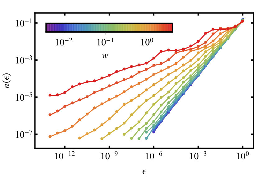 Figure 1
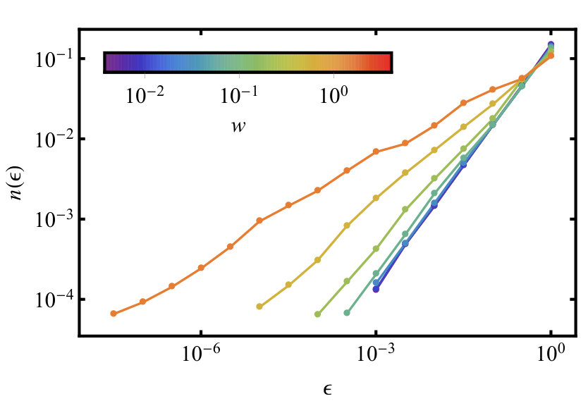 Figure 2
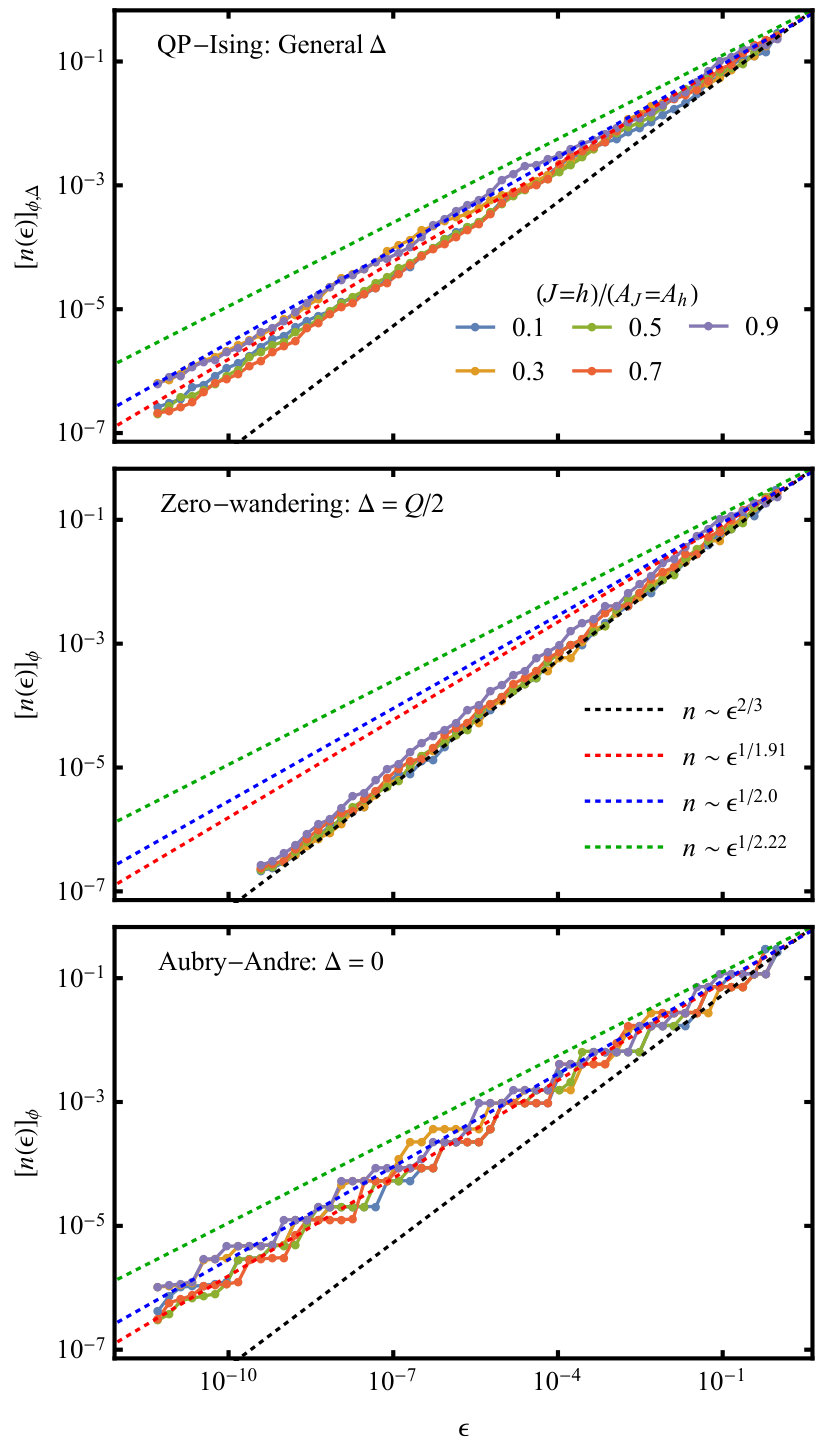 Figure 3
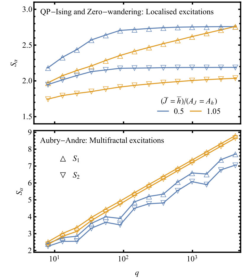 Figure 4
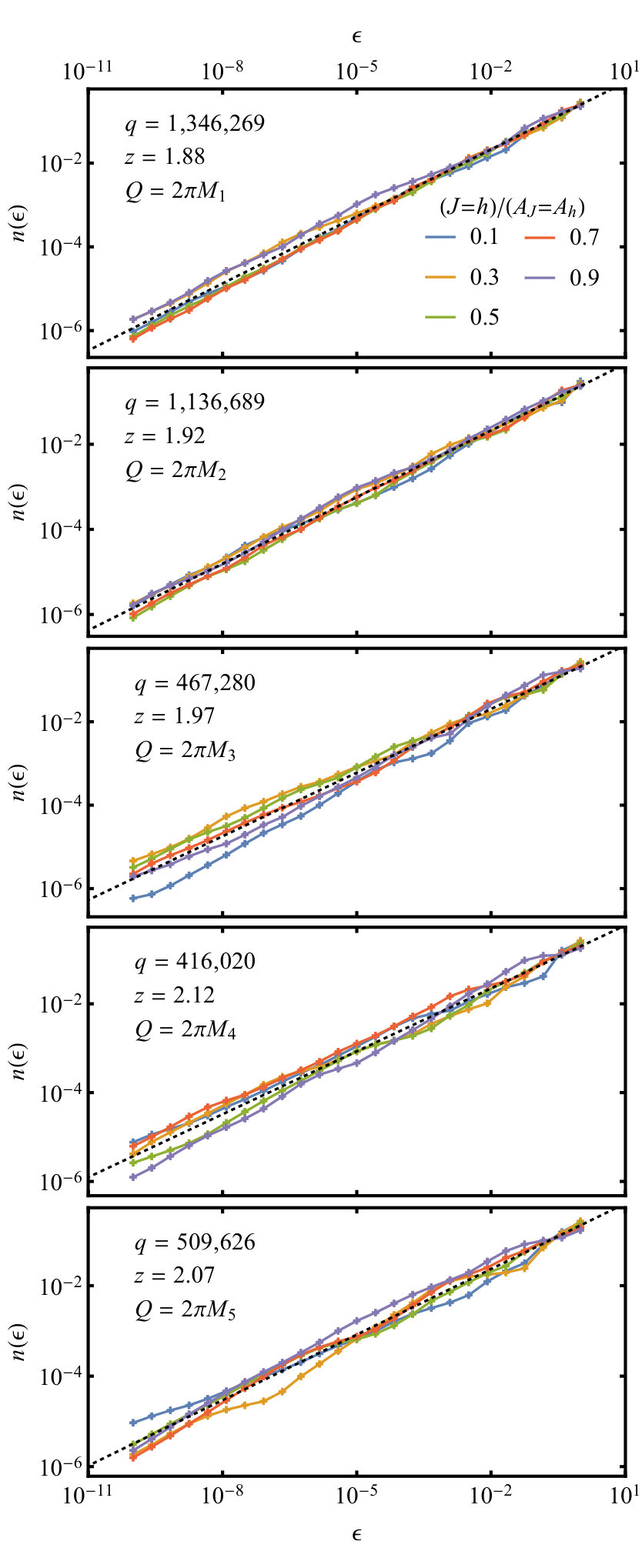 Figure 5
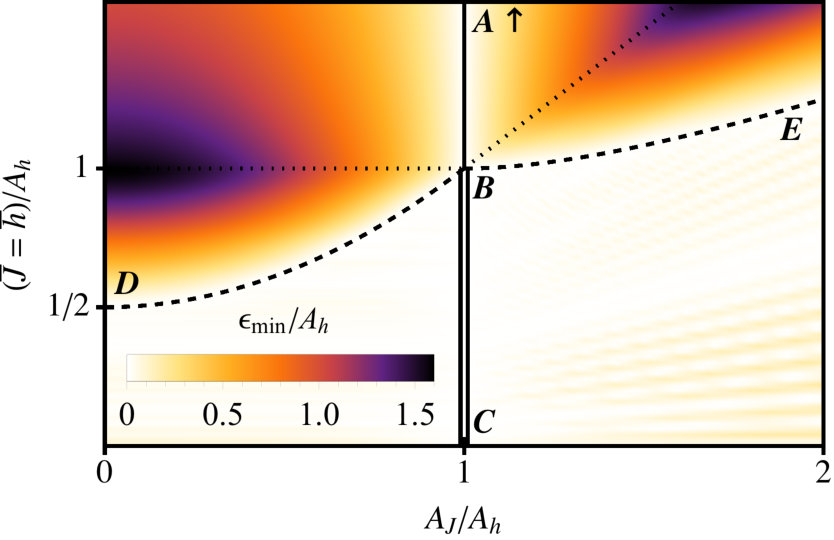 Figure 6
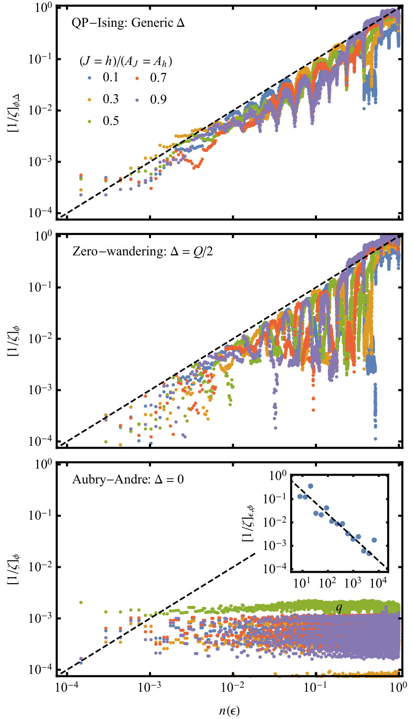 Figure 7
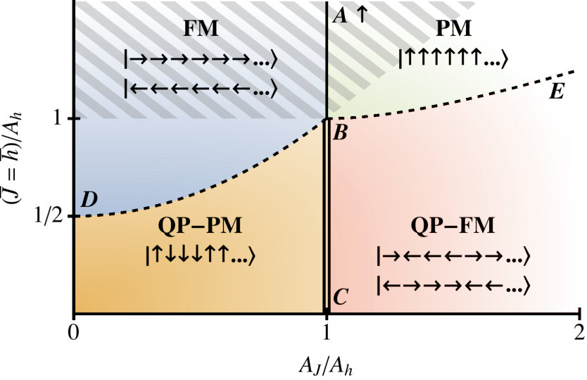 Figure 8
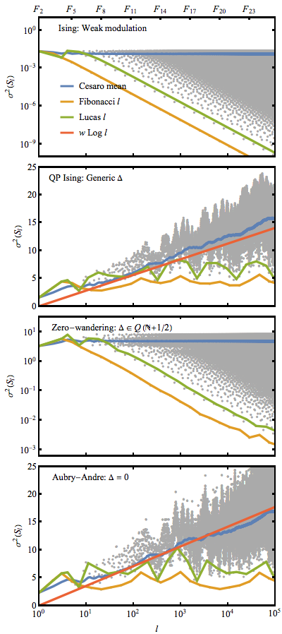 Figure 9
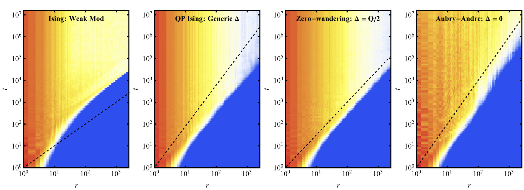 Figure 10
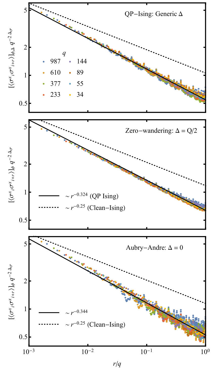 Figure 11
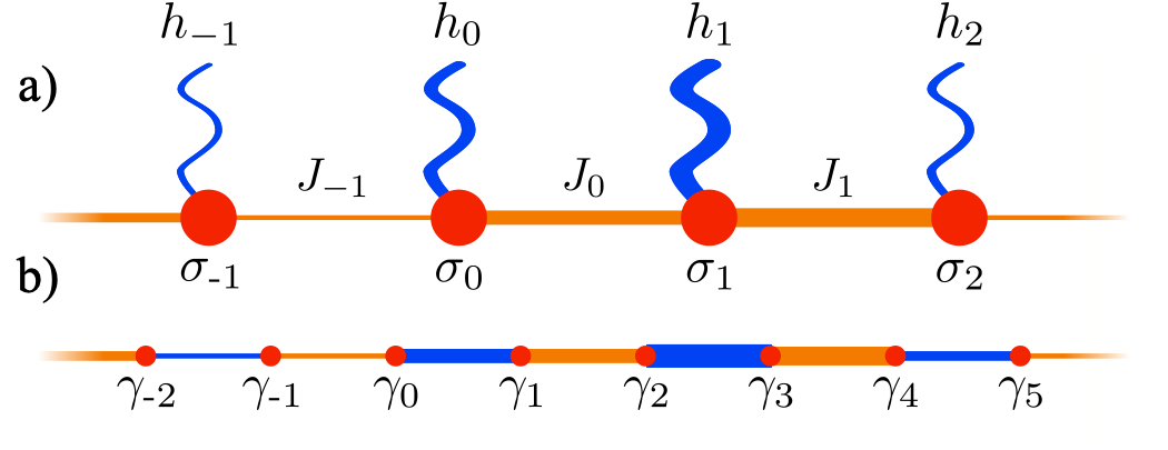 Figure 12
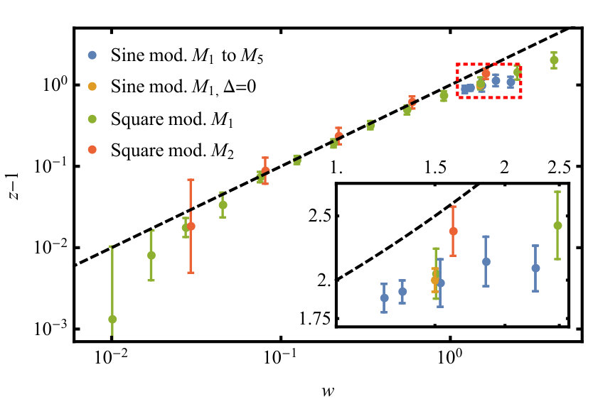 Figure 13
| Case | ||||||
|---|---|---|---|---|---|---|
| 0. | Ising (Weak modulation) | 0 | – | |||
| 1. | QP-Ising (Generic ) | |||||
| 2. | Zero-wandering () | 0 | ||||
| 3. | Aubry-André () | – |
| Spatial structure of low energy excitations | ||
| Delocalised | Localised | |
| Ising | Clean or periodic modulation Lieb et al. (1961); Onsager (1944) | |
| Weak-continuous-QP modulation Luck (1993a) | ||
| Fine-tuned discontinuous-QP Doria and Satija (1988); Iglói (1988); Ceccatto (1989); Kolář et al. (1989); Benza (1989); Benza et al. (1990); Luck (1993a); Grimm and Baake (1996); Hermisson et al. (1997); Iglói et al. (1997, 1998); Hermisson and Grimm (1998) | Strongly hyper-uniform random disorder Crowley et al. (2018b) | |
| QP-Ising | Aubry-André strong-continuous-QP modulation () | |
| Generic-discontinuous-QP modulation | Generic strong-continuous-QP modulation (), (See also Chandran and Laumann (2017); Crowley et al. (2018a)) | |
| Infinite | ||
| randomness | — | Independent random disorder Fisher (1992, 1995, 1999) |
| Weakly hyper-uniform random disorder Crowley et al. (2018b) | ||
Peer Reviews
No public reviews on file for this paper yet. If you reviewed it on a platform where reviews are public (OpenReview, ICLR, NeurIPS, ICML), you can paste yours below so the community can read it here.
Videos
No videos yet. Explain this paper in a talk, walkthrough, or lecture? Add one.
Critical behavior of the quasi-periodic quantum Ising chain
P. J. D. Crowley
Department of Physics, Boston University, Boston, MA 02215, USA
C. R. Laumann
Department of Physics, Boston University, Boston, MA 02215, USA
A. Chandran
Department of Physics, Boston University, Boston, MA 02215, USA
Abstract
The interplay of correlated spatial modulation and symmetry breaking leads to quantum critical phenomena intermediate between those of the clean and randomly disordered cases. By performing a detailed analytic and numerical case study of the quasi-periodically (QP) modulated transverse field Ising chain, we provide evidence for the conjectures of Ref. Crowley et al. (2018a) regarding the QP-Ising universality class. In the generic case, we confirm that the logarithmic wandering coefficient governs both the macroscopic critical exponents and the energy-dependent localisation length of the critical excitations. However, for special values of the phase difference between the exchange and transverse field couplings, the QP-Ising transition has different properties. For , a generalised Aubry-André duality prevents the finite energy excitations from localising despite the presence of logarithmic wandering. For such that the fields and couplings are related by a lattice shift, the wandering coefficient vanishes. Nonetheless, the presence of small couplings leads to non-trivial exponents and localised excitations. Our results add to the rich menagerie of quantum Ising transitions in the presence of spatial modulation.
I Introduction
In the vicinity of a quantum Ising phase transition in a spatially homogeneous (clean) system, the magnetisation (the order parameter) fluctuates on the respective macroscopic length and time scales,
[TABLE]
where and are the correlation length and dynamic exponent respectively, and is the control parameter which measures the deviation from the transition Goldenfeld (1992). These fluctuations of the order parameter are mediated by long wavelength, low energy excitation modes. In the clean transverse field Ising model (TFIM) the transition is in the celebrated Onsager universality class with Onsager (1944); Suzuki et al. (2012).
Spatial modulation of the couplings can change the universality class of a quantum phase transition. One feature of this is that locally different regions of the system may be closer to, further from, or even on different sides of, the critical point . This is quantified by , the local deviation from the transition point at the spatial position . If the fluctuations of the spatially averaged in a region of size grow sufficiently quickly with , then the clean transition is perturbatively unstable by the Harris-Luck criterion Harris (1974); Luck (1993a, b). Accordingly, random modulation destabilises the clean Ising transition and ultimately the system flows to an infinite-randomness critical point McCoy and Wu (1968, 1969); Shankar and Murthy (1987); Fisher (1992, 1995, 1999); Motrunich et al. (2000). Both quasi-periodic and hyper-uniform modulation allow the fluctuations of to be tuned, and can send the system to new fixed points Tracy (1988); Kolář et al. (1989); Benza et al. (1990); Lin and Tao (1992); Luck (1993a); Turban et al. (1994); Grimm and Baake (1996); Hermisson et al. (1997); Iglói et al. (1997, 1998); Hermisson and Grimm (1998); Crowley et al. (2018a, b).
For sufficiently strong smooth quasi-periodic (QP) modulation of the couplings in the TFIM, Ref. Crowley et al. (2018a) showed that the fluctuations of , the wandering, grow logarithmically with region size :
[TABLE]
The logarithmic growth violates the Harris-Luck criterion but not strongly enough to drive the system to infinite randomness. Ref. Crowley et al. (2018a) argued that the resulting QP-Ising transitions belonged to a new line of intermediate fixed points parameterised by . At the QP-Ising transitions, macroscopic observables obey power-law scaling (as in the clean Ising transition but with distinct scaling data), while the finite energy excitations are localised (as in the disordered Ising transition). Table 2 summarises the critical behaviours of the clean, QP modulated and disordered Ising transitions which have been studied in the literature. Case 1 in Table 1 provides representative values of the critical exponents for the QP-Ising transition with a specific .
In this article, we extend the study of Ref. Crowley et al. (2018a) and provide evidence in support of two conjectures:
- (A)
The logarithmic wandering coefficient captures the microscopic detail necessary to determine the macroscopic critical exponents of the QP-Ising transition. That is, parameterises a line of critical fixed points. 2. (B)
The finite energy excitations are localised with a localisation length which diverges as with the same dynamical exponent as that governing the equilibrium correlations. Thus, up to logarithmic corrections.
While the two conjectures are generically true at the QP-Ising transition, fine tuning can violate either of them. The Zero-Wandering case and Aubry-André case (Cases 2 and 3 in Table 1) provide examples of finely tuned models that violate the first and second conjecture respectively.
A challenge in the study of QP models is to separate physically robust observables from the mathematically intriguing tower of multi-fractal turtles on which they ride. Our approach is to focus on the macroscopic exponents which govern spatially averaged response and neglect the highly structured scale-dependent fluctuations about the mean trends in any given correlator. Thus, we supplement a calculation of with measurements of the dynamical exponent and susceptibility exponent . sets the low temperature behaviour of the specific heat and is extracted from the global density of states , while controls the divergence of the susceptibility to a longitudinal field , and is extracted from spatially averaged two-point correlation functions using scaling relations.
The paper is structured as follows. We first review the QP-TFIM (Sec. II) and its equilibrium properties (Sec. III). We then calculate the logarithmic wandering for different values of and show that strong-smooth modulation violates the Harris-Luck criterion (Sec. IV). In Sec. V, we compute and for the QP-Ising transition and provide evidence in support of conjecture A in smooth and square-wave modulated TFIMs. We also compute the critical exponents for the Zero-wandering and Aubry-André transitions, and show that conjecture A is violated for the zero-wandering transition. In Sec. VI, we turn to the localisation properties of the Fermionic excitations. We show that the excitations are localised with at the zero-wandering and the QP-Ising transitions, but are critically delocalised at the Aubry-André transition. The Aubry-André transition therefore violates conjecture B. We end in Sec. VI.5 with striking dynamical consequences of the localisation for wave-packet spreading.
II Preliminaries
II.1 Model
The Hamiltonian of the one-dimensional QP-TFIM Chandran and Laumann (2017); Crowley et al. (2018a) is
[TABLE]
Here are the usual Pauli matrices, represents a longitudinal field which we henceforth set , and the couplings and are obtained from sampling -periodic functions and with wave-number . Quasi-periodicity requires that the ratio of the wavelength to the lattice length is irrational:
[TABLE]
Our analysis focuses on pure tone sinusoidal modulation:
[TABLE]
where without loss of generality. This model is depicted in Fig. 1a. The results for the single tone case easily generalise to generic continuous , . In Tab. 2 and generally, if either of , has zeroes, the modulation is termed strong-QP; whereas if either has discontinuities it is termed discontinuous-QP.
The QP-TFIM (with ) is Ising-symmetric. That is, for . The ground state phases are classified according to this symmetry: the paramagnetic (PM) phase is Ising symmetric, while in the ferromagnetic (FM) phase the symmetry is spontaneously broken.
The QP-TFIM satisfies Ising duality. Under the transformation:
[TABLE]
the QP-TFIM with couplings , maps to another QP-TFIM with couplings , . Thus any self dual points coincide with phase transitions.
II.2 Commensurate approximation
We may approach the limit of QP (i.e. incommensurate) modulation through a series of commensurate approximations , where the co-prime integers constitute the th best rational approximation to the irrational . The best rational approximations to an irrational are those which minimise over all rationals with a denominator no larger than . The incommensurate limit is obtained on taking .
As per the elementary results of Diophantine approximation Cassels (1957), the best approximations are given by truncating the continued fraction expansion,
[TABLE]
at the th level. For specificity, we focus on the Golden Ratio , for which the best rational approximations are where are the Fibonacci numbers. However, our results are readily generalisable to equal to any badly approximable number. Badly approximable numbers are defined by the property that is finite.
In the commensurate approximation, the QP-TFIM (3) is invariant under translations by lattice sites. The modes of the system are Bloch waves which can be calculated exactly in the infinite system limit . On length scales , the scaling properties of correlation functions is controlled by the critical properties of QP-Ising universality class, whereas on scales the periodicity is apparent, and the scaling of correlations is correspondingly dictated by the Onsager universality class. Thus plays the role of a finite size cut-off to the QP-Ising transition.
II.3 Jordan-Wigner transformation to Majorana fermions
Using the Jordan-Wigner transformation
[TABLE]
the QP-TFIM (3) maps to a quadratic Hamiltonian (see Fig 1b):
[TABLE]
where are Majorana fermions satisfying . The antisymmetric-Hermitian matrix has non-zero elements only for . The eigenvalues of come in pairs , whose corresponding eigenvectors are related by complex conjugation . Let label the positive eigenvalues. Define the Majorana fermions:
[TABLE]
where . Re-writing in terms of these Majorana fermions
[TABLE]
Above, the complex fermions encode the excitations of the TFIM.
II.4 Spatial structure of excitation modes
Transport properties, such as the thermal conductivity, are dictated by the spatial structure of excitations above the ground state.
In the clean TFIM, is translationally invariant, and the are delocalised Bloch waves. This give rise to ballistic spreading of energy which is locally injected into the system. In non-interacting one-dimensional models, random modulation leads to exponentially localised excitations each with some localisation centre and localisation length Anderson (1958).
Similar localisation of all excitations is seen in the equilibrium phases of randomly modulated Pfeuty (1979), or strongly QP modulated Ising chains Chandran and Laumann (2017); Crowley et al. (2018a). At the transition, the modulation-induced localisation competes with the development of long-range order, which necessitates an extended soft mode at zero energy. This forces to diverge as a function of energy
[TABLE]
In mesoscopic systems, this produces a vanishing fraction of delocalised low energy states with . Certain QP-modulation leads to excitations with fractal structure Kohmoto and Banavar (1986); Kohmoto et al. (1987); Hiramoto and Abe (1988); Fujiwara et al. (1989); Hiramoto and Kohmoto (1992); Han et al. (1994); Piéchon (1996). Wavepackets formed from fractal modes spread sub-ballistically but without bound Ketzmerick et al. (1997), so they are delocalised.
II.5 Scaling limit and scaling content
At a phase transition, correlation functions become scale free Goldenfeld (1992). In the vicinity of the transition, single parameter scaling posits that correlation functions are controlled by a single length scale and time scale which both diverge at the transition:
[TABLE]
Above, is the average deviation from the transition, and and are respectively the correlation length and dynamic critical exponents. Here, and throughout the manuscript, denotes spatial averaging (averaging over the site index). The dynamic critical exponent also controls the long-wavelength features of the dispersion and the low energy features of the density of states .
In a homogeneous system (), the scales determine the correlations in the vicinity of the transition
[TABLE]
where is the spin scaling dimension and denotes the connected part of the ground state correlator. In a spatially inhomogeneous systems, varies with the position . One can define mean and typical correlators by taking either the spatial arithmetic-mean or the spatial geometric-mean respectively, and these may display different scaling behaviour Fisher (1992, 1995, 1999); Motrunich et al. (2000); Crowley et al. (2018b).
In this manuscript, we focus on the mean correlators, as these determine macroscopic physical quantities via linear response. These mean correlators similarly define scaling functions
[TABLE]
where we have included the dependence on the period of commensurate modulation (see Sec. II.2), which functions much like a finite size cut-off. The critical data of the inhomogeneous case may be altered from the homogeneous case.
The susceptibility to a longitudinal field is an example of a physical quantity controlled by a mean correlator. This diverges at the critical point . Differentiating the free energy density we find
[TABLE]
The dependence on can be scaled out of the above integral, yielding the relation
[TABLE]
This provides a means to access susceptibility exponent from the scaling of spatially averaged correlation functions. The clean TFIM is a well-known example of the Onsager universality class Onsager (1944) with exponents , , and .
III Phase diagram of the QP-TFIM
III.1 Magnetic ordering of the phases
We highlight an interesting slice, , of the ground state phase diagram of the QP-TFIM Eq. (3) in Fig. 2. There are four phases. When typical exchange coupling is larger than the typical field the system magnetically orders Pfeuty (1979). In the magnetically ordered phases if the couplings are weakly modulated, , the phase is the usual gapped FM phase of the clean TFIM, and neighbouring spins align. However, if the couplings are strongly modulated, , the system is in the gapless QP-FM phase in which spins either align or anti-align with their neighbours depending on the sign of the . By duality the analogous statements hold for the PM and QP-PM phases which occur when the fields are weakly () or strongly () modulated respectively.
In the FM and PM phases, the local magnetizations (eg. and ) vary smoothly as the global couplings are tuned. In contrast in the QP-PM and QP-FM phases, these observables are sensitive to small changes to the global couplings (i.e. ) as these lead to sign reversals in the local couplings. Nonetheless, suitably spatially averaged observables vary smoothly within these phases and can satisfy scaling near the critical boundaries.
Figure 4 shows a density plot of the excitation gap across the same phase diagram as Fig. 2. As usual, the FM and PM phases are gapped. The QP-FM phase is gapless because of the density of arbitrarily weak bonds across which the Ising ordering direction can locally flip at low energy and similarly for the QP-PM phase. We note that the QP-Ising transition can take place between gapped QP-modulated phases when the coupling function has jump discontinuities.
III.2 QP-FM Order parameter and experimental signatures
It is well known that the FM phase spontaneously spontaneously breaks the symmetry and selects one of the two degenerate ground states in which the spins are either aligned or anti-aligned to the -axis. This long-range magnetic order is manifest in the non-zero value of the symmetry broken order parameter where is the normalised magnetisation.
As in the FM, in the QP-FM, the system spontaneously selects one of the two degenerate ground states related by the global spin flip. In these ground states neighbouring spins are aligned or anti-aligned according to the sign of the couplings . The order parameter
The effect of sign structure is easily removed by considering the absolute value of spin-spin correlations, yielding the corresponding order parameter for the QP-FM phase .
Formally is
For condensed matter realisations of the QP-Ising model, as with the anti-ferromagnet, experimental signatures of the order are evident in neutron scattering experiments which probe the structure factor
[TABLE]
In the QP-FM limit, , the ground state correlations are given by and where there are an even (odd) number of negative spin couplings in region . Thus as is varied the value of flips sign on average every sites, where is the fraction of negative couplings. This order persists over long distances and leads to a peak in at , where
[TABLE]
This peak is visible in Fig. 3, upper panel. This peak in at non-trivial is a clear signature of the quasi-periodic order and is not seen in the random Ising model which exhibits a single peak at when the are predominantly positive, and when they are predominantly negative.
For non-zero , the ground state correlations are accessible only numerically, we see the peak in the structure factor persists throughout the QP-FM phases, before decreasing and disappearing at the transition (Fig.3, lower panel).
III.3 Majorana [math]-modes and phase boundaries
The precise phase boundaries can be identified most easily by analysing the Majorana edge modes. In the thermodynamic limit of the FM and QP-FM phases, two of the Majorana eigen-modes and have zero energy,
[TABLE]
In the fermionic language, and are the unpaired topological edge modes of the Kitaev chain Kitaev (2001), whereas in the TFIM, they encode the two symmetry breaking ground states.
Expanding Eq. (20) in the basis of local fermions , the coefficients satisfy the two recursion relations
[TABLE]
Any linear combination of , yields a valid zero mode. Choosing and to be localised at opposite ends of the chain, one finds that has support only on odd sites, and has support only on even sites: , .
The localisation length controls the decay of the edge modes into the bulk of the chain . Solving for the localisation length of the left mode one finds
[TABLE]
Here the local reduced coupling is
[TABLE]
At the transition out of the symmetry breaking phase, the zero modes mix into bulk modes and cease to exist. For the edge modes to mix with bulk modes their localisation length must diverge. This gives the condition for criticality
[TABLE]
Eq. (24) corresponds to the familiar condition for the critical point of the random TFIM Pfeuty (1979).
As the sequence is equi-distributed on the interval , we may re-cast the sum in Eq. (24) into an integral:
[TABLE]
The zeros of this integral may be obtained analytically Chandran and Laumann (2017). In the plane, this yields the phase boundaries
[TABLE]
These lines are shown in Fig. 2. They meet at the bi-critical point . Under the action of the duality transformation (6) the line (26a) is self dual, whereas (26b) and (26c) are interchanged.
Note that the phase boundaries depend only on the energetic scales of the model, and are independent of the wave vector and the phases and .
IV Wandering of QP modulation
The primary effect of quasi-periodic modulation on the critical TFIM is captured by the its wandering. In this section, we define and analyse the wandering itself and in Sec. V we consider the implications for the critical data.
The wandering records the variation of the reduced coupling when summed over regions of finite length . The Onsager universality of the clean TFIM may persist in the presence of modulation only if a criterion due to Harris Harris (1974) and Luck Luck (1993a, b) is satisfied. We find generic strong continuous and discontinuous QP modulation violates this criterion, albeit much more weakly than random modulation, and thus leads to universality which is intermediate to the clean and random cases.
IV.1 Distinct cases analysed
Up to this point, our analysis has applied to the QP-TFIM irrespective of the value of the phase difference . However, on the self-dual critical boundary , when the value takes special rational values lead to fine tuned critical behaviour, distinct from the generic case. Thus, we separate our discussion into the following cases (cf. Table 1):
Ising: When , the modulation is weak and irrelevant to the clean Ising transition Luck (1993a, b), independent of . 2. 1.
QP Ising: For strong modulation ( or ) with generic on the critical lines , , , the universality class of the transition is QP-Ising, with universal content completely determined by the wandering coefficient Crowley et al. (2018a). 3. 2.
Zero-Wandering: For strong modulation on the self-dual boundary () with for , the wandering coefficient vanishes due to fine tuning and the Harris-Luck criterion is satisfied by the clean Ising transition. However, we find that the critical data are nonetheless modified and the system behaves as if in the QP-Ising class but with a broken relationship between wandering and critical exponents. 4. 3.
Aubry-André: Strong modulation with on the self-dual boundary , the wandering coefficient is again finite and we find the equilibrium scaling content is described by the generic QP-Ising transition (Case 1). However, the excitations are de-localised at all energies due to an Aubry-André type symmetry.
IV.2 Harris-Luck Criterion
The Harris-Luck criterion concerns the behaviour of the wandering, which is defined as the sum of reduced couplings over a region of length
[TABLE]
This quantity characterises the local deviation from criticality over the region, . has mean value and typical fluctuations of scale , with
[TABLE]
We decompose the local averaged reduced coupling into its mean value, and fluctuations about the mean
[TABLE]
where is some number dependent on microscopic details. It is clear that cannot converge to its mean value in the limit of large if the fluctuations are asymptotically larger than mean. This imposes the consistency condition
[TABLE]
To see how this condition bounds the critical exponents, set to , the length-scale up to which the critical point controls the ground state correlations. This recasts (30) as the Harris-Luck criterion for the stability of the transition to spatial modulation:
[TABLE]
Random modulation provides a useful example. In this case whilst in the clean TFIM . These quantities violate (31), indicating that in the vicinity of the transition, the fluctuations in on the length scale are too large to determine the phase of the system. Random modulation is therefore a relevant perturbation to the clean Ising transition. The random Ising chain flows to an infinite-randomness critical point with Fisher (1992, 1995, 1999), the minimal value which satisfies (31).
IV.3 Case 0: Ising
In the QP-TFIM, we use the equivalence of spatial averages , and phase averages to recast in a simple form:
[TABLE]
Above, the Fourier coefficient is defined as:
[TABLE]
The values of in the weakly modulated regime (, ) are depicted in Fig. 5 (upper panel, grey dots). We see that is a non monotonic function, bounded by its asymptotically separated infimum and supremum
[TABLE]
Here is equivalent to for some finite and all sufficiently large . Certain sub-series saturate the lower scaling bound, for example in Fig. 5 (upper panel) scales as its infimum when is a Fibonacci (gold line) or Lucas (green line) number.
As the infimum and supremum are asymptotically separated, we characterise the scaling behaviour by the Cesàro mean
[TABLE]
In the weakly modulated regime
[TABLE]
for some constant . At the clean Ising transition and the Harris-Luck criterion (31) is not violated either by the supremum or the Cesáro mean. The clean Ising transition is therefore stable to the introduction of weak QP modulation Luck (1993a, b).
IV.4 Case 1: QP-Ising
In the strongly modulated regime, is a non-monotonic function with an asymptotically separated infimum and supremum (Fig 5, second panel, grey)
[TABLE]
As in the weakly modulated case, the Fibonacci (gold line) and Lucas (green line) numbers follow the infimum. The Cesàro mean scales logarithmically
[TABLE]
where is the logarithmic wandering coefficient. The Harris-Luck criterion (31) is violated and the critical lines , and the parabolic phase boundaries and shown in Fig. 2 all have critical behaviour distinct from the clean model.
IV.4.1 Intuition for -wandering
The log-wandering originate from the logarithmic divergence in (33). In a region of size running over sites site , the values of the reduced coupling are set by evaluated at . These values are sufficiently uniformly distributed over the interval that we can gain intuition from considering as analogous to the Riemann sum
[TABLE]
Shifting the region of interest by varying moves this roughly uniformly lattice of values around, and induces fluctuations on this Riemann sum, these fluctuations are analogous to quantity . When is bounded and continuous, these fluctuations are , whereas when has a logarithmic divergence, the fluctuations are dominated by how close one samples to the divergence and one finds Crowley et al. (2018a).
IV.4.2 The logarithmic wandering coefficient
The logarithmic wandering coefficient controls the strength of the violation of the Harris-Luck criterion. As determines the universal content of the QP-Ising transition Crowley et al. (2018a), we derive its precise value below. From the definition of (38), the Cesàro mean (35) and (32)
[TABLE]
For strongly modulated smooth couplings, the zeros in , imply that
[TABLE]
The logarithmic growth of the sum (41) with is due to exponentially spaced terms, which appear when the denominator takes an small value.
Eq. (40) can be simplified. We note first that the series is a quasi-periodic in and has the following values on the different critical lines
[TABLE]
where is the th Chebyshev polynomial of the first kind. The properties of the line follow by duality from . In all cases of (42), if is rationally independent of , and , then the terms of the sum in (40) uniformly sample the values of and (40) factorises as
[TABLE]
The Cesàro mean of can be evaluated on the various critical lines,
[TABLE]
The second factor,
[TABLE]
Refs. Crowley et al. (2018a); Speyer showed that this limit converges to a finite value for equal to any badly approximable number. For example, in the case , may be exactly evaluated Crowley et al. (2018a); Speyer
[TABLE]
This calculation of is readily generalised to other quadratic numbers. Putting it all together for ,
[TABLE]
IV.5 Case 2: Zero wandering
For with the wandering coefficient is zero due to an exact cancellation. As the exchange and field couplings are related by a lattice shift , the sum separates into two boundary pieces for ,
[TABLE]
As a result, for all and the Harris-Luck bound (31) is not violated. Nevertheless, we will see later that this zero-wandering transition is not in the clean Ising universality class, due to the presence of small couplings.
IV.6 Case 3: Aubry-André
For on the line , the calculation proceeds similarly the QP-Ising case (Sec. IV.4), and the wandering grows logarithmically as in Eq. (38), with a slightly enhanced value of .
The calculation of is distinct only in technical details. Specifically,
[TABLE]
The factor is always for close to an odd integer, and always small for close to an even integer. The largest contribution to the sums in (40) comes from these terms.
As the factor is not self-averaging in the manner that allowed the factorisation (43) we must instead absorb this term into the sum .
This results in the factorisation (as before in (43)) for (for which ), and
[TABLE]
V Equilibrium Critical Exponents
We now discuss the consequences of the wandering analysis for the equilibrium critical exponents. The QP Ising and Aubry-André cases have logarithmic wandering and are in the QP Ising universality class of Ref. Crowley et al. (2018a). Remarkably, the zero-wandering transition also has modified critical data. We support the analysis in this section with numerical measurements.
V.1 Correlation length exponent
We saw in section IV.2 that the Harris-Luck criterion sets a condition which must be satisfied for the phase transition to be stable to additional spatial modulation. Consistent with the finding in the randomly modulated TFIM Fisher (1992, 1995, 1999); Crowley et al. (2018b), we conjecture that, as in the randomly disordered case, the correlation length exponent is altered so that the Harris-Luck criterion is saturated
[TABLE]
Applying (51) to the generic QP-Ising and Aubry-André transitions we find
[TABLE]
That is , when is defined as and + denotes a logarithmic correction. In contrast, for the zero-wandering transition, the correlation length of the clean Ising transition satisfies (51) and .
V.2 Specific heat and dynamical exponent
In the vicinity of the transition, the integrated density of states obeys the following scaling
[TABLE]
We use this relationship to estimate analytically by extracting the low energy integrated density of states from a leading order approximation of the secular equation.
A macroscopic way to measure the dynamical exponent is provided by the low-temperature heat capacity
[TABLE]
Here is the Fermi-Dirac distribution. For power law density of states ,
[TABLE]
V.2.1 QP-Ising (Generic ) and AA () transition
The following calculation proceeds identically for generic and because they both have logarithmic wandering .
Consider the excitation spectrum of the QP-TFIM. For finite period , this spectrum consists of states with band index , momentum and energy . Let be the highest energy of the th band, thus
[TABLE]
Thus the top of the lowest band lies at an energy . We note is the root of smallest magnitude of the characteristic polynomial , where
[TABLE]
This allows us to estimate by truncating to quadratic order
[TABLE]
From the form of the coefficients are found to be
[TABLE]
At the transition, . We therefore find
[TABLE]
where and is given by (27). As we are interested in the maximum energy of the [math]th band, we set . This yields
[TABLE]
To make progress it is necessary to approximate further. We: (i) neglect the correlations between the numerator and the denominator of the summand, (ii) replace the denominator with a single characteristic energy scale , and (iii) treat the as Gaussian independently distributed variables with mean and variance . This neglects correlations between for different , and non-Gaussianity of each . Making this approximation yields
[TABLE]
By (58) this estimate implies that and hence . Using the results of Sec. IV.4.2 for , we obtain
[TABLE]
for the QP-Ising transition on the critical line .
In Fig. 6 this prediction is compared with numerics. The data is compared with extracted values for indicated by the dashed lines. Specifically, in each case we extract values of by a least squares fit to the relationship
[TABLE]
The values of are computed exactly using the method of Refs. Schmidt (1957); Eggarter and Riedinger (1978), for . The numerics confirms the power law behaviour with an exponent , giving some discrepancy with the estimate (63). The power law behaviour of the integrated DOS is additionally confirmed numerically for other choices of in the supplementary material.
V.2.2 Zero-wandering transition ()
When , we have the relation . Equation (60) simplifies to
[TABLE]
Assuming that the sum is dominated by the minimal coupling , we obtain
[TABLE]
Thus, . In Fig. 6, we see that this agrees well with numerics.
The argument presented here is easily generalised to for generic and predicts provided . The estimate agrees well with numerics for general (data not shown).
V.2.3 Variation of the dynamical exponent with logarithmic wandering coefficient
The QP-Ising case describes the transition for generic . Ref. Crowley et al. (2018a) conjectured that the QP-Ising critical exponents are a function of the logarithmic wandering coefficient alone. This conjecture is confirmed by Fig. 7. Fig. 7 includes data for sine wave modulation (5) with , the th metallic mean (blue) for (data in Fig. 11 in Supp. Mat.) 111 The metallic number is the number whose continued fraction expansion coefficients are all the integer . ; sine wave modulation with , (gold) (data in Fig 6); and square wave modulation with (green) and (red), (data in Fig. 12 in Supp. Mat.).
The extracted values of support the conjecture that is a function of alone across a variety of QP-modulated models. Furthermore, the analytical estimate (black dotted line) is a good approximation to over intermediate values of . The deviation at low is a finite size effect, while at large , the crudeness of the approximation becomes apparent.
The square wave data in Fig. 7 is calculated from systems in which the couplings and fields take two values , according to a QP sequence. This sequence is constructed in exactly the same way as the sinusoidal case: but with chosen to be -periodic square waves. The square wave wandering analysis (see Supp. Mat.) is a simple extension of the sinusoidal case (Sec. IV), and similarly yields logarithmic wandering. The key difference from the sinusoidal case is that the square wave logarithmic wandering coefficient has continuous parametric dependence on the ratios (see Supp. Mat.). Thus for square waves may be continuously tuned to zero by taking without leaving the QP-Ising universality class. The ability to continuously tune allows a more extensive exploration of the relationship .
The square wave wandering analysis generalises mutatis mutandis to the case of any QP sequence in which the couplings take values drawn from a finite alphabet , . Thus generically such sequences have logarithmic wandering. However, we note that there are fine tuned sequences which also have no wandering (see Supp. Mat. App. D1b) Doria and Satija (1988); Iglói (1988); Ceccatto (1989); Kolář et al. (1989); Benza (1989); Benza et al. (1990); Luck (1993a); Grimm and Baake (1996); Hermisson et al. (1997); Iglói et al. (1997, 1998); Hermisson and Grimm (1998), analogous to the fine tuned Zero-wandering case. The methodology we present allows the study of TFIMs modulated by generic QP sequences whereas previous analyses have been restricted to special sequences which satisfy an inflation rule Doria and Satija (1988); Iglói (1988); Tracy (1988); Ceccatto (1989); Kolář et al. (1989); Benza (1989); Benza et al. (1990); Lin and Tao (1992); Luck (1993a); Turban et al. (1994); Grimm and Baake (1996); Hermisson et al. (1997); Iglói et al. (1997, 1998); Hermisson and Grimm (1998); Oliveira Filho et al. (2012); Yessen (2014).
V.3 Magnetic susceptibility and the scaling dimension
We turn to the value of the scaling dimension in the different cases. In terms of macroscopic properties of the system, controls the divergence with of the magnetic susceptibility to a longitudinal field . Near the critical point with an exponent
[TABLE]
The relationship (67) is Fishers scaling law in dimensions. The relation follows directly from the free energy in Eqs. (16) and (17).
We extract by minimising the mean deviation of over for to . We also verify data collapse for the extracted values of in Fig. 8. In the QP-Ising and Zero wandering cases we find , consistent with Ref. Crowley et al. (2018a) which studied only the QP-Ising case. The Aubry-André case has slightly enhanced wandering coefficient as compared to the QP-Ising value and consequently a slightly enhanced scaling dimension . The extracted values of and yield the values in the QP-Ising, Zero-wandering and Aubry-André cases respectively. These are are larger than the Onsager value of at the clean Ising transition (see Tab. 1).
VI Localisation of excitations
On the critical boundary, the TFIM possesses an extended zero energy mode. The zero mode is described by Eq. (21), which has infinite localisation length at the critical point (cf. Eq. (22))
[TABLE]
In the unmodulated TFIM, the zero mode is uniform; it arises as the zero energy and momentum limit of linearly dispersing fermionic low energy excitations. With QP modulation, the mode need not be spatially uniform. Nevertheless, it cannot be localised. There are accordingly several scenarios for the structure of the low energy excitations:
- •
The modes may remain ballistic, in which case the total bandwidth of the Bloch bands remains finite as the incommensurate limit is taken. The wavefunctions are uniformly extended with small spatial fluctuations.
- •
The modes may become multifractal; vanishes as a non-trivial power law in the incommensurate limit, but the finite energy inverse localisation length remains zero .
- •
The finite energy modes may localise, so long as the localisation length diverges as :
[TABLE]
In this case, the total bandwidth in any small energy window at finite energy decays exponentially with .
We find that all three of these scenarios are realised. When the QP modulation is irrelevant to the clean Ising transition (Ising case), the low energy excitations are ballistic. With strong modulation, the excitations generically localise with a localisation exponent which coincides with that extracted from the equilibrium density of states (QP-Ising and Zero-wandering cases). This agrees with the behaviour found in previous QP Crowley et al. (2018a); Chandran and Laumann (2017) and random Fisher (1992, 1995, 1999); Crowley et al. (2018b) Ising chains. On the other hand, in the Aubry-André case, the model possesses enhanced Aubry-André-type symmetry which requires that the localisation length be energy independent – since it must be infinite at , none of the excitation modes can localise. In this case, the dynamical exponents decouple in the sense that remains non-trivial while is not defined.
In the following, we first provide an elementary upper bound on the total bandwidth of the TFIM in terms of the couplings in the chain and then use that as a tool to investigate excitations in each of the cases.
VI.1 Bandwidth bounds
In the strongly modulated regime, or , there are arbitrarily small couplings in the chain. These small couplings force as . Thus, the transition in the strongly modulated regime cannot support ballistic excitations.
At finite , the spectrum contains bands with energies for and Bloch momenta . If there is a finite density of ballistic modes, then the mean (absolute) group velocity is finite. Explicitly,
[TABLE]
Since the Bloch bands have only two turning points as a function of (see Supp. Mat.),
[TABLE]
where and is the width of the th band.
In the supplemental material, we prove the elementary result that the smallest coupling bounds the total bandwidth:
[TABLE]
Here, the minimum runs over the couplings in the period . Since the smallest coupling in the strong modulation regime is typically , we find
[TABLE]
Outside of the hatched region in Fig. 2, Eq. (73) proves the density of ballistically propagating excitations at any energy vanishes. The inequality is not strong enough to distinguish localisation from multifractality. Numerically, we observe that all excitations are exponentially localised away from the phase boundaries. The behavior on the critical line is more complicated and discussed case by case below.
VI.2 Ising case: Ballistic excitations
For weak amplitude modulation ( and ), all of the couplings in Eq. (3) are finitely bounded away from zero and the bandwidth bound Eq. (72) is finite. We find numerically that the critical excitations up to a finite mobility edge propagate ballistically as in the clean Ising model. This is consistent with the irrelevance of weak quasi-periodic modulation at the clean Ising critical point.
VI.3 QP-Ising and Zero wandering cases: localised excitations
Numerically, the arbitrarily weak couplings in the strongly modulated regime are sufficient to localise the finite energy excitations (QP-Ising and Zero-wandering cases). The data in Fig. 9 confirms that the relationship
[TABLE]
holds for the envelope of the inverse localisation length data and thus that . The visible substructure in the data is controlled by the fractal properties of the spectra and states of QP models and we do not investigate it further here.
The data for is extracted from a least squares fit to the relationship
[TABLE]
where is the eigenmode of at energy . For Fig. 9 we have further used that .
VI.4 Aubry-André case: Multifractal excitations
At the special point , the critical delocalisation extends to the whole spectrum .
This is enforced by a special duality which generalises the well known Aubry-Andre duality Harper (1955); Azbel (1979); Aubry and André (1980); Hofstadter (1976). The Aubry-Andre model is dual to itself under the Fourier transform. Many properties follow from this duality. For example, if has finite bandwidth, and hence extended modes, then its dual model has a pure point spectrum and localised modes, and vice versa Han et al. (1994); Thouless (1983). A corresponding duality which applies to a wider class of single particle quasi-periodic models is obtained if one considers the class of 1D short range hopping models which are dual to 1D short range hopping models Han et al. (1994); Chandran and Laumann (2017).
Consider a single particle Hamiltonian of the form
[TABLE]
where the QP modulated -site hops and on-site potentials are set by the periodic functions and , respectively. Hermiticity, , requires that . The unitary Fourier transforms to a dual model of the same class
[TABLE]
where the dual hops are defined by
[TABLE]
As the high order Fourier components of contribute to long range hops in the dual basis, generic modulated nearest-neighbor hopping models are dual to models with long-range hopping. However, for special models the hopping is local in both bases.
On the vertical critical line at the single particle Hamiltonian in Eq. (9), and its corresponding dual are nearest neighbour hopping models. is a tridiagonal matrix with on-site potentials and nearest neighbour hops set by,
[TABLE]
whilst has corresponding elements,
[TABLE]
The amplitude of all longer range () hops vanishes, 222The Aubry-Andre model, and the models of Ref. Gopalakrishnan (2017) are other examples of self-dual tridiagonal models..
A relation due to Thouless Thouless (1972) states that for tridiagonal model , the localisation length and density of states are related by
[TABLE]
As and are unitarily related, they have the same density of states. Applying (81) to both and , we find that the difference of the inverse localisation lengths,
[TABLE]
is set by an energy independent constant. It is further known that lattice model wave-functions cannot be localised in both real and reciprocal space Han et al. (1994); Thouless (1983), i.e. implies and vice versa. Thus critical delocalistion implies the RHS of (82) is non-positive: i.e. . Hence for all .
The critical delocalisation of the excitations at all energies is verified in Fig. 9. The numerically extracted are found to be independent of energy (up to finite size fluctuations) and tend to zero as (Fig./ 9, lower panel, inset).
VI.5 Dynamics of wavepackets
The localisation properties of the modes can also be seen in the asymptotic spreading of wavepackets. The spreading of a fermionic wavepacket created at site is captured by the time-evolved Majorana operators expanded in the initial basis
[TABLE]
where
[TABLE]
The probability of a transition from site to in time is , and we denote its spatial average by
[TABLE]
This can be used as a proxy for a broad class of dynamical correlation functions as the action of any local parity-symmetric observable (ie. not involving Jordan-Wigner strings) is simply to create or destroy local Majorana excitations.
Density plots of are shown in Fig. 10. In each case we see the wave-packet spreading to be consistent with spreading of excitations (black dashed lines).
In the Ising case of weak modulation, excitations below a finite mobility edge are delocalised and ballistic. The delocalized excitations spread without bound, forming a clearly visible ballistically propagating wavefront () (Fig 10, left). The excitations above the mobility edge leave behind the localised remnant in the vicinity of (red vertical stripes).
In the QP-Ising and Zero-wandering cases, all excitations are localized, but with a diverging localization length as . The wavefront propagates sub-ballistically to infinity with non-trivial exponent (dashed line), but the weight at the front decays asymptotically with . More precisely, at a distance only excitation modes with a localisation length can participate in the wavefront. Thus, the weight decays with a power law and saturates to a form . This is seen in (Fig 10, centre panels). The limiting form is obtained as
[TABLE]
where we have used the ansatz , with localisation length , localisation centres uniformly distributed over the sample, and density of state .
In the Aubry-André case the excitations are delocalised and spread asymptotically without bound. The wavefront spreading is consistent with . However finite size effects also cause to saturate to an infinite time form which decays as a power law , similar to the QP-Ising and Zero-wandering cases. The asymptotically spreading Aubry-André cases can be distinguished from the localised QP-Ising and Zero-wandering cases by verifying that the finite-, infinite time form of is increasingly delocalised as the finite size length scale is increased, and hence there is unbounded wave-packet spreading in the limit.
We verify that the power law decay of is genuine for the Zero-wandering and QP-Ising cases, but is a finite size effect in the Aubry-André case by considering the behaviour of the von-Neumann entropy and 2nd Renyi entropy as is increased where
[TABLE]
The behaviours of and with increasing allow us to distinguish three cases
- •
Delocalised spectrum: If the entire spectrum is delocalised, is spread over increasingly many sites and both and grow asymptotically without bound. This is seen for both the Aubry-André case (Fig 11, lower panel, blue data) and for the Ising case when there is no mobility edge (Fig 11, lower panel, gold data).
- •
Localised spectrum: If there are no more than a vanishing fraction of delocalised states saturates to a limiting form, and hence both and saturate to a finite value, this is seen both for the Zero wandering case (Fig 11, upper panel, blue data) and for the QP-Ising case (data not shown).
- •
Finite mobility edge For a spectrum with a finite localised fraction and finite delocalised fraction, has a component that saturates, and a component that spreads, hence saturates whereas grows without bound. This is seen for the Ising case when there is a mobility edge (Fig 11, upper panel, gold data).
VII Discussion
Weak quasi-periodic modulation is perturbatively irrelevant at the clean Ising transition Luck (1993a). However, sufficiently strong QP modulation, or QP sequences destabilize this transition and drive the TFIM to a new QP Ising fixed point. The critical properties of this fixed point are found to be intermediate to the clean and randomly disordered cases. We have focussed on two specific conjectures of Ref Crowley et al. (2018a), detailed in Sec. I, and have presented evidence that they generically hold. We have additionally shown that with fine tuning either of these conjectures may be violated.
The second conjecture posited the equality of the dynamical exponent and the localisation exponent . In randomly modulated, and generic QP modulated transitions the localisation of excitations and change to universality class are concomitant Fisher (1992, 1995, 1999); Crowley et al. (2018a), and supports the idea that they are necessarily related. However, as we show modulation can induce modified critical scaling without localising excitations (as for ), while Ref. Crowley et al. (2018b) shows correlated modulation may localise excitations without altering critical scaling, it follows that these two phenomena may be fully decoupled (see Tab. 2). This has consequences for the dynamics of correlation functions, as the delocalisation of excitations in the Aubry-André case () allows the operator spreading to continue without bound.
It is straightforward to realize QP modulation in optical experiments by introducing multiple lasers with incommensurate wavelengths Roati et al. (2008); Deissler et al. (2010); Schreiber et al. (2015); Bordia et al. (2016); Lüschen et al. (2017); Dal Negro et al. (2003); Fallani et al. (2007); Lahini et al. (2009); Modugno (2010); Segev et al. (2013). The harder experimental element in such contexts is the preservation of an effective Ising symmetry. Possible host systems include: chains of trapped ions with hyperfine degrees of freedom Smith et al. (2016); Qiong et al. (2015); Rydberg ions trapped in optical tweezers Glaetzle et al. (2015); Labuhn et al. (2016); the staggering transition of ultracold atoms Simon et al. (2011); or the zig-zag transition in trapped ions Enzer et al. (2000); Shimshoni et al. (2011).
Though the aforementioned technological developments in optical experiments have driven a recent interest in smooth QP modulation Iyer et al. (2013); Ganeshan et al. (2015); Varma et al. (2017); Chandran and Laumann (2017); Gopalakrishnan (2017); Setiawan et al. (2017); Crowley et al. (2018a); Szabó and Schneider (2018), there is a more longstanding interest in QP models Satija and Doria (1988); You et al. (1991); Vidal et al. (1999); Hermisson (2000); Hida (2001); Tong and Zhong (2002); Hida (2005); Vieira (2005a, b) originally motivated the discovery and growth of quasicrystals Shechtman et al. (1984); Levine and Steinhardt (1984); Merlin et al. (1985). These systems do not naturally realise smooth QP modulation, but rather QP sequences, as described in Sec. V.2.3. These are captured in our analysis by choosing , with as piece-wise constant periodic functions. Ising chains modulated by QP sequences have logarithmic wandering, and hence (by the conjectures of Ref. Crowley et al. (2018a) confirmed here) critical scaling described by the QP-Ising universality. However, as these Ising chains have no small couplings we expect them to have fully delocalised spectra formed of multi-fractal excitations. This is consistent with our observations, and the findings of previous studies in free particle models modulated by QP sequences Hiramoto and Abe (1988); Hiramoto and Kohmoto (1992); Ketzmerick et al. (1997). Thus, we refine the conjecture of Ref. Crowley et al. (2018a) in the case of modualtion with QP sequences. At the Ising transition we conjecture these models to have the same critical properties and phenomenology as the Aubry-André case studied in this manuscript, that is, critical exponents set by the wandering coefficient only, with delocalised excitations and hence no localisation length exponent . We lastly note that the discussion here includes the full class of QP sequences, and furthermore any modulation generated by discontinuous , which are all captured using our methodology. This extends previous work Doria and Satija (1988); Iglói (1988); Tracy (1988); Ceccatto (1989); Kolář et al. (1989); Benza (1989); Benza et al. (1990); Lin and Tao (1992); Luck (1993a); Turban et al. (1994); Grimm and Baake (1996); Hermisson et al. (1997); Iglói et al. (1997, 1998); Hermisson and Grimm (1998); Oliveira Filho et al. (2012); Yessen (2014) which has been restricted to QP sequences satisfying an inflation rule.
Acknowledgements.
We are grateful to D. Speyer for useful correspondence on the calculation of Eq. (46) (see Ref. Speyer ). We thank B. Altshuler, Y.Z. Chou, M. Foster, S. Gopalakrishnan, D. Huse, B. McCoy, J.H. Pixley, M. Shumovskyi, S. Sondhi and V. Varma for useful discussions, and the Shared Computing Cluster (administered by Boston University Research Computing Services) for computational support. A.C. and C.R.L. acknowledge support from the Sloan Foundation through Sloan Research Fellowships and from the NSF through grants DMR-1752759 (A.C.) and PHY-1752727 (C.R.L.).
Appendix A Relation of group velocity to bandwidth
In this section we show the result that
[TABLE]
where is the mean absolute group velocity, and the total bandwidth, these are given respectively by
[TABLE]
We show below (Sec. A.1) that each band has exactly one maximum and one minumum, from this it follows that
[TABLE]
and (89) follows.
A.1 Band extrema
The excitation mode energies are the roots of the characteristic polynomial , where
[TABLE]
All coefficients are independent of for . Thus all the dependency on comes from
[TABLE]
for , . Thus has extrema at and changes monotonically between them. As
[TABLE]
we see that changes sign only where changes sign, and hence each band has exactly two extrema. Here we have used that does not change sign as is varied
[TABLE]
where indexes the positive roots from smallest to largest.
Appendix B Spectral measure of tri-diagonal matrices
We prove the bound
[TABLE]
where is the width of the th band. is the total width of the th band of . This bound is trivially generalisable to any tri-diagonal matrix.
The momentum appears as a phase gained on hopping a distance . Without loss of generality we choose a gauge in which the phase appears entirely on , the smallest magnitude coupling of either form.
As we showed in Sec. A.1 that the -dependence of the characteristic polynomial is entirely in a simple cosine dependence of constant term . A consequence of this is that each band has two stationary points, which lie at , with changing monotonically between them. Thus it follows
[TABLE]
From first order perturbation theory . Which yields
[TABLE]
where denotes the Ky Fan norm. The equality in (99) follows from the fact that forms a complete basis. This can be seen explicitly by using the eigen-decomposition .
[TABLE]
The final step is to show
[TABLE]
This follows from our gauge choice, in which we put the phase exclusively on the smallest coupling . Thus is a matrix with two non-zero elements, one, , on the first-diagonal, and its conjugate on the first-sub-diagonal. This matrix has two eigenvalues , and so its Ky Fan norm is for all , so (101) and hence (97) follows via (99).
Appendix C Numerically extracted for smooth modulation with a metallic mean
Fig. 12 shows additional data for the integrated density of states for sinusoidal modulation (5) from the lower critical line , for different values of . We study , where
[TABLE]
are the ‘metallic means’, and is the golden ratio. The values of extracted from this data are shown in Fig. 7. As in the main text, we calculate using the method of Refs. Schmidt (1957); Eggarter and Riedinger (1978).
Appendix D Wandering analysis for square waves
In this appendix we calculate the logarithmic wandering coefficient for square wave modulation, comment on some previous results, and compare calculations with the estimate .
We consider the square wave modulation ,
[TABLE]
where is a periodic square wave with duty cycle
[TABLE]
This yields couplings which are drawn from the two value alphabets and . The results of this analysis similarly will generalise to general discontinuous , . We note that the previously studied cases of generalised Fibonacci sequences Tracy (1988); Benza et al. (1990); Grimm and Baake (1996); Hermisson et al. (1997); Iglói et al. (1997, 1998); Hermisson and Grimm (1998) are special cases of (103). We take without loss of generality.
D.1 Square wave wandering coefficient
For continuous , is independent of the energetic scales of the model. In contrast for with jump discontinuities, one finds depends explicitly on the modulation amplitude. Repeating the calculation of for square wave modulation one finds
[TABLE]
which yields
[TABLE]
This quantity appears in Eq. (43), and otherwise the calculations proceed as in the the main text. The key difference being that and now have parameteric dependence on the energy scales .
D.1.1 Special case:
In this case the wandering is zero . This follows from the same arguments as the sinusoidal case in the main text, and was previously noted for in Ref. Iglói (1988).
In the sinusoidal case, which is similarly Harris-Luck marginal, the presence of small couplings nonetheless leads to an altered dynamical exponent. Here in the corresponding square wave case, there are no small couplings. That is, , do not scale with the finite size length scale and the modulation is Ising irrelevant.
D.1.2 Special case:
We note there is a corresponding dependence on special values of , analogous to the special values of . E.g. we notice if that
[TABLE]
leading to an exact cancellation with the denominator of (40) and hence . Such an exact cancellation occurs for all for . A previously studied instance of this exact cancellation is if the and follow the Fibonacci word, which is known to be Ising irrelevant Doria and Satija (1988); Iglói (1988); Ceccatto (1989); Kolář et al. (1989); Benza (1989); Benza et al. (1990); Luck (1993a); Grimm and Baake (1996); Hermisson et al. (1997); Iglói et al. (1997, 1998); Hermisson and Grimm (1998).
D.1.3 Numerically extracted for square waves
Fig. (13) shows numerically values of for Square wave modulation with (see. (102)). As in the main text, we calculate using the method of Refs. Schmidt (1957); Eggarter and Riedinger (1978).
The reference list from the paper itself. Each links out to its DOI / PubMed record.
- 1Crowley et al. (2018 a) P. Crowley, A. Chandran, and C. Laumann, Physical review letters 120 , 175702 (2018 a).
- 2Goldenfeld (1992) N. Goldenfeld, Lectures on Phase Transitions and the Renormalization Group (Addison-Wesley, Advanced Book Program, Reading, Mass., 1992).
- 3Onsager (1944) L. Onsager, Physical Review 65 , 117 (1944).
- 4Suzuki et al. (2012) S. Suzuki, J.-i. Inoue, and B. K. Chakrabarti, Quantum Ising phases and transitions in transverse Ising models , vol. 862 (Springer, 2012).
- 5Harris (1974) A. B. Harris, Journal of Physics C: Solid State Physics 7 , 1671 (1974).
- 6Luck (1993 a) J. Luck, Journal of Statistical Physics 72 , 417 (1993 a), ISSN 0022-4715.
- 7Luck (1993 b) J. M. Luck, EPL (Europhysics Letters) 24 , 359 (1993 b).
- 8Mc Coy and Wu (1968) B. M. Mc Coy and T. T. Wu, Physical Review 176 , 631 (1968).