This paper constructs a family of projective unitary representations of the Thompson group F on Fermionic Fock space and investigates the conditions under which these can be lifted to true representations.
Contribution
It introduces a new family of projective representations of F derived from CAR algebra and analyzes their liftability to genuine representations.
Findings
01
Constructed projective representations on Fermionic Fock space.
02
Computed the second cohomology group H^2(F;S^1) for these representations.
03
Discussed conditions for lifting projective representations to ordinary ones.
Abstract
The Thompson group F has a natural unitary representation on H=L2[0,1]. With some projections, we construct a family of projective unitary representations on a Fermionic Fock space associated with H. It comes from the representation of the associated CAR algebra. After H2(F;S1) is obtained, we mainly study whether any of these projective unitary representations can be lifted to an ordinary one. We will discuss the lifting problem of these projective representations.
No public reviews on file for this paper yet. If you reviewed it on a platform where reviews are public (OpenReview, ICLR, NeurIPS, ICML), you can paste yours below so the community can read it here.
Videos
No videos yet. Explain this paper in a talk, walkthrough, or lecture? Add one.
Taxonomy
TopicsAlgebraic structures and combinatorial models · Advanced Operator Algebra Research · Advanced Algebra and Geometry
Full text
A Family of Projective Representations of the Thompson Group and Lifting Problems
Jun Yang
(January 21, 2020)
Abstract
The Thompson group F has a natural unitary representation on H=L2[0,1].
With some projections, we construct a family of projective
unitary representations on a Fermionic Fock space associated with H.
It comes from the representation of the associated CAR algebra.
After H2(F;S1) is obtained, we mainly study whether any of these projective unitary representations can be lifted to an ordinary one.
We will discuss the lifting problem of these projective representations.
In this paper, we mainly construct a family of projective unitary representations of the Thompson group F.
It is realized through the CAR algebra of H=L2([0,1]) on a Fermionic Fock space.
Then, after getting H2(F;S1), we will discuss the lifting problem.
In chapter 2, we review some basic facts of the representation theory of the CAR algebras over the Fermionic Fock spaces.
Given a projection P on a Hilbert space H, the restricted unitary group is Ures(H)={u∈U(H)∣[u,P]is Hilbert-Schmidt}.
By its action on the associated CAR algebra,
there is an action on the Fermionic Fock spaces associated with the projection which gives us a projective representation.
An interesting question is whether this projective representation can be lifted to an ordinary one when we focus on a subgroup.
We mainly study two approaches to it: vacuum vectors and one parameter subgroups.
In chapter 3, we give a short introduction to the Thompson group F with some presentations.
A unitary representation on H=L2[0,1] called Koopman representation is involved there.
We also study the cohomology groups with coefficient in s1 using the classifying space given by Quillen.
In chapter 4, we construct a projection and apply the theory of Section 2 to obtain a projective representation of the group F.
We try to answer the question by giving a concrete computation to examine whether there is a lifting.
We also generalize the special projection to the ones correspond to the elements in SO(2) or U(2).
The author would like to thank his advisor Vaughan F.R. Jones for the work on construction of these representations.
This work will never be done with out him.
James Tenner also provided great help for the lifting problem.
2 A Projective Unitary Representation of the Restricted Unitary Group
2.1 The restricted unitary group
Let H be an infinite dimensional Hilbert space. Let P∈B(H) be a nontrivial projection with infinite dimensional range and kernel.
Definition 2.1
Ures(H)={u∈U(H)∣[u,P]is Hilbert-Schmidt}* is the restricted unitary group of H.*
Ures(H) is a Banach Lie group.
We also define
A={x∈B(H)∣x=x∗,Px(1−P)is Hilbert-Schmidt}
which will behave as the Lie algebra of Ures(H). i.e. eiA⊂Ures(H).
Take an element X∈B(H).
Let
[TABLE]
be the decomposition of X with respect to the direct sum H=PH⊕(1−P)H.
Then we have
For any u∈U(H), we have u∈Ures(H) iff u(1,2),u(2,1) are Hilbert-Schmidt.
2. 2.
For any self-adjoint X∈B(H), we have X∈A iff X(1,2) is Hilbert-Schmidt.
We definte the index of a group element u be the Fredholm index of u(1,1)=PuP.
The connected components of Ures(H) are
Ures(H,k)={u∈Ures(H)∣i(u)=k}.
Moreover i(u0)=i(u1) iff ∣u0−u1∣<2 and i(u0)=i(u1) iff ∣u0−u1∣=2
2. 2.
If i(u0)=i(u1), then there exists an X∈A such that
us=u0eisX, 0≤s≤1
is a path in Ures(H) connection u0,u1. And such X is uniquely determined if its spectrum is contained in (π,π).
We let Ures0(H)=Ures(H,0) denote the connected subgroup containing the identity.
2.2 Fermionic Fock space representation of Ures(H)
Starting with H and its inner product ⟨⋅,⋅⟩,
there is a Fermionic Fock space ∧H which is also a Hilbert space spanned by
f1∧⋯∧fk, k∈N and fi∈H for 1≤i≤k
with inner product
⟨f1∧⋯∧fk,g1∧⋯∧gl⟩=δg,ldet(⟨fi,gj⟩).
There is a CAR (canonical anticomutation relation) algebra CAR(H) which is a complex algebra generated by the C−linear symbols {a(f)∣f∈H} with the anticomutation relations
{a(f),a(g)}=0 and {a(f),a(g)∗}=⟨f,g⟩
where {X,Y}=XY+YX.
The algebra CAR(H) has a representation π on the Fermionic Fock space ∧H [15] given by
The representation π of CAR(H) on ∧H is irreducible.
Let P∈B(H) be a projection.
There is a corresponding Fermionic Fock space defined by
F=∧(PH)⊗∧(P⊥H)∗=⊗m,n≥0F(m,n).
where F(m,n)=∧m(PH)⊗∧n(P⊥H)∗.
We have F is also a Hilbert space with the inner product from ∧(PH) and ∧(P⊥H)∗.
If {pi}i∈N is an orthonormal basis of PH and {qi}i∈N is an orthonormal basis of P⊥H,
then we have a canonical orthonormal basis of F.
Lemma 2.3
Given {pi}i∈N and {qi}i∈N as orthonormal basis of PH and P⊥H respectively, then
is an orthonormal basis of F,
where k,l=0 stands for the vacuum vector Ω1,Ω2 in ∧(PH),∧(P⊥H)∗ respectively.
Proof:
Note that ϵi1∧⋯∧ϵik⊗ηj1∗∧⋯∧ηjl∗ spans a dense subspace of F if ϵir∈PH and ηjs∈P⊥H.
Such a vector can be approximated by finite linear combinations of the vectors defined above.
One can easily check the these vectors are orthonormal, which completes the proof.
We can define a representation πP of CAR(H) on F given by
πP(a(f))=a(Pf)⊗1+1⊗a((P⊥f)∗)∗.
where a(⋅) stands for the action π (defined above) on the corresponding exterior space ∧(PH) or ∧((P⊥H)∗).
For two projections P,Q∈B(H), πP,πQ are unitarily equivalent if and only if P−Q is a Hilbert-Schmidt operator.
Given a unitary u∈B(H), the map a(f)↦a(uf) gives an automorphism of CAR(H).
An interesting question is whether this u can be realized by unitary elements in B(F).
Definition 2.2
u* is implemented in F if there is a unitary U∈B(F) such that πP(a(uf))=UπP(a(f))U∗ for all f∈H.*
Then we have a criterion for the implementation of any given u∈U(H).
Corollary 2.6
u∈U(H)* is implemented in F if [u,P] is a Hilbert-Schmidt operator.*
Proof:
Let Q=u∗Pu. Then we have P−Q=P−u∗Pu=u∗(uP−Pu)=u∗[u,P] is Hilbert-Schmidt.
Then, by the theorem above, there is a unitary U such that πP(a(uf))=UπQ(a(f))U∗=Uπu∗Pu(a(f))U∗ for all f∈H.
On the other hand, there is a unitary V∈B(FQ,F) defined by
[TABLE]
where gi,hj∈H for 1≤i≤m,1≤j≤n.
Similarly, we have V∗∈B(F,FQ) acts on F by
[TABLE]
It implies that V∗πP(a(uf))V=πQ(a(f)) for all f∈H.
Then, by the unitary equivalence of πP,πQ, u is implemented as
πP(a(uf))=VπQ(a(f))V∗=(VU∗)πP(a(f))(VU∗)∗ for all f∈H
There exists a map W:X↦W(sX) from A to πP(CAR(H))′′⊂B(F) such that W(sX)
is a strongly continuous unitary one parameter subgroup fulfilling
πP(a(eisXf))=W(sX)πP(a(f))W(sX)−1, f∈H.
And the vacumm vector Ω∈D((d/ds)W(sX)s=0).
Moreover, for X,Y∈A, we have
W(tX)W(sY)W(tX)−1=W(eitXsYe−itX)eib(tX,sY)**
where b(tX,sY)=−2Im∫0ttr(PX(1−P)YeirXsYe−irX).
If X,Y above commute, i.e. [X,Y]=0, there is a simple formula for the commutator.
Corollary 2.12
Assume X,Y∈A with [X,Y]=0, then
W(X)W(Y)W(X)−1=W(Y)e−2iImtr(PX(1−P)Y)**
Proof:
As [X,Y]=0, eitXsYe−itX=sY.
Then let r=s=1
This gives the lifting of some commutators of commuting elements in Ures0(H). Here we let Γ denote the lifting in U(F).
Corollary 2.13
Assume u0,u1∈Ures0(H) and X0,X1∈A such that u0=eiX0,u0=eiX1.
If [X,Y]=0, then [u0,u1]=1 and
[Γ(u0),Γ(u1)]=e−2iImtr(PX0(1−P)X1)**
3 The Thompson group F
The Thompson group F is a finitely generated group presented by
⟨A,B∣[AB−1,A−1BA]=[AB−1,A−2BA2]=id⟩
And there is also a presentation given by
⟨x0,x1,…∣xi−1xnxi=xn+1foralli<n⟩.
We review some basic facts about F that we will need later. Most of these can be found in introductive materials of the Thompson group [2][4].
3.1 Dyadic automorphism presentations of F
Definition 3.1
Let I,J be two real intervals. A homeomorphism f:I→J is called a dyadic piecewise linear homeomorphism if it satisfies:
f* is piecewise linear with finite many singular points,*
2. 2.
the coordinates of each singular points is dyadic rational, i.e. n/2m for n,m∈N,
3. 3.
each slope of f is an integral power of 2
And we let AutDPL(I) denote all the dyadic piecewise linear homeomorphisms from the interval I to itself.
It is well-known that F=AutDPL([0,1]).
In this way, the generators A,B can be presented as
[TABLE]
[TABLE]
One can check such two maps satisfy
[AB−1,A−1BA]=[AB−1,A−2BA2]=id
and generate the group F.
For each g∈F, it can be written as a product of powers of A,B and then g also gives an element in AutDPL(I).
This leads to the description of dyadic subdivision of [0,1] by repeating insertion of midpoint.
For example, the canonical map from one dyadic subdivision to another of equal number of subintervals is an element of AutDPL([0,1]).
Definition 3.2
Given any g∈F, we define the minimal interval length, denoted by mil(g), to be the minimal length of interval that contains no singular points.
We also define ng=−log2(mil(g)) and call this the level of g.
One can easily check mil(g) is always an integral power of 2 and hence ng∈N.
For example, we have mil(A)=1/4, mil(B)=1/8 and nA=2,nB=3.
Lemma 3.1
For any g∈F with a reduced word form g=Aα1Bβ1⋯AαsBβs (αi,βj∈Z\{0} with α1,βs=0 allowed), we have
ng≤∑1≤k≤s(2∣αk∣+3∣βk∣);
2. 2.
mil(g)≥∏1≤k≤s4∣αk∣8∣βk∣1**
The proof is straightforward by induction of s and ∑1≤k≤s(∣αk∣+∣βk∣) using the range of slopes.
There is another presentation of F by binary trees [2].
Given a dyadic subdivision of the interval [0,1], there is a obvious binary tree corresponding to it.
And one can shown such a correspondence is one-to-one.
In this way, the group F will acts on the set of binary trees.
Such notations will only be used in chapter 4.1.
3.2 Koopman representation on L2([0,1])
There is a canonical Koopman representation u of F on the Hilbert space H=L2([0,1]) which is defined by
(u(g)f)(x)=f(g−1x)dμdg∗μ(x), f∈H and x∈[0,1]
where μ is the usual measure of [0,1], g∗μ is defined by g∗μ(A)=μ(gA) and the quotient is the Radon-Nikodym Derivative.
Artem Dudko [6] proved this representation is irreducible by introducing the measure contracting action
Definition 3.3
A group G acts on a probability space (X,μ) that is measure class preserving. It is called measure contracting if for any measurable subset A⊂X, any M,ε∈R, there is g∈G such that
μ(supp(g)\A)<ε;
2. 2.
μ({x∈A∣dμ(x)dμ(g(x))<M−1})>μ(A)−ε.
The main theorem connecting this definition with irreducibility is
For any ergodic measure contraction action of a group G on a probability space (X,μ), the associated Koopman representation of G is irreducible.
Then, by checking the Koopman representation u:F→U(H) is ergodic and measure contracting, u is irreducible as a corollary.
3.3 Cohomology groups of F
We will use classifying space to get the homology and cohomology groups of F.
Given a group G, there is a classifying space BG whose homology and cohomology groups are the same as G [11].
But we will mainly discuss the classifying space of a given small category defined by Quillen (see [10] or [13]).
Let C be a small category. The nerve of C, denoted NC, is defined to be the following simplicial set:
A1⟶f1A2⟶f1⋯An−1⟶fn−1An,
where the Ai’s are objects in C and each fi:Ai→Ai+1 is a morphism.
Then the geometric realization of NC is defined to be BC.
The most basic example is the category C0 of a partially ordering set of two element {0,1} with 0≤1.
Then there is only one simplex 0→1 and hence we have BC0=[0,1].
Kenneth Brown [3] gave the structure of cohomology ring H∗(F;Z) by the homology of classifying spaces of several categories.
Here, as a review, we will give a quick and direct outline of the proof with [10].
Firstly, there are three categories related to F
The category F
Let F be a (small) category whose objects are intervals [0,n] (n≥1) and morphisms are the dyadic piecewise linear homeomorphisms.
Let ∣F∣ be its geometric realization for small categories defined by Quillen [10].
It is obvious the automorphism group of one object is exactly F.
Then, by [10] again, ∣F∣ is an Eilenberg-MacLane complex of type K(F,1).
2. 2.
The category S
Let S be a (small) category whose objects are the same as F.
But its morphisms are restricted to be subdivision maps: For any two intervals [0,n+k],[0,n] (k≤1−n), take dyadic subdivision (section 2.2) of [0,n+k] into [0,1],…,[n+k−1,n+k] and [0,n] into any dyadic subdivision with n+k parts, then the dyadic piecewise linear homeomorphisms is defined by correspondence of two pairs of n+k+1 points in [0,n+k],[0,n] respectively.
∣S∣ is an Eilenberg-MacLane complex of type K(F,1).
3. 3.
The category B
The category B is a POSET whose objects are any binary trees.
And for two objects B,C, B≤C if C can be extended from B by the usual binary tree expansion.
There is an obvious action of F on B.
And the geometric realization ∣B∣ is contractible with a free F action and the quotient is just ∣S∣.
With these three categories and geometric realizations above, we will introduce a new complex X, from which we can compute the homology and cohomology groups of F.
Let L be a binary forest.
An elementary expansion of L is expansion of L of some different nodes belong to L, but not any expansion at a new node.
This implies the hight will plus at most one after this expansion.
We will write L⪯M if M is an elementary expansion of L.
Note that L=L0⪯L1⪯⋯⪯Lp=M will not imply L⪯M.
But L=L0≤L1≤⋯≤Lp=M with L⪯M will imply L=L0⪯L1⪯⋯⪯Lp=M.
By [10] again, the elementary expansions form the elementary simplices X~ which is an F-invariant subcomplex of ∣B∣.
Then, by passing to the quotient of action by F, we get a subcomplex X⊂∣S∣.
It has one cell for each chain L=L0≤L1≤⋯≤Lp=M with L⪯M.
And by [12], we can decompose X into cubes.
Recall that the geometric realization of the POSET {0,1} is [0,1].
Given any L⪯M where M is a k-fold elementary expansion of L, let [L,M] denotes all chains of elementary expansions from L to M.
We have the following interesting result:
the geometric realization ∣[L,M]∣=[0,1]k as [L,M]≃{0,1}k.
And the relative interior of this k-cube is the union of the open simplices corresponding to the chain L=L0≤L1≤⋯≤Lp=M with L⪯M.
Moreover, there is a natural product F×F→F by just gluing the objects and connect the two morphisms.
This makes F a semigroup with ∣S∣,X as subsemigroups.
And as [3], one can check X is finite generated as semigroups by two elements v,e (Figure 3):
Let C=C(X) be the cellular chain complex of X.
Then C is a differential graded ring without identity.
One can check deg(v)=0,deg(e)=1 and the differential rule:
with R=Z,M=S1,n=2 and ExtZ1(H1(F),S1)=0,HomZ(H2(F),S1)=S1×S1 from the proposition above.
Then we have
Corollary 3.4
H2(F;S1)=S1×S1.
That is to say not every projective unitary representation of F can be lifted to a unitary one. We will check in details whether the representation Γ can be lifted.
4 A Projective Representation of F
4.1 Construction of the projective representation
Consider a basis of H=L2([0,1]) with dyadic support defined by
[TABLE]
and fn,k=2n−1⋅1[2k/2n,2k+1/2n)−2n−1⋅1[2k+1/2n,2k+2/2n) is defined for all n∈N,0≤k≤2n−1−1.
One can check this forms an orthonormal basis of H.
It can also be renumbered lexicographically as {fi}i∈N.
We will construct another othonormal basis {pn,t,qn,t}n∈N,0≤t≤2n−2−1 from {fn,k}.
[TABLE]
and we also renumber it lexicographically as {pi,qi}i∈N.
Let Kn be the subspace of H spanned by {pn,t}0≤t≤2n−2−1.
Let K be the subspace of H spanned by {pi}i∈N and P∈B(H) is the projection onto K.
We have that kerP=span{qi}i∈N.
The question is that whether the Koopman representation of u:F→U(H) (via g↦ug) can be implemented in FP.
Lemma 4.1
For any g∈F, there is a ng∈N such that ug(pn,t)∈K and ug(qn,t)∈K⊥ for all n≥ng.
Proof:
Given g∈F, suppose g can be presented by a reduced form of Aα1Bβ1⋯AαsBβs.
By lemma 2.1, We have that the minimal interval length mil(g)≥∏1≤k≤s4∣αk∣8∣βk∣1.
Take Ng to be the 2+min{n∈N∣n1<mil(g)}.
Then, for pn,t∈Kn with n≥Ng, we have all supppn,t are the dyadic intervals of g without singularities.
This implies
ug(pn,t)∈⨁i=−ngngKn+i⊂K.
and the proof is similar for qn,t.
Lemma 4.2
For any g∈F, [ug,P] is a Hilbert-Schmidt operator.
Proof:
By the lemma above, there is ng∈N such that ug(pn,t)∈K and ug(qn,t)∈K⊥ for all n≥ng.
After renumbering, there is Ng∈N such that ug(pk)∈K and ug(qk)∈K⊥ for all n≥Ng.
Then we can get the Hilbert-Schmidt norm of [ug,P] is bounded by the following inequality.
[TABLE]
So [ug,P] is a Hilbert-Schmidt operator.
Then, by the corollary 3.5, we can directly get:
Corollary 4.3
The Thompson group F is implemented in FP through its Koopman representation {ug∣g∈F}∈U(H).
Up to now, for any g∈F, there is a unitary Ug such that
πP(a(ugf))=UgπP(a(f))Ug∗ for all f∈H.
As πP is irreducible, such a Ug is unique up to a phase when it exists.
So, by passing to the projective unitary group PU(FP)=U(FP)/(S1⋅I), we have a projective unitary representation
Γ:F→PU(FP)
as the composition of
Γ:F⟶uU(H)⟶UU(FP)⟶⋅/(S1⋅I)PU(FP)
by g↦ug↦Ug↦Γg∈PU(FP).
Remark: The map U is just one between sets, not a group homomorphism.
4.2 Criternion for the lifting
Now, we suppose there is a lifting U:F→U(FP) of Γ:F→PU(FP).
That is to say π(U(g))=Γ(g) for all g∈F, where π:U(FP)→PU(FP) is the quotient map.
Since F is finitely generated, it is enough to consider the lifting of ΓA,ΓB.
We can choose two arbitrary R,S∈U(FP) such that π(R)=ΓA,π(S)=ΓB.
Then there must be two complex numbers cA,cB∈S1 such that
UA=cA⋅R, UB=cA⋅S.
And we will also have the lifting of ΓA∗,ΓB∗ are UA−1=cA−1⋅R−1, UB−1=cB−1⋅S−1 respectively.
Then we have:
Proposition 4.4
With the lifting of ΓA,ΓB (hence also ΓA−1,ΓB−1) fixed as UA,UB,
there is a lifting U:F→U(FP) of Γ:F→PU(FP) if and only if the following conditions are satisfied:
[UAUB−1,UA−1UBUA]=1;
2. 2.
[UAUB−1,UA−12UBUA2]=1.
Moreover, whether it is satisfied is independent on the choice of cA,cB
Proof:
Given UA,UB, Γ can be lifted to a unitary U is equivalent whether U:F→U(FP) is a homomorphism.
Obviously, this is equivalent to the two conditions above.
Moreover, as the two relations are both commutators.
The commutators are always [RS−1,R−1SR],[RS−1,R−2SR2], which are independent with the choice of cA,cB.
4.3 The infinitesimal generators of F
We let C=AB−1,D=A−1BA1 and E=A−2BA2 so the relations of F are
[C,D]=1,[C,E]=1.
Lemma 4.5
The Koopman representation of F is in Ures0(H) with the projection P given in section 3.1.
Proof:
It suffices to show that i(uA)=i(uB)=0 which is proved in Appendix. Then it follows by i(gh)=i(g)i(h) for g,h∈Ures(H).
Theorem 4.6
There exist infinitesimal generators XC,XD,XE∈A with
uC=eiXC,uD=eiXD,uE=eiXE and eitXC,eitXD,eitXE∈Ures0(H) for 0≤t≤1 such that
[XC,XD]=[XC,XE]=0.
Proof:
The claim eitXC,eitXD,eitXE∈Ures0(H) is true by Theorem 1.1.
Now we let HC=L2[0,43] and HD=L2[43,1]. Then H=HC⊕HD. By the following graphs presentation of uC,uD∈U(H) actiong on [0,1], there is
uC∈B(HC)⊕idHD and uD∈idHC⊕B(HD).
Now we apply Theorem 1.1 to HC,HD and obtain that there is
XC∈(B(HC)⊕idHD)∩A and XD∈(idHC⊕B(HD))∩A
which are the infinitesimal generators of the one parameter subgroups corresponding to uC,uD.
Hence XC,XD commute.
The proof of [XC,XE]=0 follows similarly.
Corollary 4.7
The lifting of the commutators [C,D] and [C,E] into U(F) are given by
Note that as XC,XD,XE∈A, XC(1,2),XD(1,2),XE(1,2) are Hilbert-Schmidt.
Corollary 4.8
If XC(1,2)XD(2,1),XD(1,2)XE(2,1) are real, we have [UC,UD]=[UC,UE]=1 and the projective representation Γ can be lifted to an ordinary one.
We can show uC,uD,uE∈B(H) are real in the Koopman representation (Appendix).
Assume we can apply the following logarithm (where we have to prove the convergence at first):
logu=−k=1∑∞k1(1−u)k.
We get loguC=iXC,loguD=iXD,loguE=iXE so that iXC,iXD,iXE are real and hence XC(1,2)XD(2,1),XC(1,2)XE(2,1) are real.
Then the lifting are straightforward.
4.4 Projections in SO(2) and U(2)
In Section 3.1, we define a new orthonormal basis {pn,t,qn,t}n∈N,0≤t≤2n−2−1 given by
[TABLE]
where
[TABLE]
We may let M to be any matrix in SO(2) or U(2).
Now, assume M∈U(2) and there is another orthonormal basis BM={p1M,q1M}∪{pn,tM,qn,tM}n≥2,0≤t≤2n−2−1 given by
[TABLE]
with the p1M=p1,q1M=q1 defined in Section 3.1.
Now, let PM⊂B(H) to be the projection onto the subspace KM=span{p1M,{pn,tM}n≥2,0≤t≤2n−2−1}.
And there is also a Fermionic Fock space
FM=FPM=∧(PMH)⊗∧(PM⊥H)∗.
Every result in Section 4.1 follows similarly.
So that we get a projective unitary representation
ρM:F→PU(FM).
According to Proposition 4.4, once the lifting of ρM(A),ρM(B) are fixed as UM(A),UM(B)∈U(FM),
it gives a value Ψ(M)=(αM,βM)∈S1×S1 by
αM=[UM(A)UM(B)−1,UM(A)−1UM(B)UM(A)];
2. 2.
βM=[UM(A)UM(B)−1,UM(A)−2UM(B)UM(A)2].
Hence we obtain a well-defined map which indicates the lifting problem.
Proposition 4.9
For any M∈U(2), we get a map
Ψ:U(2)→S1×S1* by Ψ(M)=(αM,βM)*
and ρM can be lifted iff Ψ(M)=(1,1).
Moreover, when M∈SO(2), we always have
Ψ:SO(2)→R2∩(S1×S1)={−1,1}×{−1,1}.
Appendices
E The matrices uA,uB
The actions of uA,uB on lower terms (pn,t,qn,t with n≤3,4 respectively) are given by
The actions of uA,uB on other terms(pn,t,qn,t with n≥4,5 respectively) are determined as follows.
[TABLE]
[TABLE]
Remark .10
We can check that uA(1,2) is contained in a 4×4 matrix and uB(1,2) is contained in a 8×8 matrix.
F The infinitesimal generators XC,XD,XE
incomplete
Bibliography17
The reference list from the paper itself. Each links out to its DOI / PubMed record.
1[1] Baez J C, Segal I E, Zhou Z. Introduction to algebraic and constructive quantum field theory[M]. Princeton University Press, 2014.
2[2] J. M. Belk, Thompson’s group F, Ph.D. Thesis, Cornell University, 2004
3[3] Brown K S. The homology of Richard Thompson’s group F[J]. Contemporary Mathematics, 2006, 394: 47.
4[4] Cannon J W, Floyd W J, Parry W R. Introductory notes on Richard Thompson’s groups[J]. Enseignement Mathématique, 1996, 42: 215-256.
5[5] Carey A L, Hurst C A, O’Brien D M. Automorphisms of the canonical anticommutation relations and index theory[J]. Journal of Functional Analysis, 1982, 48(3): 360-393.
6[6] Dudko A. On irreducibility of Koopman representations of Higman-Thompson groups[J]. ar Xiv preprint ar Xiv:1512.02687, 2015.

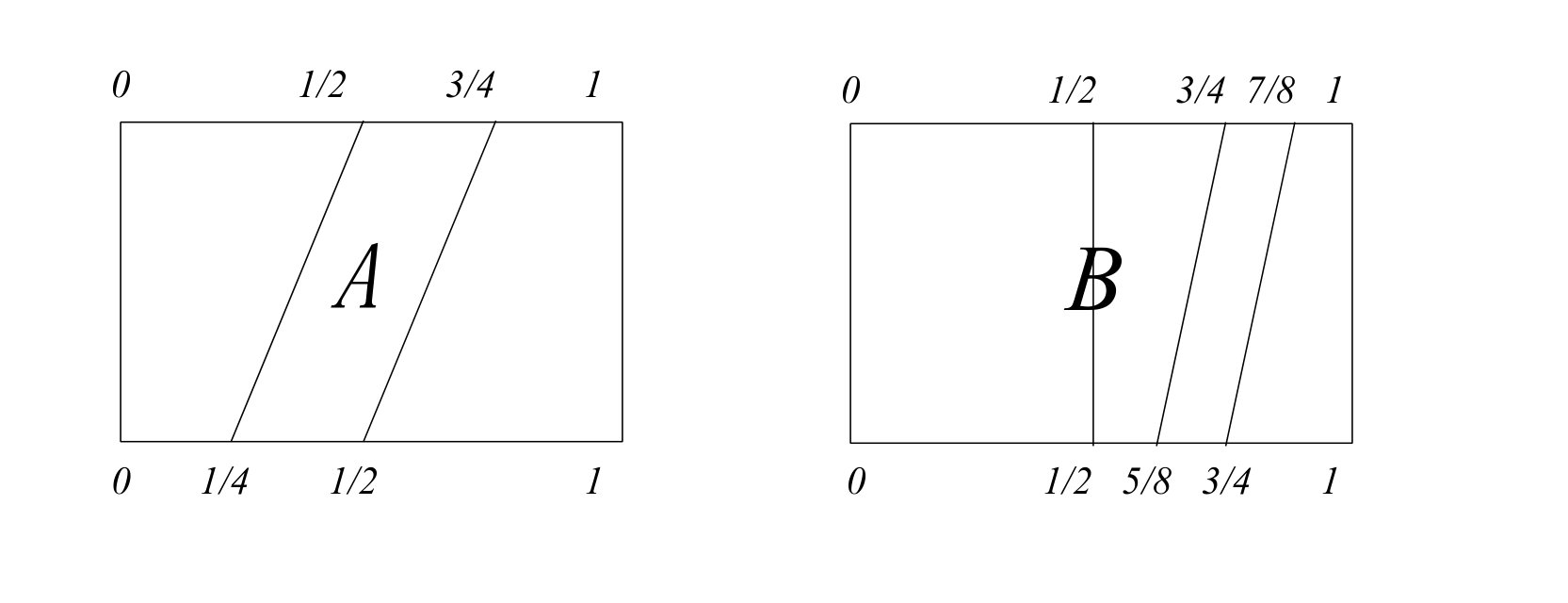 Figure 1
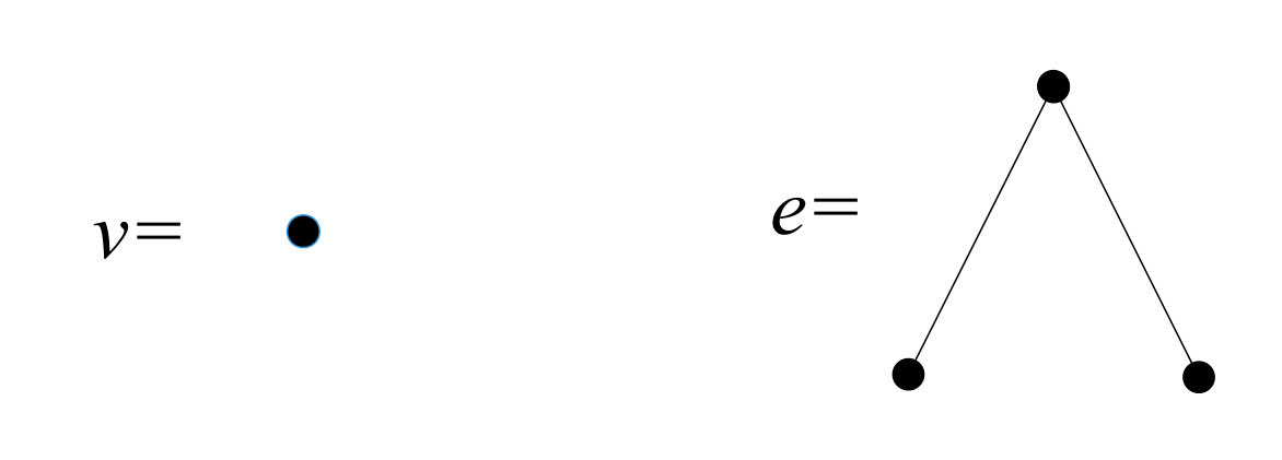 Figure 2
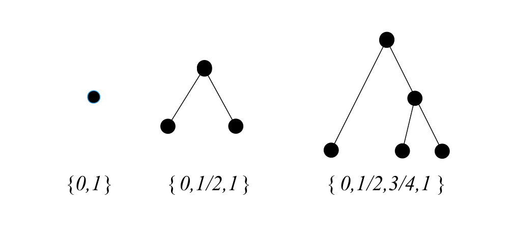 Figure 3
 Figure 4
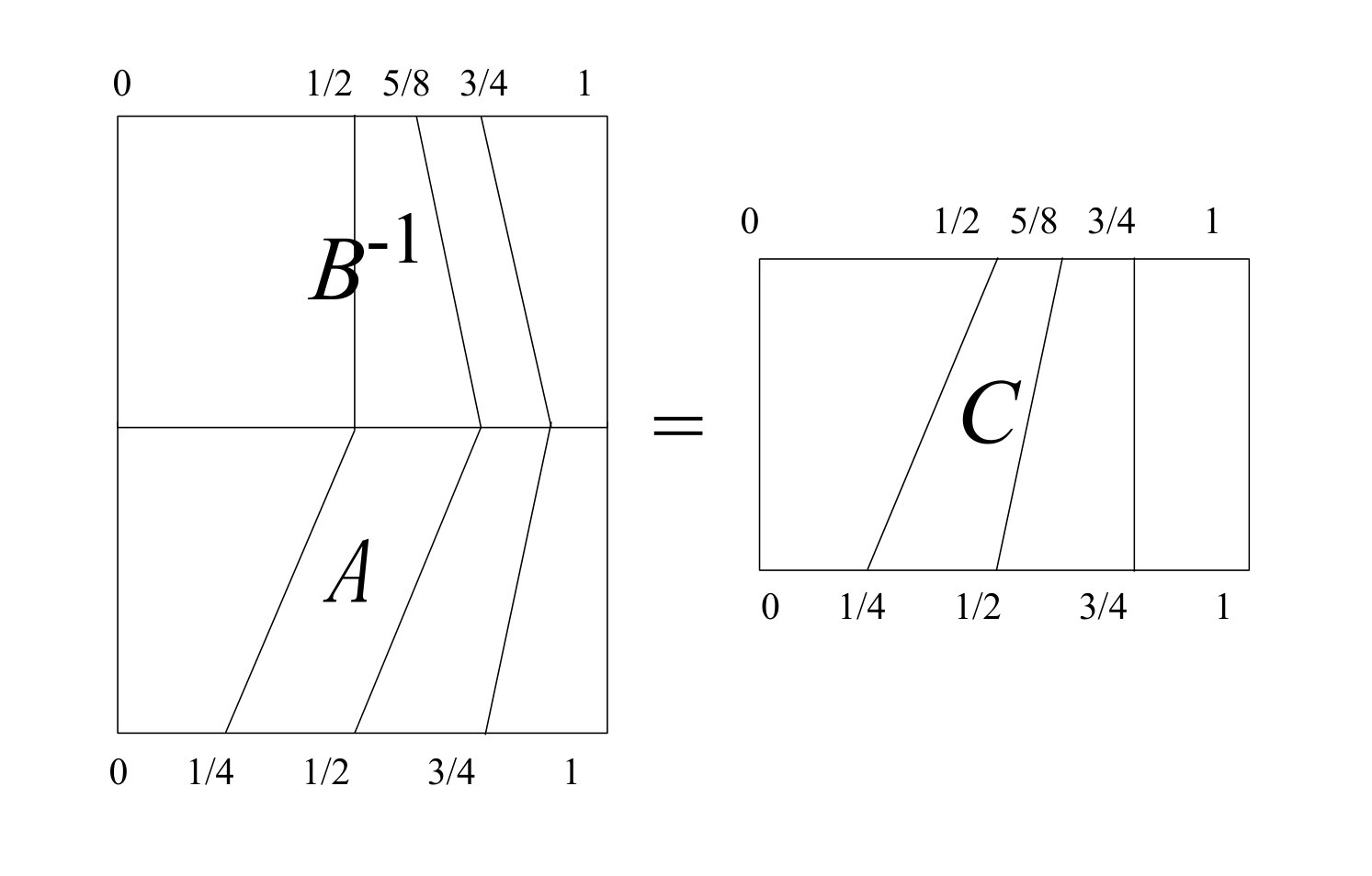 Figure 5
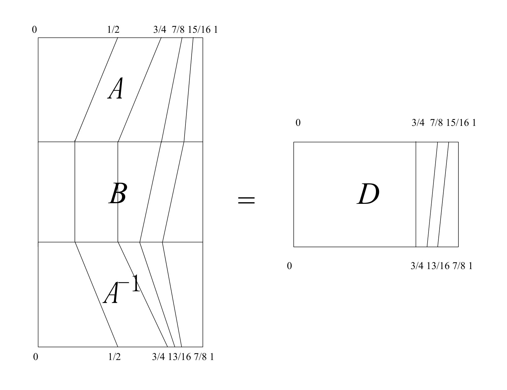 Figure 6