Better Software Analytics via "DUO": Data Mining Algorithms Using/Used-by Optimizers
Amritanshu Agrawal, Tim Menzies, Leandro L. Minku, Markus Wagner, Zhe, Yu

TL;DR
This paper introduces DUO, a novel approach combining data mining algorithms with optimizers to enhance empirical software engineering studies, enabling better models and more reliable results.
Contribution
It proposes a new integrated framework called DUO that leverages both data mining and optimization techniques for improved software analytics.
Findings
Optimizers can significantly improve data mining model performance.
Using DUO leads to faster and more accurate predictive models.
Unoptimized data miners can produce results that are easily refuted without optimization.
Abstract
This paper claims that a new field of empirical software engineering research and practice is emerging: data mining using/used-by optimizers for empirical studies or DUO. For example, data miners can generate models that are explored by optimizers. Also, optimizers can advise how to best adjust the control parameters of a data miner. This combined approach acts like an agent leaning over the shoulder of an analyst that advises "ask this question next" or "ignore that problem, it is not relevant to your goals". Further, those agents can help us build "better" predictive models, where "better" can be either greater predictive accuracy or faster modeling time (which, in turn, enables the exploration of a wider range of options). We also caution that the era of papers that just use data miners is coming to an end. Results obtained from an unoptimized data miner can be quickly refuted, just…
Click any figure to enlarge with its caption.
 Figure 1
 Figure 2
 Figure 3
 Figure 4
 Figure 5
 Figure 6
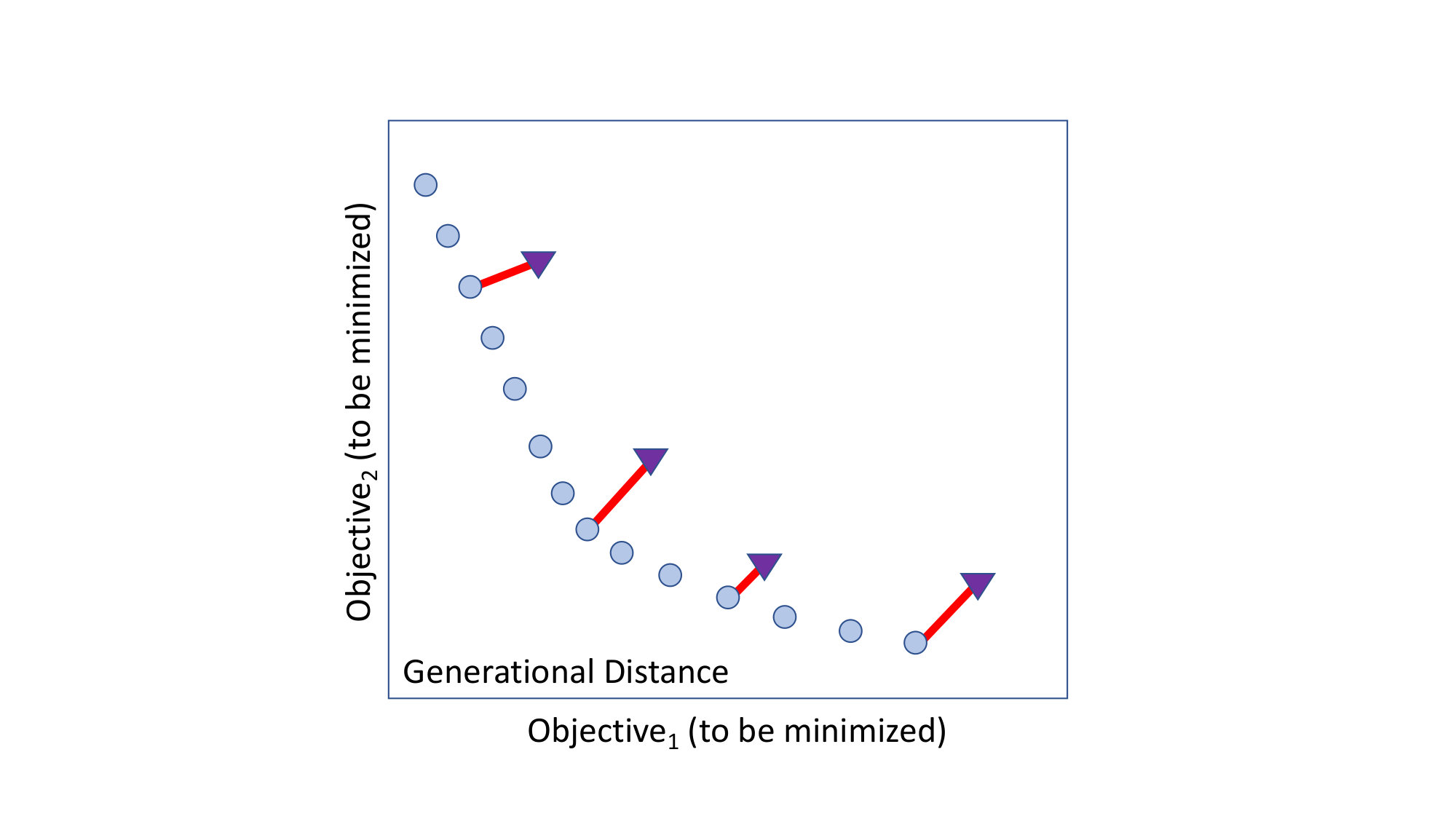 Figure 191210
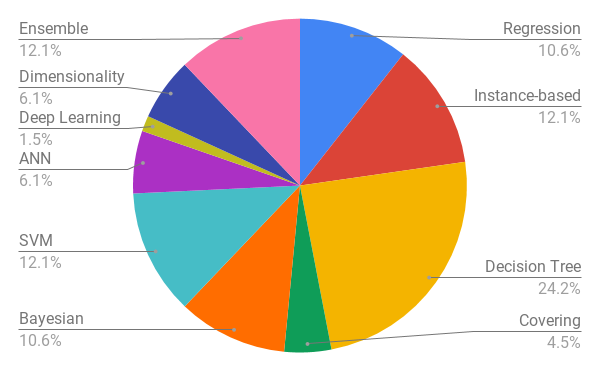 Figure 8
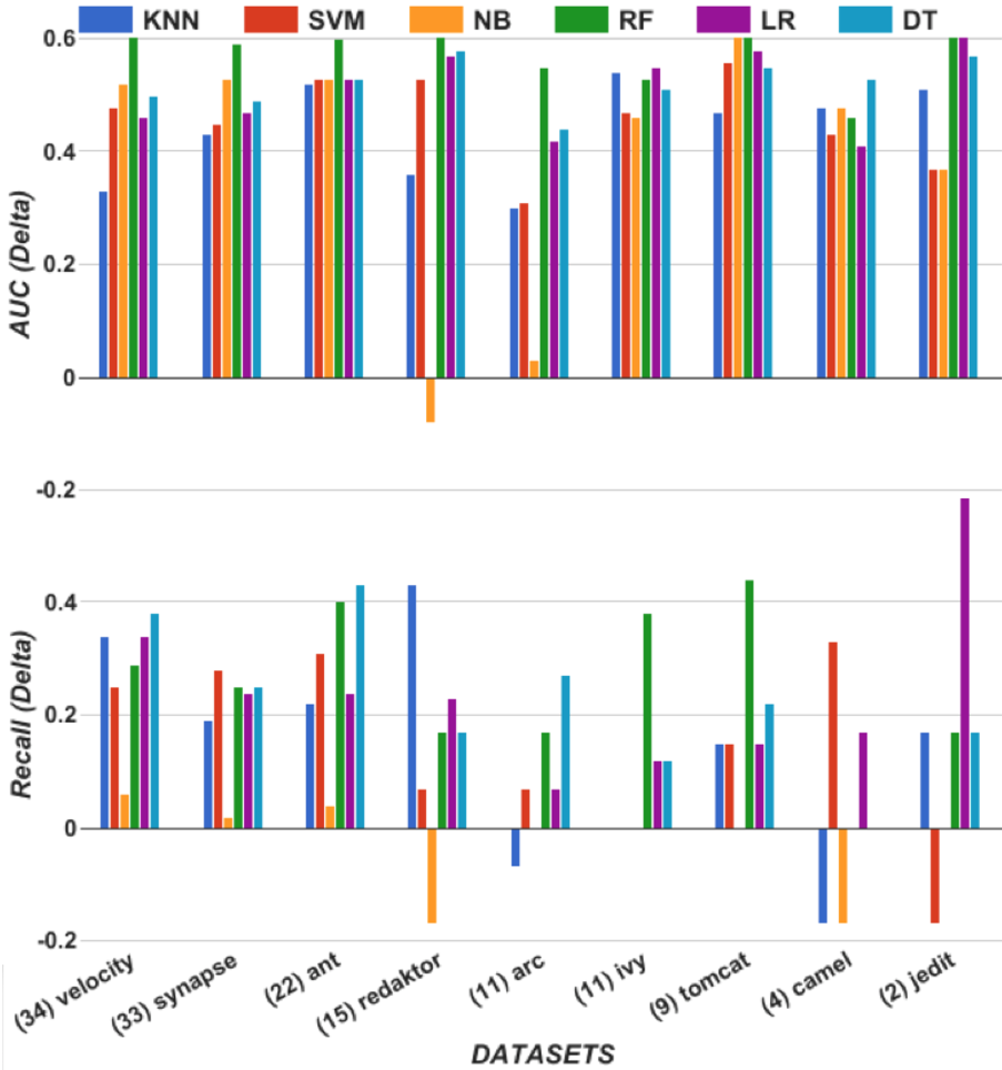 Figure 9
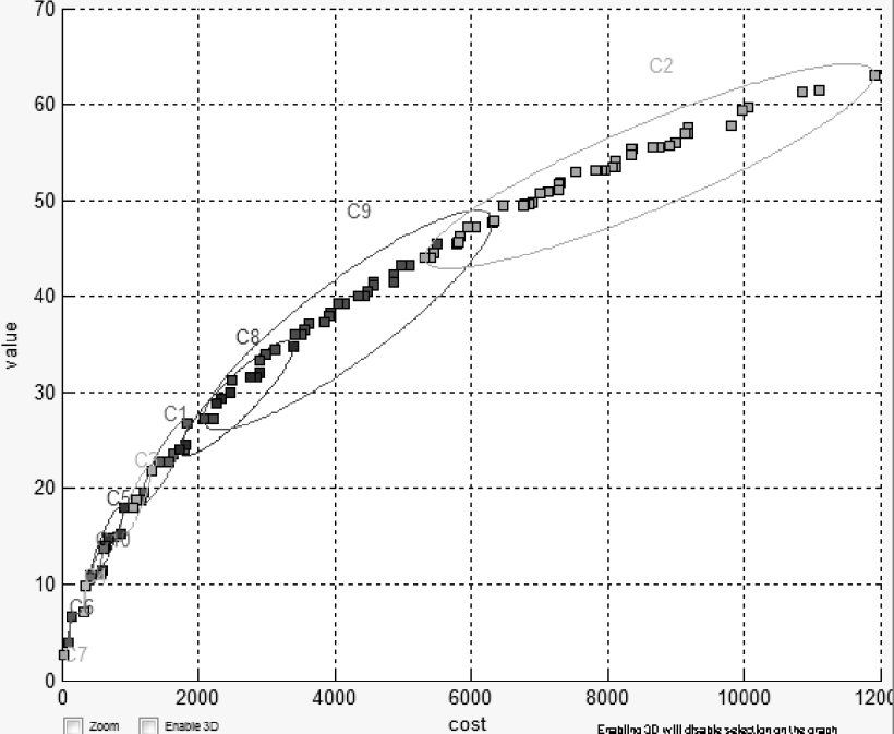 Figure 10
 Figure 11
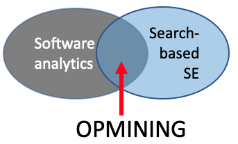 Figure 12
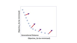 Figure 13
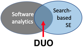 Figure 14
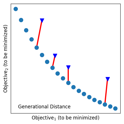 Figure 15
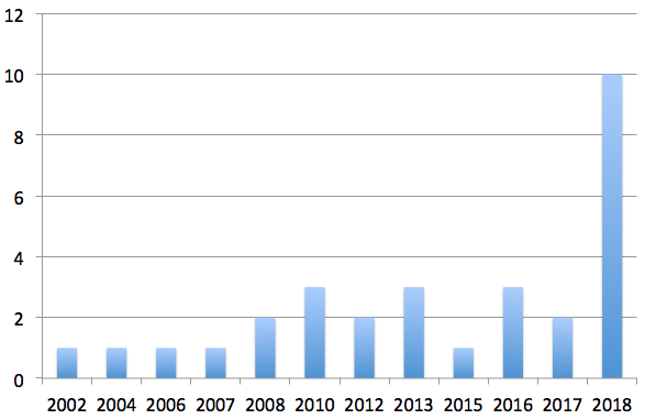 Figure 16
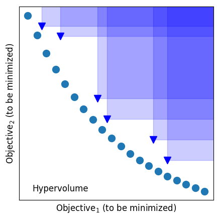 Figure 17
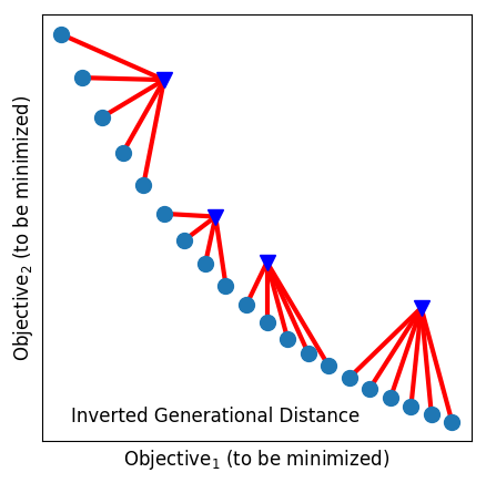 Figure 18
 Figure 19
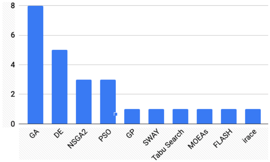 Figure 20
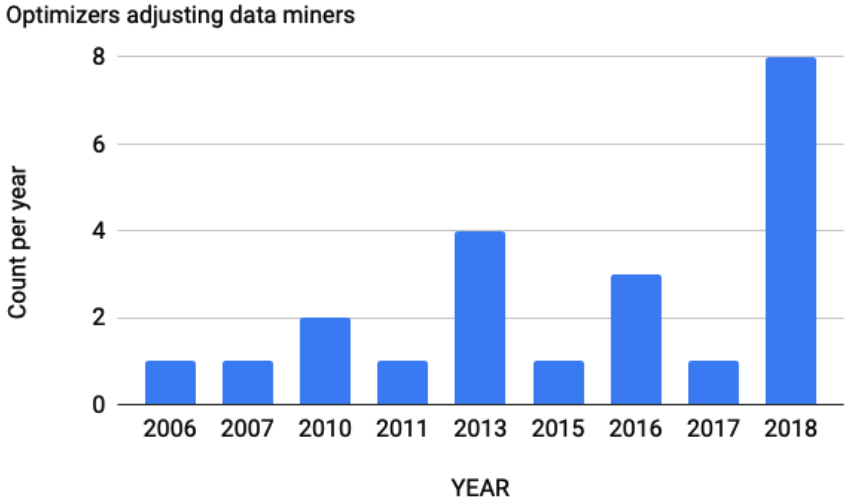 Figure 21
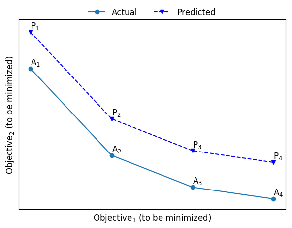 Figure 22
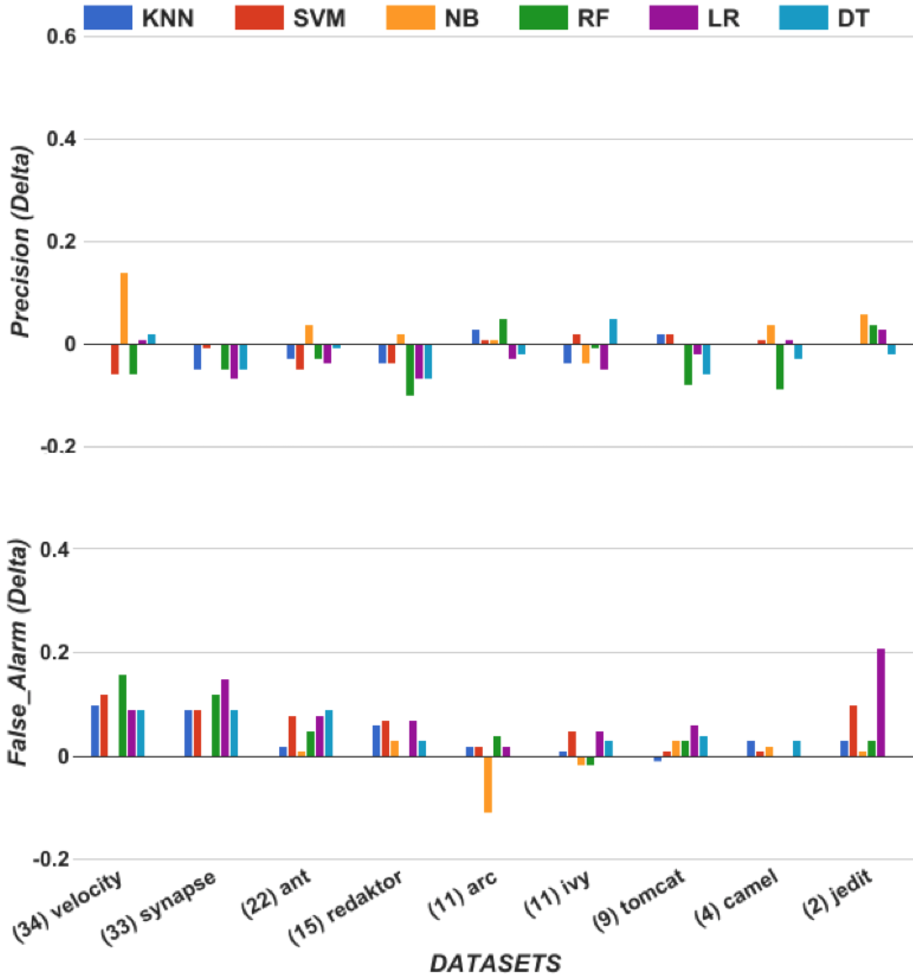 Figure 23
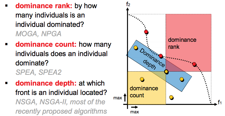 Figure 24
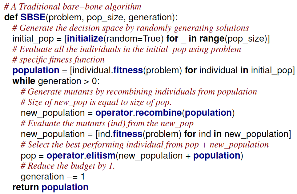 Figure 25
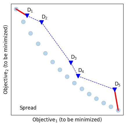 Figure 26
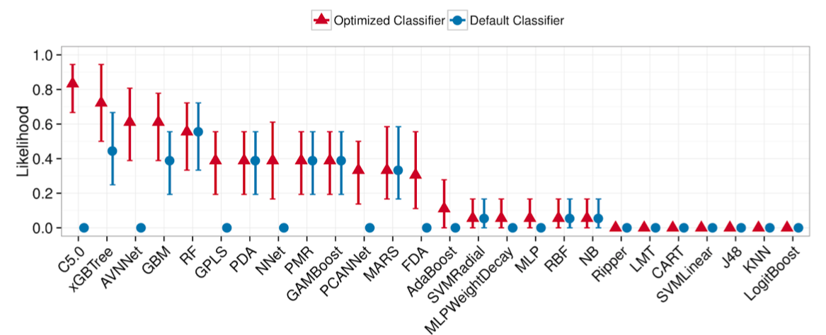 Figure 27
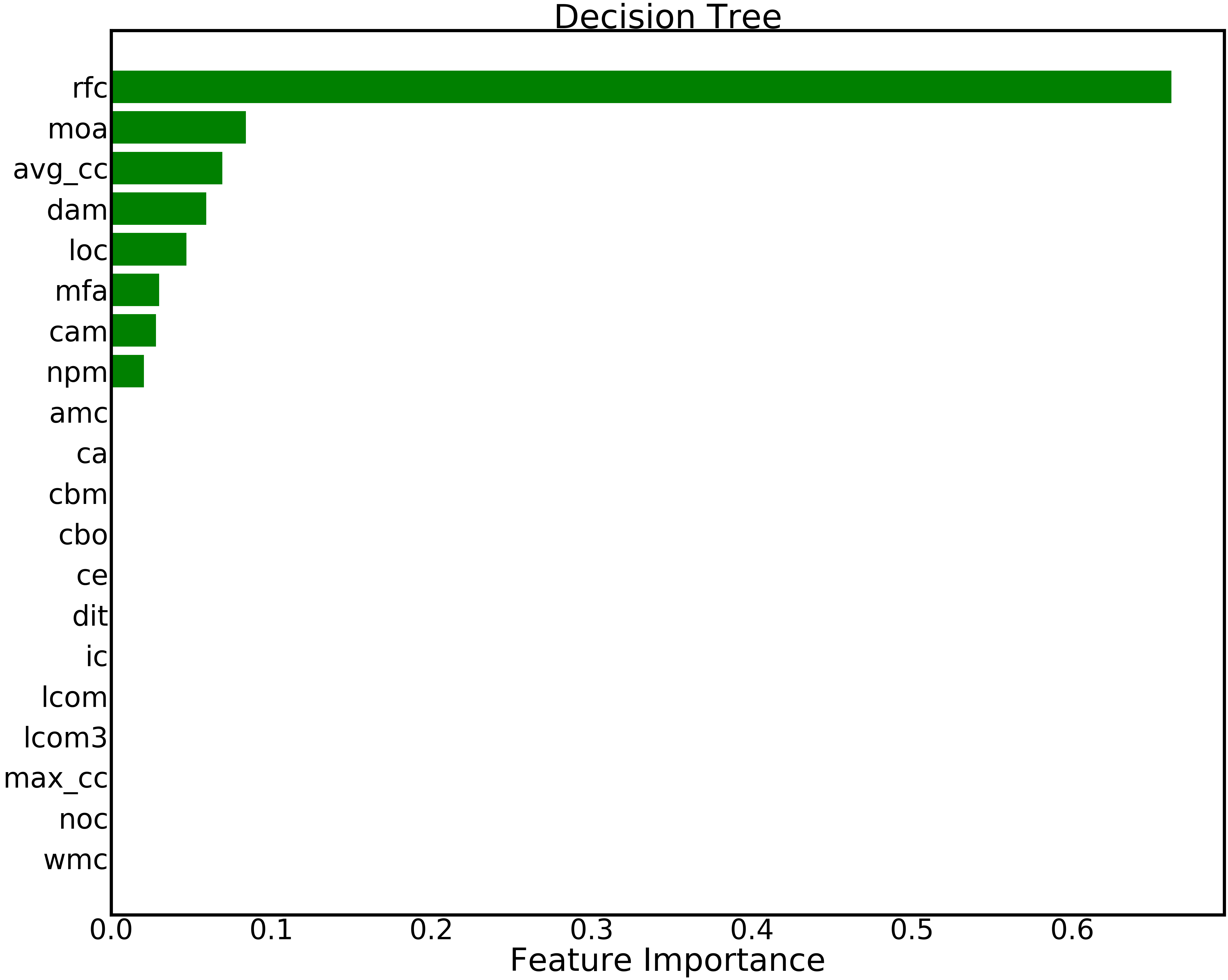 Figure 28
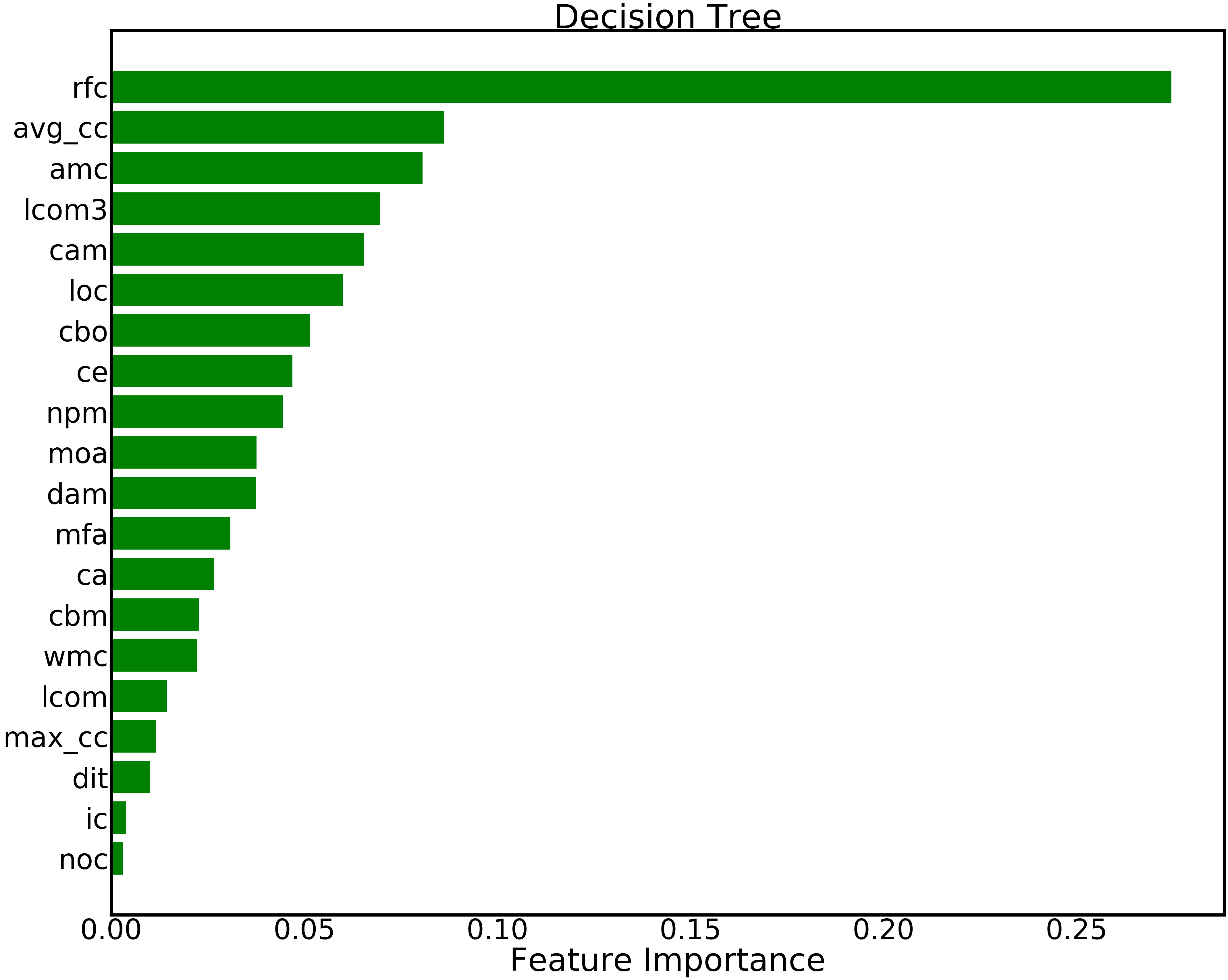 Figure 29
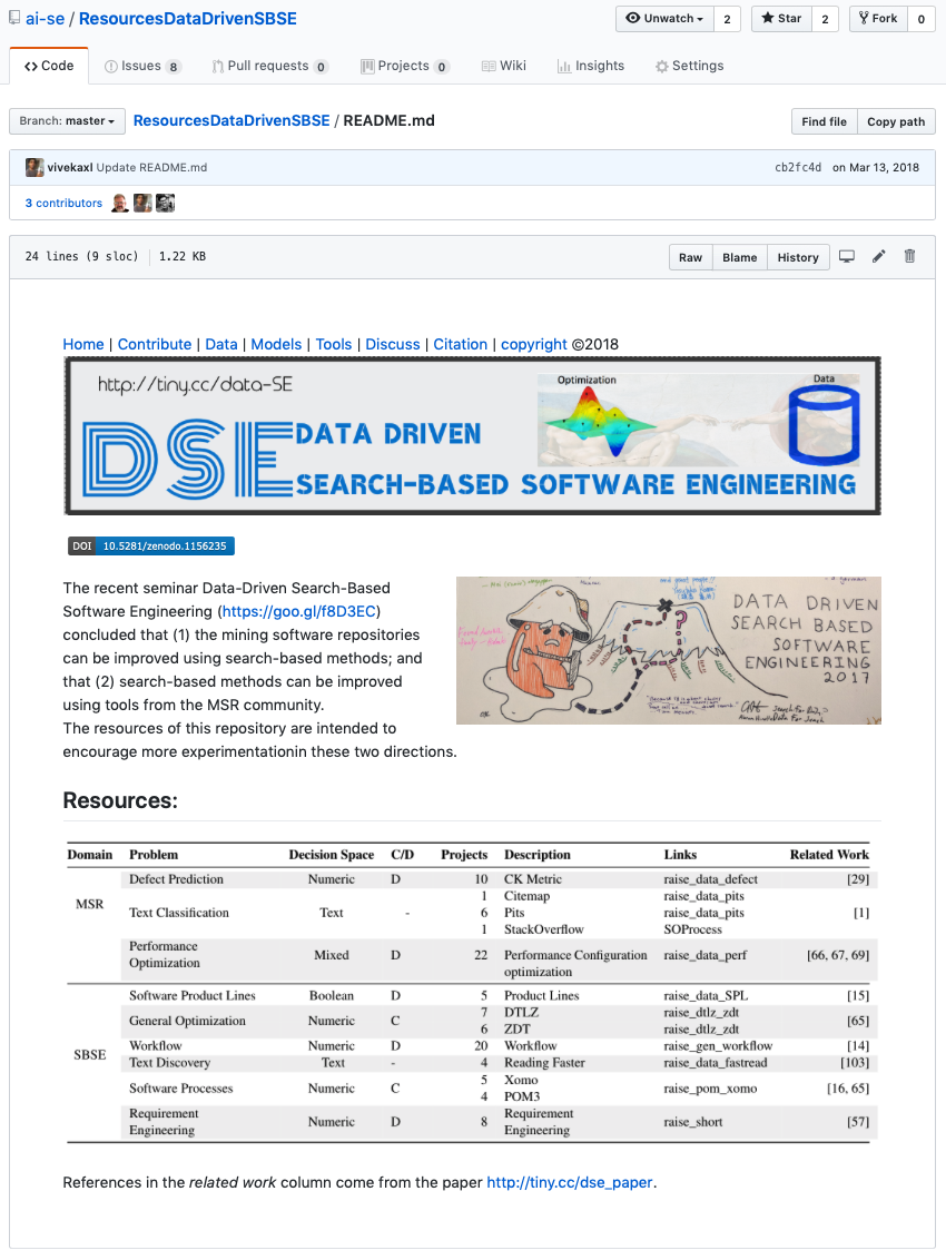 Figure 30
| Research | Q1. What papers have used DUO in the past? | |
|---|---|---|
| questions | Q2. When were they published? | |
| Q3. What problems from what software engineering domains have they tackled? | ||
| Q4. What optimizers have they used? | ||
| Q5. What data miners have they used? | ||
| Q6. What were the advantages offered by DUO? | ||
| Search | software engineering AND (“optimization” OR “evolutionary algorithm”) AND | |
| query | ( “data mining” OR “analytics” OR “machine learning”) | |
| Search | Three widely used literature sources were adopted: | |
| engines | • ACM Guide to Computing Literature (https://dl.acm.org/advsearch.cfm?coll=DL&dl=ACM) • IEEEXplore (https://ieeexplore.ieee.org/search/advsearch.jsp) • Google Scholar (https://scholar.google.com/#d=gs_asd&p=&u=) | |
| Inclusion | • ACM and IEEEXplore: 3 citations per year OR published in 2017/2018. | |
| criteria | • Google Scholar: (10 cites/year OR published in 2017/2018) AND in first 20 result pages. • For all search engines: paper relates to software engineering and must use DUO. | |
| The number of citations was more strict in Google Scholar, because this search engine usually retrieves more citations than the others. We restricted the Google Scholar results to the first 20 pages (200 papers) because Google Scholar allows papers that do not match the search query completely to be retrieved, resulting in 28,000 results that would need to be manually filtered for the software engineering domain and number of citations per year. | ||
| Q1 | The search query retrieved 393 results when considering all ACM, IEEEXplore and the first 20 pages of Google Scholar results. After excluding papers that did not match the citation and year of publication criteria, we obtained 90 papers. After excluding any duplicates and papers that were not in the software engineering domain, we obtained 72 papers. Finally, among these 72, 29 used DUO. These are: 1ali2018 ; 2sadiq2018 ; 13huang2006 ; 14zhong2004 ; 19kumar2008 ; 20huang2008 ; 26chiu2007 ; 31chen2018 ; 35fu2016 ; 38minku2013 ; 40sarro2016 ; 42oliveira2010ga ; 43panichella2013effectively ; 44liu2010evolutionary ; 54agrawal2018better ; 55de2010symbolic ; 57agrawal2018wrong ; 60fu2017easy ; 64abdessalem18 ; 87nair2017using ; 88majumder2018500+ ; 89chen2018sampling ; 90nair2018finding ; 93du2015evolutionary ; 94minku2013analysis ; 97sarro2012further ; 98sarro2012single ; 100feather2002converging ; 102treude2018per . In addition, we found a literature review related to DUO 30afzal2011 . This review is on the topic of genetic programming for predictive modeling in software engineering. Genetic programming can be seen as an optimization algorithm. | |
| Q2 | The number of DUO papers published per year is shown below, with 2018 having the largest number of papers. One might claim that this is because we ignore the number of citations in 2018. However, this is also the case for 2017, which had a considerably smaller number of DUO papers. Therefore, DUO seems to have been recently attracting increased research interest. | |
| 2002 1 2004 1 2006 1 2007 1 2008 2 2010 3 2012 2 2013 3 2015 1 2016 2 2017 2 2018 10 | ||
| Q3 | Domain where DUO is applied: | Specific problem: |
| Project management | Software effort estimation 13huang2006 ; 19kumar2008 ; 20huang2008 ; 26chiu2007 ; 38minku2013 ; 40sarro2016 ; 42oliveira2010ga ; 94minku2013analysis ; 98sarro2012single ; 89chen2018sampling , managing human resources 31chen2018 . | |
| Requirements | Requirements optimization 100feather2002converging . | |
| Design | Software architecture optimization 93du2015evolutionary , extraction of products from very large product lines 89chen2018sampling . | |
| Security | Intrusion detection1ali2018 ; 2sadiq2018 | |
| Software quality | Software detect prediction 14zhong2004 ; 35fu2016 ; 44liu2010evolutionary ; 54agrawal2018better ; 55de2010symbolic ; 97sarro2012further ; 47tantithamthavorn2016automated , test case generation 64abdessalem18 . | |
| Software configuration | Software configuration optimization 90nair2018finding ; 87nair2017using ; 31chen2018 . | |
| Text mining: StackOverflow | Linking posts 60fu2017easy ; 57agrawal2018wrong , topic modeling 57agrawal2018wrong ; 102treude2018per . | |
| Text mining: Defect Reports | Defect reports topic modeling 57agrawal2018wrong . | |
| Text mining: Software Artifact Search, Linking and Labeling | Traceability link recovery 43panichella2013effectively , locate features in source code 43panichella2013effectively , software artifacts labeling 43panichella2013effectively , topic modeling of software engineering papers 57agrawal2018wrong , Stack Overflow/GitHub topic modeling 102treude2018per . | |
| Q4 | See Table 2. | |
| Q5 | See Table 3. | |
| Q6 | See Sections 4, 5 and 6. | |
| Genetic Algorithms (GAs) execute over multiple generations. Generation zero is usually initialized at random. After that, in each generation, candidate items are subject to select (prune away the less interesting solutions), crossover (build new items by combining parts of selected items), and mutate (randomly perturb part of the new solutions). Modern GAs take different approaches to the select operator e.g. dominance rank, dominance count, and dominance depth. Notable exceptions are MOEA/D that use a decomposition operator to divide all the solutions into many small neighborhoods where if anyone finds a better solution, all its neighbors move there as well anderson2005practical ; 13huang2006 ; 26chiu2007 ; 40sarro2016 ; 42oliveira2010ga ; 43panichella2013effectively ; 93du2015evolutionary ; 94minku2013analysis ; 97sarro2012further . |
| Different evolution (DE) execute over multiple generations. Generation zero is usually initialized at random. After that, in each generation, candidate items are subject to select (prune away the less interesting solutions), mutate (build new items by combining with 3 other random candidates from the same generation) Storn:1997 ; 35fu2016 ; 54agrawal2018better ; 57agrawal2018wrong ; 60fu2017easy ; 88majumder2018500+ . |
| MOEAs contains different types of multi-objective evolutionary algorithms such as MOEA/D, NSGA-II, and more. They differ based on either the diversity mechanism (such as crowding distance or hypervolume contribution), or their sorting algorithm, or their use of target vectors, etc.huang2005multiobjective ; 38minku2013 ; deb02 ; 31chen2018 ; 40sarro2016 ; 64abdessalem18 ; Chand2015manyemo . |
| Particle Swarm Optimization (PSO) works by having a swarm of candidates where these candidates move around in the search space using simple formulae. The movements of the particles are guided by their own best-known position in the search-space as well as the entire swarm’s best-known position. When improved positions are being discovered these will then come to guide the movements of the swarm poli2007particle ; 1ali2018 ; 2sadiq2018 ; 55de2010symbolic . |
| Genetic programs (GPs) are like GAs except that while GAs manipulate candidates that are lists of options, GPs manipulate items that are trees. GPs can, therefore, be better for problems with some recursive structure (e.g. learning the parse tree of a useful equation) or when human-readable models are sought banzhaf1998genetic ; koza1994genetic ; 30afzal2011 . |
| SWAY first randomly generates a large number of candidates, recursively divides the candidates and only selects one. SWAY quits after the initial generation while GA reasons over multiple generations. It makes no use of reproduction operators so there is no way for lessons learned to accumulate as it executes 31chen2018 . |
| Tabu Search uses a local or neighborhood search procedure to iteratively move from one potential solution x to an improved solution x’ in the neighborhood of x, until some stopping criterion has been satisfied glover1998tabu ; 31chen2018 . |
| FLASH, a sequential model-based method such as Bayesian optimization, is a useful strategy to find extremes of an unknown objective. FLASH is efficient because of its ability to incorporate prior belief as already measured solutions (or configurations), to help direct further sampling. Here, the prior represents the already known areas of the search (or performance optimization) problem. The prior can be used to estimate the rest of the points (or unevaluated configurations). Once one (or many) points are evaluated based on the prior, the posterior can be defined. The posterior captures the updated belief in the objective function. This step is performed by using a machine learning model, also called surrogate model 90nair2018finding . |
| Genetic Algorithm 31% MOEAs 15% Differential Evolution 20% Particle Swarm Optimization 12% Genetic Programming 7% Tabu Search 4% SWAY 7% Flash 4% |
| Decision Tree learners such as CART and C4.5 seek attributes which, if we split on their ranges, most reduces the expected value of the diversity in splits. These algorithms then recurse over each split to find further useful divisions. For numeric classes, diversity may be measured in terms of variance. For discrete classes, the Gini or entropy measures can assess diversity. Decision tree learners are widely applied in software engineering due to the simplicity and interpretability 22catal2009 ; 24vandecruys2008 ; 26chiu2007 ; 35fu2016 ; 40sarro2016 ; 42oliveira2010ga ; 44liu2010evolutionary ; 47tantithamthavorn2016automated ; 54agrawal2018better ; 55de2010symbolic ; 64abdessalem18 ; 87nair2017using ; 90nair2018finding ; 94minku2013analysis . |
| Support Vector Machines (SVMs) are supervised learning trying to separate training items from two classes by a clear gap steinwart2008support . For linearly non-separable problems, SVMs either allow but penalize misclassification of training items (soft-margin) or utilize kernel tricks to map input data to a higher-dimensional feature space before learning a hyperplane to separate the two classes. Many software engineering researchers have explored using SVM models to predict software artifacts 24vandecruys2008 ; 42oliveira2010ga ; 47tantithamthavorn2016automated ; 54agrawal2018better ; 55de2010symbolic ; 60fu2017easy ; 88majumder2018500+ ; 97sarro2012further . |
| Instance-based algorithms: instead of fitting a model on the training data, instance-based algorithms stores all the training data as a database. When a new test item comes, the similarities between the test item and every training item are measured. The test item is then classified to the class where most of its similar training items belong to. Examples of instance-based algorithms include k-nearest neighbor 24vandecruys2008 ; 40sarro2016 ; 47tantithamthavorn2016automated ; 54agrawal2018better and analogy algorithms 13huang2006 ; 26chiu2007 ; 94minku2013analysis ; 40sarro2016 . |
| Ensemble algorithms use multiple learning algorithms to obtain better predictive performance than could be obtained from any of the constituent learning algorithms alone polikar2006ensemble . Usually, an ensemble algorithm builds multiple weak models that are independently trained and combines the output of each weak model in some way to make the overall prediction. Examples of ensemble algorithms include boosting freund1996experiments ; 47tantithamthavorn2016automated , bagging breiman1996bagging ; 47tantithamthavorn2016automated ; 94minku2013analysis , and random forest liaw2002classification ; 22catal2009 ; 35fu2016 ; 54agrawal2018better ; 102treude2018per . |
| Bayesian algorithms collect separate statistics for each class. Those statistics are used to estimate the prior distribution and the likelihood of each item in each class. When classifying a new test item, the estimated prior distribution and likelihood are applied to calculate its posterior distribution, which is then used to predict the class of the test item. Bayesian algorithms are widely applied in solving classification problems in software engineering 1ali2018 ; 2sadiq2018 ; 22catal2009 ; 42oliveira2010ga ; 47tantithamthavorn2016automated ; 54agrawal2018better ; 55de2010symbolic . |
| Regression algorithms use predefined functions to model the mapping from input space to output space. Parameters of the predefined function are estimated by minimizing the error between the ground truth outputs and the function outputs. Regression algorithms can be applied to solve both regression (e.g. linear regression 40sarro2016 ) and classification problems (e.g. logistic regression 24vandecruys2008 ; 35fu2016 ; 47tantithamthavorn2016automated ; 54agrawal2018better ; 40sarro2016 ). |
| Artificial Neural Networks (ANNs) are models that are inspired by the structure and function of biological neural networks van2018artificial . An ANN is based on a collection of connected units or nodes called artificial neurons, which loosely model the neurons in a biological brain. Each connection, like the synapses in a biological brain, can transmit a signal from one artificial neuron to another. An artificial neuron that receives a signal can process it and then signal additional artificial neurons connected to it. Such ANNs are usually applied in software engineering as baseline algorithms 26chiu2007 ; 47tantithamthavorn2016automated ; 55de2010symbolic ; 94minku2013analysis . |
| Dimensionality reduction algorithms transform the data in the high-dimensional space to a space of fewer dimensions roweis2000nonlinear . The resulting low-dimensional space can be used as features to train other data mining models or directly used as a clustering result. Examples of dimensionality reduction algorithms include principal component analysis jolliffe2011principal , linear discriminant analysis riffenburgh1957linear ; 47tantithamthavorn2016automated , and latent Dirichlet allocation blei2003latent ; 43panichella2013effectively ; 57agrawal2018wrong ; 102treude2018per . |
| Covering (rule-based) algorithms provide mechanisms that generate rules in a bottom-up, separate-and-conquer manner by concentrating on a specific class at a time and maximizing the probability of the desired classification. Examples of rule-based algorithms include PRISM kwiatkowska2011prism and RIPPER cohen1995fast ; 24vandecruys2008 ; 47tantithamthavorn2016automated ; 55de2010symbolic . |
| Deep Learning methods are a modern update to ANNs that exploit abundant cheap computation. Deep learning uses a cascade of multiple layers of nonlinear processing units for feature extraction and transformation. Each successive layer uses the output from the previous layer as input. In a supervised or unsupervised manner, it learns multiple levels of representations that correspond to different levels of abstraction; the levels form a hierarchy of concepts deng2014deep . Examples of instance-based algorithms include deep belief networks and convolutional neural network 60fu2017easy . |
| Decision tree learners 24% Support Vector Machines 13% Instance-based algorithms 11% Ensemble algorithms 11% Bayesian algorithms 11% Regression algorithms 10% Artificial Neural Networks 7% Dimensionality reduction algorithms 7% Covering (rule-based) algorithms 5% Deep Learning 2% |
Peer Reviews
No public reviews on file for this paper yet. If you reviewed it on a platform where reviews are public (OpenReview, ICLR, NeurIPS, ICML), you can paste yours below so the community can read it here.
Videos
No videos yet. Explain this paper in a talk, walkthrough, or lecture? Add one.
∎
11institutetext: Amritanshu Agrawal, Tim Menzies, Zhe Yu 22institutetext: Department of Computer Science, North Carolina State University, Raleigh, NC, USA. 22email: [email protected] 33institutetext: Leandro L. Minku 44institutetext: School of Computer Science, University of Birmingham, Edgbaston, Birmingham, UK. 44email: [email protected] 55institutetext: Markus Wagner 66institutetext: School of Computer Science, University of Adelaide, Adelaide, SA, Australia. 66email: [email protected]
Better Software Analytics via “DUO”:
Data Mining Algorithms Using/Used-by Optimizers
Amritanshu Agrawal
Tim Menzies
Leandro L. Minku
Markus Wagner
Zhe Yu Authors listed alphabetically.
Abstract
This paper claims that a new field of empirical software engineering research and practice is emerging: data mining using/used-by optimizers for empirical studies, or DUO. For example, data miners can generate models that are explored by optimizers. Also, optimizers can advise how to best adjust the control parameters of a data miner. This combined approach acts like an agent leaning over the shoulder of an analyst that advises “ask this question next” or “ignore that problem, it is not relevant to your goals”. Further, those agents can help us build “better” predictive models, where “better” can be either greater predictive accuracy or faster modeling time (which, in turn, enables the exploration of a wider range of options). We also caution that the era of papers that just use data miners is coming to an end. Results obtained from an unoptimized data miner can be quickly refuted, just by applying an optimizer to produce a different (and better performing) model. Our conclusion, hence, is that for software analytics it is possible, useful and necessary to combine data mining and optimization using DUO.
Keywords:
Software analytics, data mining, optimization, evolutionary algorithms
1 Introduction
After collecting data about software projects, and before making conclusions about those projects, there is a middle step in empirical software engineering where the data is interpreted. When the data is very large and/or is expressed in terms of some complex model of software projects, then interpretation is often accomplished, in part, via some automatic algorithm. For example, an increasing number of empirical studies base their conclusions on data mining algorithms (e.g. see 27menzies2013 ; menzim18r ; bird2015art ; menzies2013data ; 2016tim ) or model-intensive algorithms such as optimizers (e.g. see the recent section on Search-Based Software Engineering in the December 2016 issue of this journal Kessentini16 ).
This paper asserts that, for software analytics it is possible, useful and necessary to combine data mining and optimization. We call this combination DUO, short for data miners using/used-by optimizers. Once data miners and optimizers are combined, this results in a very different and interesting class of interpretation methods for empirical SE data. DUO acts like an agent leaning over the shoulder of an analyst that advises “ask this question next” or “ignore that problem, it is not relevant to your goals”. Further, DUO helps us build “better” predictive models, where “better” can be for instance greater predictive accuracy, or models that generalize better, or faster modeling time (which, in turn, enables the faster exploration of a wider range of options). Therefore, DUO can speed up and produce more reliable analyses in empirical studies.
This paper makes the following claims about DUO:
- •
Claim1: For software engineering tasks, optimization and data mining are very similar. Hence, it is natural and simple to combine the two methods.
- •
Claim2: For software engineering tasks. optimizers can greatly improve data miners. A data miner’s default tuners can lead to sub-optimal performance. Automatic optimizers can find tunings that dramatically improve that performance 35fu2016 ; 54agrawal2018better ; 57agrawal2018wrong .
- •
Claim3: For software engineering tasks, data miners can greatly improve optimization. If a data miner groups together related items, an optimizer can explore and report conclusions that are general across a set of solutions. Further, optimization for SE problems can be very slow (e.g. consider the 15 years of CPU needed by Wang et al. wang2013searching ). But if that optimization executes over the groupings found by a data miner, that inference can terminate orders of magnitude faster 90nair2018finding ; krall2015gale .
- •
Claim4: For software engineering tasks, data mining without optimization is not recommended. Conclusions reached from an unoptimized data miner can be changed, sometimes even dramatically improved, by running the same tuned learner on the same data 35fu2016 . Researchers in data mining should, therefore, consider adding an optimization step to their analysis.
This paper extends a prior conference paper on the same topic Nair:2018 . That prior paper focused on case study material for DUO-like applications (see Figure 1). While a useful resource, it did not place DUO in a broader context. Nor did it contain the literature review of this paper. That is, this paper is both more general (discussing the broader context) and more specific (containing a detailed literature review) than prior work.
The rest of this paper is organized as follows. The next section describes some related work. After that, we devote one section to each of Claim1, Claim2, Claim3 and Claim4. To defend these claims we use evidence drawn from a literature review of applications of DUO, described in Table 1 (Table 2 and Table 3 offer notes on the data miners and optimizers seen in the literature review). Finally, a Research Directions section discusses numerous open research issues that could be better explored within the context of DUO.
2 Tutorial
Before discussing combinations of data miners and optimizers, we should start by defining each term separately, and discussing their relationship. Optimizers reflect over a model to learn inputs that most improve model output. Data miners, on the other hand, reflect over data to return a summary of that data. Data miners usually explore a fixed set of data while optimizers can generate more data by re-running the model times using different inputs. Data miners “slice” data such that similar patterns are found within each division. Optimizers “zoom” into interesting regions of the data, using a model to fill in missing details about those regions.
There are many different kinds of data miners, each of which might produce a different kind of model. For example, regression methods generate equations; nearest-neighbor-based methods might yield a small set of most interesting attributes and examples; and neural net methods return a weighted directed graph. Some data miners generate combinations of models. For example, the M5 “model tree learner” returns a set of equations and a tree that decides when to use each equation Quinlan92learningwith .
Whereas data miners usually have “hard-wired goals” (e.g. improve accuracy), the goals of an optimizer can be adjusted from problem to problem. In this way, an optimizer can be tuned to the needs of different business users. For example:
- •
For requirements engineers, we can find the least cost mitigations that enable the delivery of most requirements 100feather2002converging .
- •
For project managers, we can apply optimizers to software process models to find options that deliver more code in less time with fewer bugs Menzies:2007 .
- •
For developers, our optimizers can tune data miners looking for ways to find more bugs in fewer lines of code (thereby reducing the human inspection effort required once the learner has finished Fu2016Tuning .
- •
Etc.
In any engineering discipline, including software engineering, it is common to trade-off between multiple completing goals (e.g. all the examples in the above list are competing for multi-objective goals). Hence, for the rest of this tutorial section, we focus on multi-objective optimization.
2.1 Multi-Objective Optimization
All the optimizers of Table 2 seek the maxima or minima of an objective functions , (where are the objective or “evaluation” functions, is the number of objectives, is called the independent variable, and are the dependent variables).
For single-objective () problems, algorithms aim at finding a single solution able to optimize the objective function, i.e., a global maximum/minimum.
For multi-objective () problems, there is no single ‘best’ solution, but a number of ‘best’ solutions. These best solutions, also known as the Pareto Front, are the non-dominated solutions found using a dominance relation. This domination criterion can be defined many ways:
- •
The standard “Boolean dominance” predicates says that dominates another , if is better than in at least one objective and if is no worse than in all other objectives.
- •
Another style of domination predicate is the “Zitler indicator” shown in Algorithm 1. This method reports what loses least: moving from to or to (and the solution is preferred if moving to results is the least loss; see Algorithm 1).
- •
Regardless of how domination is defined, a solution is called non-dominated if no other solution dominates it.
As shown in Figure 2, solutions found by an optimization algorithm are called the Predicted Pareto Front (PF). The list of best solutions of a space found so far is known as the Actual Pareto Front. As this can be unknowable in practice or prohibitively expensive to generate, it is common to build the actual front using the union of all optimization outcomes all non-dominated solutions.
2.2 Meta-heuristic Optimizers
Any non-trivial software system contains thousands to millions of condition statements (if, case, etc). Each of these conditions sub-divides the internal state space of a software system. From a technical perspective, this means that the state space of software is not a continuous function (since each conditional creates a different sub-system with different properties). Accordingly, to optimize a software system, simplistic numeric optimizers are not appropriate. Instead, a common approach is to use the search-based meta-heuristic methods shown in Figure 3. The rest of this section offers notes on that pseudo-code.
Multi-objective optimizers for SE use either a model (which represent a software process boehm1995cost ) or can be directly applied to any software engineering system (including problems that require evaluating a solution by running a specific benchmark krall2015gale ). However the model or software system is created, it can be represented in the decision space in a myriad of ways, for example, as Boolean or numerical vectors, as strings, and as graphs. (and the space of all solutions that can be represented in this way is the decision space).
Search-based meta-heuristic methods explore and refine a population of candidate solutions using the decision space representation. The process of search typically starts by creating a population of random solutions (valid or invalid) saber2017seeding ; chen2017beyond ; 89chen2018sampling ; henard2015combining . A fitness function then maps the solution (which is represented using numerics) to a numeric scale (also known as Objective Space) which is used to distinguish between good and not so good solutions Simply put, the fitness function is a transformation function which converts a point in the decision space to the objective space.
Some variation operator is then applied to mutate the solutions (that is, to generate new candidate solutions). Typically, unary operators are called mutation operators, and operators with higher arity are called crossover operators.
Then, it is common to use operators that apply some pressure towards selecting better solutions from the union of the current population and the newly created solutions. This selection is done either deterministically (e.g., elitism operator) or stochastically. An important class of operator is *Elitism * which simulates the ‘survival of the fittest’ strategy, i.e., it eliminates not so good solutions thereby preserving the good solutions in the population.
As shown by the while loop of Figure 3, a meta-heuristic algorithm iteratively improves the population (set of solutions) as, at each iteration, each member of the population might be mutated or eliminated via elitism. Each step of this process, which includes generation of new solutions using recombination of the existing population and selecting solutions using the elitism operator, is called a generation. Over successive generations, the population ‘evolves’ (in the best case) toward a globally optimal solution.
2.3 How is it all assessed?
For single-objective problems, measures such as absolute residual or rank-difference can be very useful. For multi-objective problems, the evaluation scores must explore trade-offs between (potentially) competing goals. Figure 4 illustrates some of the standard evaluation measures used for multi-objective reasoning. The rest of this section explains that figure.
Generational distance is the measure of convergence—how close is the predicted Pareto front to the actual Pareto front. It is defined to measure (using Euclidean distance) how far are the solutions that exist in the population from the nearest solutions in the Actual Pareto front . In an ideal case, the GD is 0, which means the predicted PF is a subset of the actual PF. Note that it ignores how well the solutions are spread out.
Spread is a measure of diversity—how well the solutions in are spread. An ideal case is when the solutions in is spread evenly across the Predicted Pareto Front.
Inverted Generational Distance measures both convergence as well as the diversity of the solutions—it measures the shortest distance from each solution in the Actual PF to the closest solution in Predicted PF. Like Generational distance, the distance is measured in Euclidean space. In an ideal case, IGD is 0, which means the Predicted PF is same as the Actual PF.
The Hypervolume indicator is used to measure both convergence as well as the diversity of the solutions—hypervolume is the union of the cuboids w.r.t. to a reference point. Note that the hypervolume implicitly defines an arbitrary aim of optimization. Also, it is not efficiently computable when the number of dimensions is large, however, approximations exist.
Lastly, we mention Approximation:. The Additive/multiplicative Approximation is an alternative measure which can be computed in linear time (w.r.t. to the number of objectives). It is the multi-objective extension of the concept of approximation encountered in theoretical computer science.
3 Claim1: For software engineering tasks, optimization and data mining are very similar
At first glance, the obvious connection between data miners and optimizers is that the former build models from data while the latter can be used to exercise those models (in order to find good choices within a model). Nevertheless, as far as we can tell, these two areas are currently being explored by different research teams. While counter-examples exist, data miners are used by software analytics workers and optimizers are used by researchers into search-based SE for the most part. As shown in Figure 5, the field we call “DUO” combines software engineering work from both fields.
Search-based software engineering harman2012search ; 5harman2001 characterizes SE tasks as optimizing for (potentially competing) goals; e.g. designing a product such that it delivers the most features at least cost 33sayyad2013 . Software analytics bird2015art ; 27menzies2013 ; menzim18r , on the other hand, is a workflow that distills large amounts of low-value data into small chunks of very high-value data. For example, software analytics might build a model predicting where defects might be found in source code 6gondra2008 .
For the most part, researchers in these two areas work separately (as witnessed by, say the annual Mining Software Repositories conference and the separate symposium on Search-based Software Engineering). What will be argued in this paper is that insights and methods from these two fields can be usefully combined. We say this because papers that combined data miners and optimizers explore important SE tasks:
- •
Project management 13huang2006 ; 19kumar2008 ; 20huang2008 ; 26chiu2007 ; 38minku2013 ; 40sarro2016 ; 42oliveira2010ga ; 94minku2013analysis ; 98sarro2012single ; 89chen2018sampling ; 31chen2018 ;
- •
Requirements engineering 100feather2002converging ;
- •
Software design 93du2015evolutionary ; 89chen2018sampling ;
- •
Software security 1ali2018 ; 2sadiq2018 ;
- •
Software quality 14zhong2004 ; 35fu2016 ; 44liu2010evolutionary ; 54agrawal2018better ; 55de2010symbolic ; 97sarro2012further ; 64abdessalem18 ; 47tantithamthavorn2016automated ;
- •
Software configuration 90nair2018finding ; 87nair2017using ; 31chen2018 ;
- •
Text mining of software-related textual artifacts 43panichella2013effectively ; 43panichella2013effectively ; 57agrawal2018wrong ; 102treude2018per .
In our literature review, we have seen four different flavors of this combined DUO approach:
- •
Mash-ups of data miners and optimizers: In this approach, data miners and optimizers can be seen as separate executables. For example, Abdessalem et al. 64abdessalem18 generate test cases for autonomous cars via a cyclic approach where an optimizer reflects on the output of data miners that reflect on the output of an optimizer (and so on).
- •
Data miners acting as optimizers: In this approach, there is no separation between the data miner and optimizer. For example, Chen et al. 89chen2018sampling show that their recursive descent bi-clustering algorithm (which is a data mining technique) outperforms traditional evolutionary algorithms for the purposes of optimizing SE models.
- •
Optimizers control the data miners: In this approach, the data miner is a subroutine called by the optimizer. For example, several recent papers improve predictive performance via optimizers that tune the control parameters of the data miner 35fu2016 ; 54agrawal2018better ; 47tantithamthavorn2016automated .
- •
Data miners control the optimizers: In this approach, the optimizer is a subroutine called by the data miner. For example, Majumder et al. 88majumder2018500+ use k-means clustering to divide up a complex text mining problem, then apply optimizers within each cluster. They report that this method speeds up their processing by up to three orders of magnitude.
To understand why data mining technology is so useful for optimization, and vice versa, we must dive deeper into the formal underpinnings of work in this area. Without loss of generality, an optimization problem is of the following format OptDef :
[TABLE]
where is the optimization variable of the problem,111This definition has been generalized with respect to OptDef , not to be restricted to continuous optimization problems, where are the objective functions (goals) to be minimized, are inequality constraints, and are equality constraints.222The optimization variable is usually identified by the symbol x, and the inequality and equality constraints are frequently identified by the symbols and in the optimization literature. However, we use the symbols a, and here to avoid confusion with the terminology used in data mining, which is introduced later in this section. Sometimes, there are no constraints (so and ). Also, we say a multi-objective problem has objectives, as opposed to a single-objective problem, where .
One obvious question about this general definition is “where do the functions come from?”. Traditionally, these have been built by hand but, as we shall see below, can be learned via data mining. That is, optimizers can explore the functions proposed by a learner.
An example of an optimization problem in the area of software engineering is to find a subset a of requirements that maximizes value if implemented333Any maximization problem can be re-written as a minimization problem., given a constrained budget , where Sagrado2011 . Many different algorithms exist to search for solutions to optimization problems. Table 2 shows the optimization algorithms that have been used by the software engineering community when applying DUO.
Data mining is a problem that involves finding an approximation of a function of the following format:
[TABLE]
where are the input variables, are the output variables of the function , X is the input space and Y is the output space. The input variables x are frequently referred to as the independent variables or input features, whereas y are referred to as the dependent variables or output features.
An example of a data mining problem in software engineering is software defect prediction hall2012systematic . Here, the input features could be a software component’s size and complexity, and the output feature could be a label identifying the component as defective or non-defective. Many different machine learning algorithms can be used for data mining. Table 3 shows data mining algorithms used by the software engineering community when applying DUO.
The functions and do not necessarily correspond to the optimization functions depicted in Eq. 1. However, the true function is unknown. Therefore, data mining frequently relies on machine learning algorithms to learn an approximation based on a set of known examples (data points) from . And, learning this approximation typically consists of searching for a function that minimizes the error (or other predictive performance metrics) on examples from . Therefore, learning such approximation is an optimization problem of the following format:
[TABLE]
where , and are the predictive performance metrics obtained by on . The functions depicted in Eq. 3 thus correspond to the functions depicted in Eq. 1. An example of performance metric function would be the mean squared error, defined as follows:
[TABLE]
As we can see from the above, solving a data mining problem means solving an optimization problem, i.e., optimization and data mining are very similar. Indeed, several popular machine learning algorithms are optimization algorithms. For example, gradient descent for training artificial neural networks, quadratic programming for training support vectors machines and least squares for training linear regression are optimization algorithms.
From the above, we can already see that optimization is of interest to data mining researchers, even though this connection between the two fields is not always made explicit in software engineering research. More explicit examples of how optimization is relevant to data mining in software engineering include the use of optimization algorithms to tune the parameters of the data mining algorithms, as mentioned at the beginning of this section and further explained in Sections 4 and 6. We consider such more explicitly posed connections between data mining and optimization as a form of DUO.
A typical distinction made between the optimization and data mining fields is data mining’s need for generalization. Despite the fact that data mining uses machine learning to search for approximations that minimize the error on a given dataset , the true intention behind data mining is to search for approximations that minimize the error on unseen data from , i.e., being able to generalize. As is unavailable for learning, data mining has to rely on a given known data set to find a good approximation . Several strategies can be adopted by machine learning to avoid poor generalization despite the unavailability of . For instance, the performance metric functions may use regularization terms Bishop , which encourage the parameters that compose to adopt small values, making less complex and thus generalize better. Another strategy is early stopping Bishop , where the learning process stops early, before finding an optimal solution that minimizes the error on the whole set .
However, even the distinction above starts to become blurry when considering that generalization can also frequently be of interest to optimization researchers. For example, in software configuration optimization (Section 5), the true optimization functions are often too expensive to compute, requiring machine learning algorithms to learn approximations of such functions. Optimization functions approximated by machine learning algorithms are referred to as surrogate models, and correspond to the approximation of Eq. 3. These approximation functions are then the one optimized, rather than the true underlying optimization function. Even though an optimization algorithm to solve this problem does not attempt to generalize, a data mining technique can do so on its behalf. We consider this as another form of DUO. Sections 4 and 5 explain how several other examples of software engineering problems are indeed both optimization and data mining problems at the same time, and how different forms of DUO can help solving these problems.
Overall, this section shows that optimization and data mining are very similar to each other, and that the typical distinction made between them can become very blurry when considering real world problems. Several software engineering problems require both optimization and generalization at the same time. Therefore, many of the ideas independently developed by the field of optimization are applicable to improve the field of data mining, and vice-versa. Sections 4 to 6 explain how useful DUO can and could be.
4 Claim2: For software engineering tasks, optimizers can greatly improve data miners
One of the most frequent ways to integrate data mining and optimization is via hyperparameter optimization. This is the art of tuning the parameters that control the choices within a data miner. While these can be set manually444Using a process called “engineering judgement”; i.e. guessing. we found that several papers in our literature review used optimizers to automatically find the best parameters 54agrawal2018better ; 35fu2016 ; 44liu2010evolutionary ; 97sarro2012further ; 14zhong2004 ; 102treude2018per ; 42oliveira2010ga . There are many reasons why this is so:
- •
These control parameters are many and varied. Even supposedly simple algorithms come with a daunting number of options. For example, the scitkit-learn toolkit lists over a dozen configuration options for Logistic Regression555 https://scikit-learn.org/stable/modules/generated/sklearn.linear_model.LogisticRegressionCV.html, accessed 30 November 2018.. This is an important point since recent research shows that the more settings we add to software, the harder it becomes for humans to use that software Xu:2015 .
- •
Manually fine-tuning these parameters to obtain the best results for a new data set, is not only tedious, but also can be biased by a human’s (mis-)understanding of the inner workings of the data miner.
- •
The hurdle to implement or apply a “successful” heuristic for automated algorithm tuning is low since (a) the default settings are often not optimal for the situation at hand, and (b) a large number of optimization packages are readily available rainville2012deap ; Durillo2011 . Some data mining tools now come with built-in optimizers or tuners; e.g the SMAC implementation built into the latest versions of Weka hutter2011sequential ; Hall:2009 ; or the CARET package in “R” JSSv028i05 .
- •
Several results report spectacular improvements in the performance of data miners after tuning 54agrawal2018better ; 35fu2016 ; 44liu2010evolutionary ; 97sarro2012further ; 47tantithamthavorn2016automated ; 14zhong2004 ; 102treude2018per .
As evidence to the last point, we offer two examples. Tantithamthavorn et al. 47tantithamthavorn2016automated applied the CARET grid search JSSv028i05 to improve the predictive performance of classifiers. Grid search is an exhaustive search across a pre-defined set of hyperparameter values. It is implemented as a set of for-loops, one for each hyperparameter. Inside the inner-most for-loop, some learner is applied to some data to assess the merits of a particular set of hyperparameters. Based on statistical methods, Tantithamthavorn et al. ranked all the learners in their study to find the top-ranked tuned learner. As shown in Figure 6, there is some variability in the likelihood of being top-ranked (since their analysis was repeated for multiple runs).
From Figure 6 we can see that:
- •
Hyperparameter optimization never makes performance worse. We say this since the red triangles (tuned results) are never lower than their blue dot counterpart (untuned results).
- •
Hyperparameter optimization is associated with some spectacular performance improvements. Consider the first six left-hand-side blue dots at . These show all untuned learners that are never top-ranked. After tuning, however, the ranking of these learners is very different. Note once we tune two of these seemingly “bad” learners (C5.0 and AVNNet), they become part of the top three best learners.
For another example of the benefits of hyperparameter optimization, consider Figure 7. This work shown by Agrawal et al. 54agrawal2018better where differential evolution tuned a data pre-processor called SMOTE chawla2002smote . SMOTE rebalances training data by discarding items of the majority class and synthesizing artificial members of the minority class. As discussed in Table 2, differential evolution Storn:1997 is an evolutionary algorithm that uses a unique mutator that builds new candidates by combining three older candidates. From Figure 7 we can observe the same patterns seen in Figure 6:
- •
Hyperparameter optimization rarely makes performance much worse. There are some losses in precision and false alarms grow slightly. But overall, these changes are very small.
- •
Hyperparameter optimization is associated with some spectacular performance improvements. The improvements in recall can be large and the improvements in AUC are the largest we have ever seen of any method, ever, in the software analytics literature.
Another advantage of hyperparameter optimizers is that it can tune learners such that they succeed on multiple criteria. Standard learners have their goals “hard-wired” (e.g. minimize entropy). This can be a useful design choice since it allows algorithm designers to produce very fast systems that scale to very large data sets. That said, there are many situations where the business users have multiple competing goals; e.g. deliver more functionality, in less time, with fewer bugs. For further examples of multiple business goals in software analytics, see Table 23.2 of menzies2013data .
While the goals of data miners are often hard-wired, optimizers can accept multiple goals as part of the specification of a problem (see the terms within Equation 1). This means optimizers can explore a broader range of goals than data miners. For example:
- •
Minku and Yao MinkuYao2013 used multi-objective evolutionary algorithms to generate neural networks for software effort estimation, with the objectives of minimizing different error metrics.
- •
Sarro et al. 40sarro2016 used multi-objective genetic programming for software effort estimation, with the objectives of minimizing the error and maximizing the confidence on the estimates.
An interesting variant of the above is optimization (in the form of reinforcement learning) is model selection over time MinkuYao2014 ; MinkuYao2017 . Depending on the problem being tackled, the best predictive model to be used for a given problem may change over time, due to changes suffered by the underlying data generating process of this problem. For such problems, model choice has to be continuously performed over time, rather than performed only once, prior to model usage. To deal with that in the context of software effort estimation, Minku and Yao MinkuYao2014 ; MinkuYao2017 monitor the predictive performance of software effort estimation models created using software effort data from different companies over time. This predictive performance was monitored based on a time-decayed performance metric derived from the reinforcement learning literature, computed over their effort estimations provided for a given company of interest over time. The models whose predictive performances are recently the best are then selected to be emphasized when performing software effort estimations to the company of interest. When combined with transfer learning MinkuYao2014 , this strategy enabled a reduction of 90% in the number of within-company effort data required to perform software effort estimation, while maintaining or sometimes even slightly improving predictive performance. This is a significant achievement, given that the cost of collecting within-company effort data is typically very high.
4.1 A Dozen Tips for Using Optimizers
The next section describes some of the problems associated with using optimizers. Before that, this section offers some rules of thumb for software engineers wishing to use optimizers in the manner recommended by this paper.
Just to say the obvious, we cannot prove the utility of the following heuristics. That said, when we work with our industrial partners or graduate students, we often say the following.
-
Start with a clear and detailed problem formulation. If you do not understand the problem well, then the proposed approach to solve the problem may not deliver what is desired.
-
Visualize first, optimize second. That is, try to visualize the trade-offs between objectives before going into optimization by (e.g.) randomly generating some candidate solutions and plotting the generated performance scores (and for multi-goal reasoning, visualize the principal components of the objective space). We say this since (sometimes) glancing at such a visualization can lead to insights such as “this problem divides into two separate problems that we should explore separately”.
-
Optimizers of the kind explored here are found in many open source toolkits written in various languages (e.g. JAVA, C++, Python) such as jMETAL Durillo2011 or PAGMO/PyGMO (esa.github.io/pagmo2).
-
No optimizer works best for all applications Wolpert97 . That said, once it can be shown that one optimizer is better than another then the set of better optimizers is exponentially smaller Montanez13 . Hence, when faced with a new problem, it is useful to try several optimizers and stop after two significant improvements have been achieved over some initial baseline result. In terms of algorithms, a useful set to try first are NSGA-2 deb02 (since everyone tries this one), MOEA/D zhang2007moea (since it is fast), and differential evolution Storn:1997 (since it is so simple to use).
-
Further to the last point, any industrial application of this paper should try several optimizers. For that purpose, it is useful to apply faster optimizers (e.g. MOEA/D) before slower methods (e.g. NSGA-II). Note that if your preferred method is very slow, then it can be speeded up via data mining (see point#1).
-
As said in §4, if optimizers run too slowly, use data miners to divide the data then and apply optimization to each segment 88majumder2018500+ .
If your users cannot understand what the optimizer is saying, use data mining to produce a summary of the results.
-
Watch out for changes in the problem over time – they may cause a previous optimal solution to become poor.
-
More specifically, insights can change with the computational budget. That is, conclusions that seem most useful after 1,000 evaluations might be superseded by the results from 5,000 evaluations on. Hence, if possible, before reporting a conclusion to users, try doubling the number of evaluations to see if your current conclusions still hold.
-
True multi-objective formulations are less biased than linear combinations of objectives. We say this since, sometimes, it is suggested to reduce a multi-optimization problem to a simpler single-objective problem by adding “magic weights” to each objective (e.g. “three times the speed of the car plus twice times the cost of the car”). Such “magic weights” introduce an unnecessary bias to the analysis. These magic weights can be avoided by using a true multi-objective algorithm (e.g. NSGA-II, MOEA/D, differential evolution (augmented with Algorithm 1).
-
When optimizing for one or two goals, a simple predicate is enough to select which solution is better (specifically: is not worse than on both objectives; and is better on at least one).
But when optimizing for more goals, Zitzler’s indicator method Zitzler2004IndicatorBasedSI might be needed 33sayyad2013 . This indicator method was shown in Algorithm 1.
Finally, for multiple goals, sometimes it is useful to focus first on a small number of most difficult goals (then use the results of that first study to “seed” a second study that explores the remaining goals) Sayyadzz .
4.2 Problems with Hyperparameter Optimization
In summary, optimization is associated with some spectacular improvements in data mining. Also, by applying optimizers to data miners, they can better address the domain-specific and goal-specific queries of different users.
One pragmatic drawback with hyperparameter optimization is its associated runtime. Each time a new hyperparameter setting is evaluated, a learner must be called on some training data, then tested on some separate “hold-out” data. This must be repeated, many times. In practice, this can take a long time to terminate:
- •
When replicating the Tantithamthavorn et al. 47tantithamthavorn2016automated experiment, Fu et al. fu2016differential implemented tuning using grid search and differential evolution. That study used 20 repeats for tuning random forests (as the target learner), and optimized four different measures of AUC, recall, precision, false alarm, that grid search required 109 days of CPU. Differential evolution and grid search required and seconds to terminate, respectively666Total time to process 20 repeated runs across multiple subsets of the data, for multiple data sets..
- •
Xia et al. Xia2018HyperparameterOF reports experiments with hyperparameter optimization for software effort estimation. In their domain, depending on what data set was processed, it took 140 to 700 minutes (median to maximum) to compare seven ways to optimize two data miners. If that experiment is repeated 30 times for statistical validity, then the full experiment would take 70 to 340 hours (median to max).
While the above runtimes might seem practical to some researchers, we note that other hyperparameter optimization tasks take a very long time to terminate. Here are the two worst (i.e. slowest) examples that we know of, seen in the recent SE literature:
- •
E.g. decades of CPU time were needed by Treude et al. 102treude2018per to achieve a 12% improvement over the default settings;
- •
E.g. 15 years of CPU were needed in the hyperparameter optimization of software clone detectors by Wang et al. wang2013searching .
One way to address these slow runtimes is via (say) cloud-based CPU farms. Cross-validation experiments can be easily parallelized just by running each cross-val on a separate core. But the cumulative costs of that approach can be large. For example, recently while developing a half million US dollar research proposal, we estimate how much it would cost to run the same kind of hardware as seen in related work. For that three year project, two graduate students could easily use 500K grant would effectively be $250K).
Since using optimizers for hyperparameter optimization can be very resource-intensive, the next section discusses DUO to significantly reduce that cost.
5 Claim3: For software engineering tasks, data miners can greatly improve optimization
The previous section mentions the benefits of optimizers for data mining, but warned that such optimization can be slow. One way to speed up optimization is to divide the total problem into many small sub-problems. As discussed in this section, this can be done using data mining. That is, data mining can be used to optimize optimizers.
Another benefit of data mining is that, as discussed below, it can generalize and summarize the results of optimization. That is, data mining can make optimization results more comprehensible.
5.1 Faster Optimization
It can be a very simple matter to implement data miners improving optimizers. Consider, for example, Majumder et al. 88majumder2018500+ who were looking for the connections between posts to StackOverflow (which is a popular online question and answer forum for programmers):
- •
An existing deep learning approach xu16 to that problem was so slow that it was hard to reproduce prior results.
- •
Majumder et al. found that they could get equivalent results 500 to 900 times faster (using one core or eight cores working in parallel) just by applying k-means clustering to the data, then running their hyperparameter optimizer (differential evolution) within each cluster.
Another example of data mining significantly improving optimization, consider the sampling methods of Chen et al. 31chen2018 ; 89chen2018sampling . This team explored optimizers for a variety of (a) software process models as well as the task of (b) extracting products from a product line description. These are multi-objective problems that struggle to find solutions that (e.g.) minimize development cost while maximizing the delivered functionality (and several other goals as well). The product extracting task was particularly difficult. Product lines were expressed as trees of options with “cross-tree constraints” between sub-trees. These constraints mean that decisions in one sub-tree have to be carefully considered, given their potential effects on decisions in other sub-trees. Formally, this makes the problem NP-hard and in practice, this product extraction process was known to defeat state-of-the-art theorem provers pohl11 , particularly for large product line models (e.g. the “LVAT” product line model of a LINUX kernel contained 6888 variables within a network of 343,944 constraints 89chen2018sampling ).
Chen et al. tackled this optimization problem using data mining to look at just a small subset of the most informative examples. Chen et al. call this approach a “sampling” method. Specifically, they used a recursive bi-clustering algorithm over a large initial population to isolate the superior candidates. As shown in the following list, this approach is somewhat different to the more standard genetic algorithms approach:
- •
Genetic algorithms (in SE) often start with a population of individuals.
- •
On the other hand, samplers start with a much larger population of individuals.
- •
Genetic algorithms run for multiple generations where useful variations of individuals in generation are used to seed generation .
- •
On the other hand, samplers run for a single generation, then terminate.
- •
Genetic algorithms evaluate all individuals in all generations.
- •
On the other hand, the samplers of Chen et al. evaluate pairs of distant points. If one point proves to be inferior then it is pruned along with all individuals in that half of the data. Samplers then recursively prune the surviving half. In this way, samplers only evaluate of the population,
Regardless of the above differences, the goal of genetic algorithms and samplers is the same: find options that best optimize some competing set of goals. In comparisons with NSGA-II (a widely used genetic algorithm deb02 ), Chen et al.’s sampler usually optimized the same, or better, as the genetic approach. Further, since samplers only evaluate individuals, sampling’s median cost was just 3% of runtimes and 1% of the number of model evaluations (compared to only running the genetic optimizer) 89chen2018sampling .
For another example of data miners speeding up optimizers, see the work of Nair et al. 87nair2017using . That work characterized the software configuration optimization problem as ranking a (very large) space of configuration options, without having to run tests on all those options. For example, such configuration optimizers might find a parameter setting to SQLite’s configuration files that maximized query throughput. Testing each configuration requires re-compiling the whole system, then re-running the entire test suite. Hence, testing the three million valid configurations for SQLite is an impractically long process.
The key to quickly exploring such a large space of options, is surrogate modeling; i.e. learning an approximation to the response variable being studied. The two most important properties of such surrogates are that they are much faster to evaluate than the actual model, and that the evaluations are precise. Once this approximation is available then configurations can be ranked by generating estimates from the surrogates. Nair et al. built their surrogates using a data miner; specifically, a regression tree learner called CART breiman84 . An initial tree is built using a few randomly selected configurations. Then, while the error in the tree’s predictions decreases, a few more examples are selected (at random) and evaluated. Nair et al. report that this scheme can build an adequate surrogate for SQLlite after 30-40 evaluated examples.
For this paper, the key point of the Nair et al. work is that this data mining approach scales to much larger problems then what can be handled via standard optimization technology. For example, the prior state-of-the-art result in this area was work by Zuluga et al. Zuluaga:2013 who used a Gaussian process model (GPM) to build their surrogate. GPMs have the advantage that they can be queried to find the regions of maximum variance (which can be an insightful region within which to make the next query). However, GPMs have the disadvantage that they do not scale to large models. Nair et al. found that the data mining approach scaled to models orders of magnitude larger than the more standard optimization approach of Zuluga et al.
5.2 Better Comprehension of User Goals
Aside from speeding up optimization, there are other benefits of adding data miners to optimizers. If we combine data miners and optimizers then we can (a) better understand user goals to (b) produce results that are more relevant to our clients.
To understand this point, we first note that modern data miners run so quickly since they are highly optimized to achieve a single goal (e.g. minimize class entropy or variance). But there are many situations where the business users have multiple competing goals; e.g. deliver more functionality, in less time, with fewer bugs. A standard data miner (e.g. CART) can be kludged to handle multiple goals reasoning, as follows: compute the class attribute via some aggregation function that uses some “magic weights” , e.g., But using an aggregate function for the class variable is a kludge, for three reasons. Firstly, when users change their preferences about , then the whole inference must be repeated.
Secondly, the goals may be inconsistent and conflicting. A repeated result in decision theory is that user preferences may be nontransitive Fishburn1991 (e.g. users rank and but also ). Such intransitivity means that a debate about how to set to a range of goals may never terminate.
Thirdly, rather than to restrict an inference to the whims of one user, it can be insightful to let an algorithm generate solutions across the space of possible preferences. This approach was used by Veerappa et al. Veerappa11 when exploring the requirements of the London Ambulance system. They found that when they optimized those requirements, the result was a frontier of hundreds of solutions like that shown in Figure 8. Each member of that frontier is trying to push out on all objectives (and perhaps failing on some). Mathematicians and economists call this frontier the Pareto frontier pareto1906manuale . Others call it the trade-off space since it allows users to survey the range of compromises (trade-offs) that must be made when struggling to achieve multiple, possibly competing, goals.
Figure 8 is an illustrative example of how data mining can help optimizers. In that figure, the results are grouped by a data miner (a clusterer). The decisions used to reach the centroid of each cluster are a specific example, each with demonstrably different effects. When showing these results to users, Veerappa et al. can say (e.g.) “given all that you’ve told us, there a less than a dozen kinds of solutions to your problem”. That is:
- •
Step#1: Optimize: here are the possible decisions;
- •
Step#2: Data mine: here is a summary of those decisions;
- •
Step#3: Business users need only debate the options in the summary.
Note that Figure 8 lets us comment on the merits of global vs local reasoning. Global reasoning might return the average properties of all the black points in that figure. But if we apply local reasoning, we can find specialized models within each cluster of Figure 8. The merits of local vs global reasoning are domain-specific but in the specific case of Figure 8, there seem to be some key differences between the upper right and lower left clusters.
Another approach to understanding trade-off space is contrast-rule generation as done by (e.g.) Menzies et al.’s STAR algorithm Menzies:2007 . STAR divided results into a 10% “best” set and a 90% “rest” set. A Bayesian contrast set procedure ranks all decisions in descending order (best to worst). STAR then re-runs the optimizer times, each time pre-asserting the first -the ranges. For example, suppose 10,000 evaluations lead to ‘best’ solutions and rest.
- •
Let be “analyst capability” and let “=high” appear 50 times in best and 90 times in rest.
- •
Let be “use of software tools” and let “=high“ appear 100 times in best and 180 times in rest. So ; ; ; and .
- •
STAR sorts ranges via , where is a constant used to reward ranges with high support in “best”. E.g. if then and . That is, STAR thinks that the high use of software tools is more important than high analyst capability.
The output of STAR result is a graph showing the effects of taking the first best decision, the first two best decisions, and so on. In this way, STAR would report to users a succinct rule set advising them what they can do if they are willing to change just one thing, just two things, etc Menzies:2007 .
Before ending this section, we stress the following point: it can be very simple to add a data miner to an optimizer. For example:
- •
STAR’s contrast set procedure described above, is very simple to code (around 30 lines of code in Python).
- •
Recall from the above that Majumder et al. speed up their optimzer by 500 to 900 times, just by prepending a k-means clusterer to an existing optimization process.
5.3 A Dozen Tips for Using Data Mining
This section offers some rules of thumb for software engineers wishing to use data miners in the manner recommend by this paper.
As said above, just to say the obvious, we cannot prove the utility of the following heuristics. That said, when we work with our industrial partners or graduate students, we often say the following.
-
Data miners of the kind explored here are found in many open source toolkits written in various languages (e.g. JAVA, Python) such a WEKA Hall:2009 or Scikit-Learn scikit-learn .
-
If your data mining problem has many goals, consider replacing your data mining algorithms with an optimizer.
-
Avoid the use of the off-the-shelf parameters. Instead, use optimizers to select better settings for the local problem. For more on this point, see Claim4, below.
-
Check for conclusion stability. Once you make a conclusion, repeat the entire process ten times using a 90% random sample of the data each time. Do not tell business users about effects that are unstable across different samples. This point is particularly relevant for systems that combine data miners with optimizers that make use of any stochastic component.
-
No data miner works best for all applications Wolpert96 . Hence, we offer the same advice as with point#4,5 in §4.1. That is, when faced with a new problem, it is useful to try several data miners and stop after two significant improvements have been achieved over some initial baseline result. In terms of what data miners to try first, there is a large candidate list. For software analytics, we refer the reader to table IX of Ghotra et al. ghotra15 that ranks dozens of different data mining algorithms into four “ranks”. To sample a wide range of algorithms, we suggest applying one algorithm for each rank.
-
Watch out for the temporal effect of data – it may cause past models to become inadequate.
-
Strive to avoid overfitting. Try to test on data not used in training. If the data has timestamps, train on earlier data and test on later data. If no timestamps, then ten times randomly reorganized the data and divide it into ten bins. Next, make each bin the test set and all the other bins the train set.
-
Ignore spurious distinctions in the data. For example, the Fayyad-Irani discretizer fayyad1993multi can simplify numeric columns by dividing up regions that best divide up the target class.
-
Ignore spurious columns. If a column ended up being poorly discretized, that is a symptom that that column is uninformative. By pruning the columns with low discretization scores, spurious data can be ignored hall03 .
-
Ignore spurious rows. Similarly, instance and range pruning can be useful. After discretization and feature selection, numeric ranges can be scored by how well they achieve specific target classes. If we delete rows that have few interesting ranges, we can reduce and simplify any process that visualizes or searches the data peters2015lace2 .
-
If there is very little data, consider asking the model inside the data miner to generate more examples. If that is not practical (e.g. the model is too slow to execute) then try transfer learning Krishna18 , active learning yu2018finding , or semi-supervised learning.
-
For more advice about using data miners, see “Bad Smells for Software Analytics”‘MENZIES201935 .
6 Claim4: For software engineering tasks, data mining without optimization is not recommended
There are many reports in the empirical SE literature where the results of a data miner are used to defend claims such as:
- •
“In this domain, the most important concepts are X.” For example, Barua et al. Barua2012WhatAD used text mining called to conclude what topics are most discussed at Stack Overflow.
- •
“In this domain, learnerX is better than learnerY for building models.” For example, Lessmann et al. lessmann8 reported that the CART decision tree performs much worse than random forests for defect prediction.
All the above results were generated using the default values for CART, random forests and a particular text mining algorithm. We note that these conclusions are now questionable given that tuned learners produce very different results to untuned learners. For example:
- •
Claims like “In this domain, the most important concepts are X” can be changed by applying an optimizer to a data miner. For example, Tables 3 and 8 of 57agrawal2018wrong show what was found before/after tuned text miners were applied to Stack Overflow data. In many cases, the pre-tuned topics just disappeared after tuning. Also, in defense of the tuned results, we note that, in “order effects experiments”, the pre-tuned topics were far more “unstable” than the tuned topics777In “order effects experiments”, the training data is re-arranged at random before running the learner again. In such experiments, a result is “unstable” if the learned model changes just by re-ordering the training data..
- •
Claims like “In this domain, learnerX is better than learnerY for building models” can be changed by tuning. One example Fu et al. reversed some of the Lessmann et al. conclusions by showing that tuned CART performs much better than random forest 35fu2016 . For another example, recall Figure 6 where, before/after tuning the C5.0 algorithm was the worst/best learner (respectively).
For a small example of this effect (that optimizing a data miner leads to different results), see Figure 9. This figure ranks the importance of different static code features in a defect prediction decision tree. Here “importance” is computed as the (normalized) total reduction of the Gini index for a feature888The Gini index measures class diversity after a set of examples is divided by some criteria – in this case, the values of an attribute.. In this case, tuning significantly improved the performance of the learner (by 16%, measured in terms of the “utopia” index999The distance to of a predictor’s performance to the “utopia” point of recall=1, false alarms=0.). After tuning:
- •
Features that seemed irrelevant (before tuning) are found to be very important (after tuning); e.g. moa, dam.
- •
Many features received much lower ranking (e.g. amc, lcom3, cbo).
Overall, the number of “interesting” features that we might choose to report as “conclusions” in this study is greatly reduced.
Apart from the examples in this section, there are many other examples where (a) hyperparameter optimization selects models with better performance and (b) those selected models report very different things to alternate models. For example, in §5.1, we saw the following:
- •
In the Nair et al. 87nair2017using case study, the CART decision tree was used to summarize the data seen so far. Such decision trees usually prune away most variables so that any human reading a CART model would see different things than if they read a logistic regression model (where every variable may appear in the logistic equation).
- •
In the Tantithamthavorn et al. 47tantithamthavorn2016automated case study of Figure 6, depending on what learner was selected by what optimizer, that analysis would have reported models as a single decision tree, a forest of trees, a set of rules, the probability distributions within a Bayes classifiers, or as an opaque neural net model.
- •
In the Majumder et al. 88majumder2018500+ case study, tuning made us select SVM over a deep learner. Note that that change (from one learner to another) also changes what we would report from that model. SVM models can be reported as the difference between their support vectors (which are few in number). A report of the deep learning model may be much more complicated (since such a summary would require any number of complex transforms, none of which are guaranteed to endorse the same model as the SVM),
- •
In the Chen et al. 31chen2018 ; 89chen2018sampling case study, tuning used a recursive clustering algorithm (that prune away most of the details in the original model). Such pruning is a very different approach to that seen in other kinds of optimizers. Hence, any model learned from the Chen et al. methods would be very different to models learned from other optimizers.
Note that the above effect, where the nature of the model generated by a learner is effected by the optimizer attached to that learner, is quite general to all machine learning algorithms. Fürnkranz and Flach characterize learners as “surfing” a landscape of modeling options looking for a “sweet spot” that balances different criteria (e.g. false alarms vs recall). Figure 2 offers an insightful example of this process. In that figure, a learner adds more and more conditions to a model, thereby driving it to different places on the landscape. Depending on the hyperparameters of a learner, that learner will “surf” that space in different ways, terminate at different locations, and return different models.
The important point here is that, in domains where data miners can be optimized very quickly, it would take just a few minutes to hours to refine and improve untuned results. Further, when humans lean in to read what has been learned, these different tunings lead to different kinds of models and hence different kinds of conclusions. Hence, we do not recommend reporting on the models learned via data mining without optimization.
It is worth noting that the use of optimizers to tune the learners’ hyperparameters does not mean that we should ignore information on the range of results achieved using different hyperparameter choices. Analyses of sensitivity to hyperparameters are still important, especially considering that the best hyperparameters “right now” may not be the best hyperparameters for “later”. Moreover, optimizers have themselves’ hyperparameters, which could potentially affect their ability to suggest good hyperparameters to learners. Therefore, it is important to understand how sensitive the learners are to hyperparameter choice.
7 Research Directions
One way to assess any proposed framework such as DUO is as follows: is it sufficient to guide the on-going work of a large community of researchers? As argued in this section, DUO scores very well on this criterion.
Firstly, given that for software engineering tasks, data mining without optimization should be deprecated, it is time to revisit and recheck every prior software analytics result based on untuned data miners. This will be a very large task that could consume the time of hundreds of graduate students for at least a decade.
Secondly, given that for software engineering tasks, data miners can greatly improve optimizers, there are many research directions:
- •
Better explanation and comprehension tools for AI systems: Use the data miners to summarize complex optimizer output in order to convert opaque inference into something comprehensible. Some methods for that were seen above (Figure 8 and the STAR algorithm of §5.2) but they are just two early prototypes. Adding comprehension tools to AI systems that use optimization is a fertile ground for much future research. For a discussion on criteria to assess comprehensibility in software analytics, see Mori2018 ; Chen2018ApplicationsOP .
- •
Auditable AI: There is much recent interest in allowing humans to query AI systems for their biases and, where appropriate, to adjust them. Sampling tools like those of Chen and Nair et al. 31chen2018 ; 89chen2018sampling ; 90nair2018finding offer functionality that might be particularly suited for that task. Recall that these tools optimized their models using just a few dozen examples – which is a number small enough to enable human inspection. Perhaps we could build human-in-the-loop systems where humans watch the samplers’ explored options – in the field of optimization, the concepts of interactive optimization, dynamic optimization, and the multi-objective encoding of user preferences is well-established. At the very least, this might allow humans to understand the reasoning. And at the very most, these kinds of tools might allow humans to “reach in” and better guide the reasoning.
- •
Faster Deep Learning: One open and pressing issue in software analytics is the tuning of deep learning networks. Right now, deep learning training is so slow that it is common practice to download pre-tuned networks. This means that deep learning for software analytics may be prone to all the problems we discussed in claims 2 and 4. We gave some ideas here on how data mining can divide up and simplify the deep learning training problem (but, at this time, no definitive results).
- •
Avoiding Hyper-hyperparameter Optimization: While hyperparameter optimization is useful, it should be noted that the default parameters of the hyperparameter optimizers may themselves need optimizing by other optimizers. This is a problem since if hyperparameter optimization is slow, then hyper-hyperparameter optimization would be even slower. So how can we avoid hyper-hyperparameter optimization?
- –
One possible approach is transfer learning. Typically when something is tuned, we do so because it will be run multiple times. So instead of search taula rasa for good tunings, perhaps it is possible to partially combine parts of old solutions to speed up the search for good hyperparameter values Nair2018TransferLW .
- –
An analogous approach is to select from a portfolio of algorithms. This typically involves the training of machine learning models on performance data of algorithms in combination with instances given as feature data. In software engineering, this has been recently used for the Software Project Scheduling Problem Shen2018 ; wu2016 . The field of per-instance configuration has received much attention recently, and we refer the interested reader to a recent updated survey article kotthoff2016survey .
- –
Another approach is to find shortcuts around the optimization process. For recent work on that, which we would characterize as highly speculative, see fu2018building .
Thirdly, given that for software engineering tasks, optimizers can greatly improve data miners, it is time to apply hyperparameter optimization to more data mining tasks within software analytics. As shown by this paper, such an application can lead to dramatically better predictors. Moreover, given that multi-objective perspective that can be given by optimizers, we can use optimizers to enable data mining to explore multiple objectives. For example:
- •
For software analytics, we could try to learn data miners that find the highest priority bugs after the fewest tests, found in the smallest methods in code that is most familiar to the current human inspector. Such a data miner would return the most important bugs and easiest to fix (thus reducing issue resolution time for important issues).
- •
For project management, when crowdsourcing large software projects, we could allocate tasks to programmers in order to minimize development time while maximizing work assignments to programmers that have the most familiarity with that area of the code.
- •
For refereeing new research results in SE, the tools described here could assign reviewers to new results in order to minimize the number of reviews per reviewer while maximizing the number of reviewers who work in the domain of that paper.
We could also extend SE to make it about using DUO for providing software engineering support for artificial intelligence systems. For example, using the optimization discussed above, Weise et al. Weise2018AnIG have run over 157 million experiments on over 200 instances of two classical AI combinatorial problems. They found that the naive configuration is a good baseline approach, but with effort, it was possible to outperform it. Friedrich et al. Friedrich2018EscapingLarge ; Friedrich2019heavytailed studied a particular family of heuristic hill-climbers problems. Their empirical optimization results sparked extensive theoretical investigations (i.e., proper computational complexity analyses) that showed that the new algorithm configuration is provably faster than what has been state-of-the-art. These can be seen as examples of software engineering to find better configurations. Other work in this area includes Neshat et al. Neshat2018waveenergy who studied wave energy equations. Their optimization results were translated into well-performing algorithms for large problems. This can be seen as software engineering to improve algorithms’ performance.
Lastly, given that for software engineering tasks, data mining and optimization is essentially the same thing, it is time to explore engineering principles for creating unified data mining/optimizer toolkits. We already have one exemplar of such a next-generation toolkit: see www.automl.org for the work on AutoML and its connections to Weka and scikit-learn. That said, this research area is wide open for experimentation. For two reasons, we would encourage researchers to “roll their own” DUO implementations before automatically turning to tools like AutoML:
- •
Some initial results suggest it may not be enough to just use AutoML Tu2018IsOH (in summary, given hyperparameter optimizers, AutoML was “best” for a minority of goals and datasets).
- •
In terms of training ourselves on how easy it is to combine optimizers and data miners, there is no substitute for “rolling your own” implementation (at least once, then perhaps moving on to tools like AutoML).
8 Related Work
As discussed in §3, this paper is a reflection of two related research areas which, currently, are explored separately by different research teams. It is not the only attempt to do that. At the 2017 NII Shonan Meeting on “Data-Driven Search-Based Software Engineering” wagner17sh , three dozen researchers from the software analytics and search-based software engineering communities have met to revisit the 2003 technical note “Reformulating software engineering as a search problem” by Clarke et al. clarke2003reformulating . While some of the attendees discussed the mechanics of search-based methods and how they can help software analytics, most of the discussions focused on how to exploit all the data about software projects that has recently become available (e.g. at online sites like Github, etc) to help search-based software engineering. Such data could form valuable priors. For example:
- •
Researchers exploring cross-project defect prediction report that lessons learned from one project can now be applied to another zhang2016cross ; ryu2016value ; peters2015lace2 ; kamei2016studying ; krishna2018bellwethers .
- •
Researchers exploring language models in SE reported highly repetitive regularities in source code, making that artifact most amenable to prediction of nominal and off-nominal behaviours jensen2019naturalness ; hellendoorn2018naturalness ; allamanis2018survey .
This paper differs from the above in that we explore the advantages of new algorithms (optimizers) for software analytics, while much of the discussions at Shonan were about the advantages of new data. Given that, a natural future direction would be to combine both the new algorithms discussed here with the new data sources.
9 Conclusion
For software analytics it is possible, useful and recommended to combine data mining and optimization using DUO. Such combination can lead to better (e.g., faster, more accurate or reliable, more interpretable, and multi-goals) analyses in empirical software engineering studies, in particular those studies that require automated tools for analyzing (large quantities of) data. We support our arguments based on a literature review of applications of DUO.
We say it is possible to combine data mining and optimization since data mining and optimization perform essentially the same task (Section 3). Hence, it is hardly surprising that it can be a relatively simple matter to build a unified data mining/optimizer tool. For instance:
- •
Nair et al.’s approach 90nair2018finding was just a for-loop around CART.
- •
STAR Menzies:2007 was also a very simple learner (see §5.2) wrapped around a simulated annealer, then re-ran the simulated annealer after setting the first -best ranges.
- •
Sampling is just a simple bi-recursive clustering algorithm (but see §3.4 of 89chen2018sampling for a discussion on some of the nuances of that process).
- •
There are many mature open source data mining and optimization frameworks101010E.g. in Python: scikit-learn and DEAP scikit-learn ; rainville2012deap . E.g. in Java: Weka and (jMetal or SMAC) Hall:2009 ; Durillo2011 ; hutter2011sequential . . Also, some of the data mining and optimization algorithms are inherently very simple to implement (e.g. naive Bayes Frank2000 , differential evolution Storn:1997 ). Hence it is easy to implement optimizer+data miner combinations.
As to usefulness, this paper has listed several benefits of DUO:
- •
Data miners can speed up optimizers by dividing large problems into several simpler and smaller ones.
- •
Also, when optimizers return many example solutions, data miners can generalize and summarize those into a very small set of exemplars (see for example Figure 8) or rules (see for example the STAR algorithm of §5.2).
- •
Optimization technology lets data miners explore a much broader set of competing goals than just (e.g.) precision, recall, and false alarms. Using those goals, it is possible to better explore an interesting range of SE problems such as project management, requirements engineering, design, security problems, software quality, software configuration, mining textual SE artifacts, just to name a few.
Finally, as to recommended, we warn that it can be misleading to report conclusions from an untuned learner since those conclusions can changed by tuning. Since papers that use untuned learners can be so easily refuted, this community should be wary of publishing analytics papers that lack an optimization component.
Having made this case, we acknowledge that DUO would require a paradigm shift for the software analytics community. Graduate subjects would have to be changed (to focus on different kinds of algorithms and case studies); toolkits would need to be reorganized; and journals and conferences will have to adjust their paper selection criteria. Looking into the future, we anticipate several years where DUO is explored by a minority of software analytics researchers. That said, by 2025, we predict that DUO will be standard practice in software analytics.
Acknowledgements
Earlier work ultimately leading to the present one was inspired by the NII Shonan Meeting on Data-Driven Search-based Software Engineering (goo.gl/f8D3EC), December 11-14, 2017. We thank the organizers of that workshop (Markus Wagner, Leandro L. Minku, Ahmed E. Hassan, and John Clark) for their academic leadership and inspiration.
Dr Menzies’ work was partially supported by NSF grant No. 1703487.
Dr Minku’s work was partially supported by EPSRC grant Nos. EP/R006660/1 and EP/R006660/2.
Dr Wagner’s work was partially supported by the ARC grant DE160100850.
Amritanshu Agrawal holds a Ph.D. in Computer Science from North Carolina State University, Raleigh, NC. He explored better and faster hyperparameter optimizers for software analytics. He works as a Data Scientist at Wayfair, Boston. For more, see http://www.amritanshu.us.
Dr. Tim Menzies is a Professor in CS at NcState. His research interests include software engineering (SE), data mining, artificial intelligence, search-based SE, and open access science. http://menzies.us
Dr. Leandro L. Minku is a Lecturer in Intelligent Systems at the School of Computer Science, University of Birmingham (UK). Prior to that, he was a Lecturer in Computer Science at the University of Leicester (UK), and a Research Fellow at the University of Birmingham (UK). He received the PhD degree in Computer Science from the University of Birmingham (UK) in 2010. Dr. Minku’s main research interests are machine learning for software engineering, search-based software engineering, machine learning for non-stationary environments / data stream mining, and ensembles of learning machines. His work has been published in internationally renowned journals such as IEEE Transactions on Software Engineering, ACM Transactions on Software Engineering and Methodology, IEEE Transactions on Knowledge and Data Engineering, and IEEE Transactions on Neural Networks and Learning Systems. Among other roles, Dr. Minku is general chair for the International Conference on Predictive Models and Data Analytics in Software Engineering (PROMISE 2019 and 2020), co-chair for the Artifacts Evaluation Track of the International Conference on Software Engineering (ICSE 2020), and associate editor for IEEE Transactions on Neural Networks and Learning Systems, Journal of Systems and Software, and Neurocomputing journals.
Dr. Markus Wagner is a Senior Lecturer in optimisation and logistics at the School of Computer Science, University of Adelaide, Australia. He is interested in the broad topic of heuristic optimisation, which for him ranges from theoretical investigations and theory-motivated algorithm design to applications in software engineering, such as, non-functional code optimisation and artefact summarisation. He has been the lead organiser of the NII Shonan Meeting on Data-Driven Search-based Software Engineering (goo.gl/f8D3EC, December 11-14, 2017), which has ultimately resulted in this very article. Two fun facts: he has over 120 co-authors, and he is ACM SIGEVO’s first Sustainability Officer. https://cs.adelaide.edu.au/~markus/
Zhe Yu is a fifth year Ph.D. student in Computer Science at North Carolina State University. He received his masters degree in Shanghai Jiao Tong University, China. His primary interest lies in the collaboration of human and machine learning algorithms that leads to better performance and higher efficiency. http://azhe825.github.io/
The reference list from the paper itself. Each links out to its DOI / PubMed record.
- 1(1) Abdessalem, R.B., Nejati, S., Briand, L.C., Stifter, T.: Testing vision-based control systems using learnable evolutionary algorithms. In: Proceedings of the 40th International Conference on Software Engineering, ICSE ’18, pp. 1016–1026. ACM, New York, NY, USA (2018). DOI 10.1145/3180155.3180160
- 2(2) Afzal, W., Torkar, R.: On the application of genetic programming for software engineering predictive modeling: A systematic review. Expert Systems with Applications 38 (9), 11,984–11,997 (2011)
- 3(3) Agrawal, A., Fu, W., Menzies, T.: What is wrong with topic modeling? and how to fix it using search-based software engineering. Information and Software Technology 98 , 74–88 (2018)
- 4(4) Agrawal, A., Menzies, T.: Is better data better than better data miners?: on the benefits of tuning smote for defect prediction. In: Proceedings of the 40th International Conference on Software Engineering, pp. 1050–1061. ACM (2018)
- 5(5) Ali, M.H., Al Mohammed, B.A.D., Ismail, A., Zolkipli, M.F.: A new intrusion detection system based on fast learning network and particle swarm optimization. IEEE Access 6 , 20,255–20,261 (2018)
- 6(6) Allamanis, M., Barr, E.T., Devanbu, P., Sutton, C.: A survey of machine learning for big code and naturalness. ACM Computing Surveys (CSUR) 51 (4), 81 (2018)
- 7(7) Anderson-Cook, C.M.: Practical genetic algorithms (2005)
- 8(8) Banzhaf, W., Nordin, P., Keller, R.E., Francone, F.D.: Genetic programming: an introduction, vol. 1. Morgan Kaufmann San Francisco (1998)