Models for dense multilane vehicular traffic
Helge Holden, Nils Henrik Risebro

TL;DR
This paper develops a mathematical model for dense, multi-lane vehicular traffic, analyzing its well-posedness, bounds, and the limit as the number of lanes becomes large, resulting in a continuum traffic flow model.
Contribution
It introduces a multi-lane traffic model with lane-changing dynamics, proves its well-posedness, and derives a continuum limit as the number of lanes increases.
Findings
The multi-lane model is well-posed with specific bounds.
Lane-changing behavior is proportional to velocity differences.
The model converges to a continuum limit as lanes increase.
Abstract
We study vehicular traffic on a road with multiple lanes and dense, unidirectional traffic following the traditional Lighthill-Whitham-Richards model where the velocity in each lane depends only on the density in the same lane. The model assumes that the tendency of drivers to change to a neighboring lane is proportional to the difference in velocity between the lanes. The model allows for an arbitrary number of lanes, each with its distinct velocity function. The resulting model is a well-posed weakly coupled system of hyperbolic conservation laws with a Lipschitz continuous source. We show several relevant bounds for solutions of this model that are not valid for general weakly coupled systems. Furthermore, by taking an appropriately scaled limit as the number of lanes increases, we derive a model describing a continuum of lanes, and show that the -lane model converges to a…
Click any figure to enlarge with its caption.
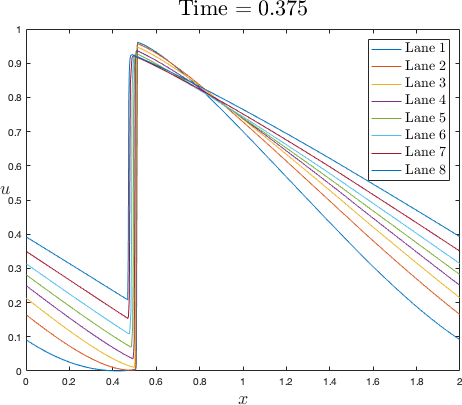 Figure 1
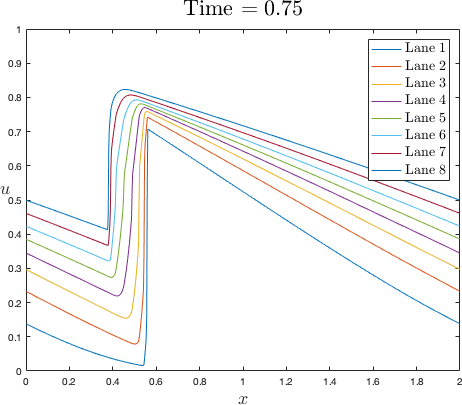 Figure 2
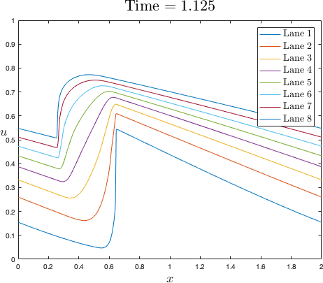 Figure 3
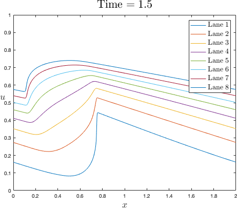 Figure 4
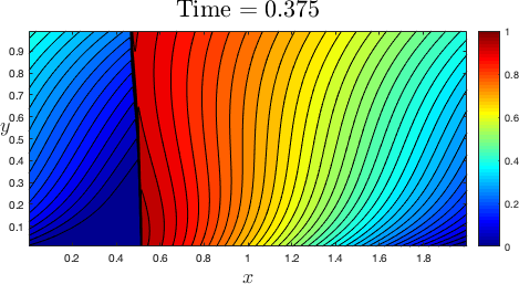 Figure 5
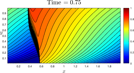 Figure 6
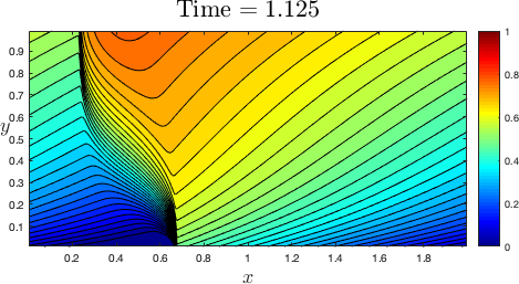 Figure 7
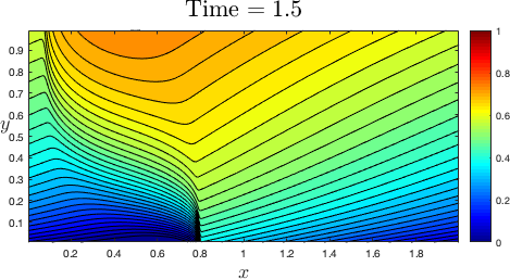 Figure 8
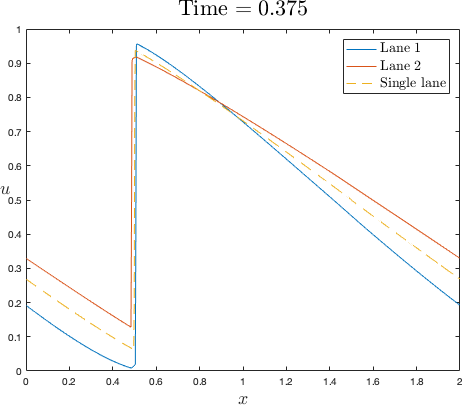 Figure 9
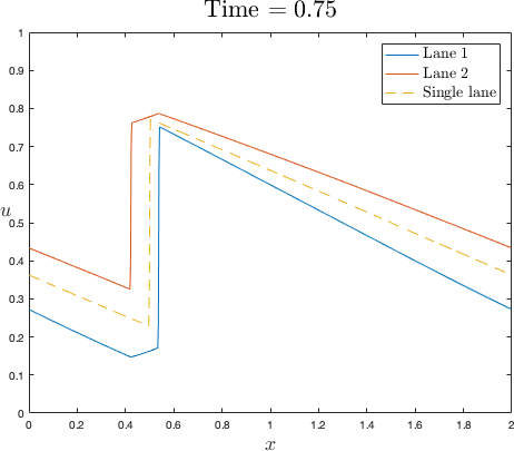 Figure 10
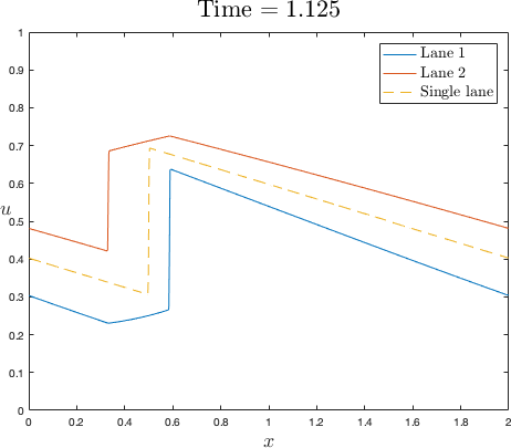 Figure 11
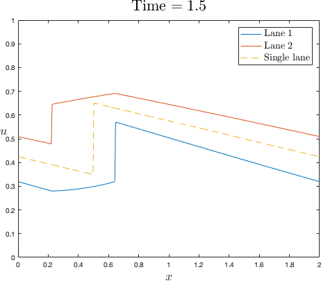 Figure 12
Peer Reviews
No public reviews on file for this paper yet. If you reviewed it on a platform where reviews are public (OpenReview, ICLR, NeurIPS, ICML), you can paste yours below so the community can read it here.
Videos
No videos yet. Explain this paper in a talk, walkthrough, or lecture? Add one.
Models for dense multilane vehicular traffic
Helge Holden
Department of Mathematical Sciences, NTNU Norwegian University of Science and Technology, NO–7491 Trondheim, Norway
[email protected] https://www.ntnu.edu/employees/helge.holden and
Nils Henrik Risebro
Department of Mathematics, University of Oslo, P.O. Box 1053, Blindern, NO–0316 Oslo, Norway
[email protected] https://www.mn.uio.no/math/english/people/aca/nilshr/index.html
Abstract.
We study vehicular traffic on a road with multiple lanes and dense, unidirectional traffic following the traditional Lighthill–Whitham–Richards model where the velocity in each lane depends only on the density in the same lane. The model assumes that the tendency of drivers to change to a neighboring lane is proportional to the difference in velocity between the lanes. The model allows for an arbitrary number of lanes, each with its distinct velocity function.
The resulting model is a well-posed weakly coupled system of hyperbolic conservation laws with a Lipschitz continuous source. We show several relevant bounds for solutions of this model that are not valid for general weakly coupled systems.
Furthermore, by taking an appropriately scaled limit as the number of lanes increases, we derive a model describing a continuum of lanes, and show that the -lane model converges to a weak solution of the continuum model.
Key words and phrases:
Lighthill–Whitham–Richards model, multilane traffic flow, continuum limit.
2010 Mathematics Subject Classification:
Primary: 35L60; Secondary: 35L65, 35L67, 82B21
Research was supported by the grant Waves and Nonlinear Phenomena (WaNP) (no 250070) from the Research Council of Norway.
1. Introduction
The Lighthill–Whitham–Richards (LWR) model for unidirectional traffic on a single road, see [13, 16], reads
[TABLE]
where denotes the density of vehicles at the position and time , and is a given velocity function. The LWR-model expresses conservation of vehicles and is a well-established model for dense unidirectional single lane vehicular traffic on a homogeneous road without exits and entries. Furthermore, it serves as the standard textbook example to gain intuition regarding the behavior of solutions of scalar one-dimensional hyperbolic conservation laws, see, e.g., [10].
Given the importance of vehicular traffic modeling in modern society, it is no wonder that the LWR-model has been generalized to describe several important scenarios in dense traffic flow. Indeed, “traffic hydrodynamics” has become a research field in its own right, where the flow of vehicles is modeled by conservation laws or balance equations. In the general context, the LWR-model is the simplest model among the many hydrodynamic traffic models. Among the other models often used is the Aw–Rascle model [1], which is a system of conservation laws where the velocity is not a given function of , but satisfies a second conservation law. It is thus considerably more complicated than the simple LWR-model. For a general introduction to how conservation laws are used in traffic modeling, see [9, 3] and the many references therein.
In this paper we introduce a new model for multilane dense vehicular traffic where the underlying model for each lane remains the LWR-model. Our basic assumption is that drivers prefer to drive faster, and that the tendency of a vehicle to change lane is proportional to the difference in velocity between neighboring lanes. If (1.1) describes the density of vehicles in a particular lane, the multilane behavior is described by a source term, accounting for lane changes. The result is thus a system of weakly coupled scalar conservation laws.
More precisely, consider two lanes denoted and , the model we study, reads
[TABLE]
where the change of lanes is codified in
[TABLE]
Here denotes the density in lane . The system constitutes a weakly coupled system of one-dimensional hyperbolic conservation laws, and there is ample theory available for systems of this type, see Section 2. The system readily generalizes to an arbitrary number of lanes, see Section 3. We show that the general system with lanes has a unique entropy solution, and that the solution is well-posed in the sense that one has a surprising stability
[TABLE]
for two solutions and , see Theorems 3.2 and 3.3. Note that the stability does not hold in general for systems of balance laws, that is, hyperbolic conservation laws with source.
The models invites for considering the continuum limit where the number of lanes increases to infinity. We organize the parallel lanes along the -axis, and measure the distance between the lanes along the -axis. The distance between the lanes is scaled as , where denotes the number of lanes. For simplicity we assume that the velocity function is given by where , and is the velocity function. We scale the function such that and . We need to scale the constant as . We consider given initial data , where the initial data for lane is is given by (4.20) and with solution . We interpolate this function to where . We assume that is smooth and positive with . In Theorem 4.2 we show that where is a weak solution of
[TABLE]
where the flux function is defined as . This equation is an interesting anisotropic and degenerate parabolic equation with non-trivial boundary conditions in the -direction.
There is a plethora of approaches to the modeling of multilane dense traffic, and the most relevant to our approach here can be found in [5, 11, 12, 14], using either kinetic models or the Aw–Rascle model or variations thereof, or [2, 4] where more involved source terms modeling the change of lanes, are employed. See [15] for a survey of various models for lane changing.
The rest of this paper is organized as follows: In Section 2 we detail the two-lane case, and show that is an invariant region. In Section 3 we state the -lane model, and prove a number of estimates on the solution. Finally, in Section 4, we study the limit as . See [6] for a model for two-dimensional traffic flow on highways. Analogously to the analysis of numerical schemes for degenerate parabolic equations, we establish enough estimates on the solution, enabling us to conclude that a limit exists, and that this limit is a weak solution of a degenerate convection-diffusion equation. All sections are illustrated by numerical examples.
2. A continuum model for two-lane vehicular traffic
Consider a road with two lanes, each with its own velocity function. The lanes are homogeneous, and traffic on the road is unidirectional. We assume that the vehicular traffic is dense, allowing for a continuum formulation. Let and denote the density and velocity, respectively, in lane .
In this paper we focus on the interaction between the two lanes. We assume that drivers prefer to drive in the faster lane, and the tendency of a vehicle to change lane is proportional to the difference in velocity. Thus the flow from lane to lane equals
[TABLE]
where is a constant, and . The flow from lane to lane equals . The classical Lighthill–Whitham–Richards model implies the following model describing the two-lane traffic
[TABLE]
where is the position along the road and denotes time. This system of hyperbolic conservation laws is weakly coupled with a Lipschitz continuous source term.
The velocities are strictly decreasing positive functions, and we assume that they are scaled such that . For simplicity, we scale space and time such that .
It is well-known that this system in general only allows for weak solutions , the set of integrable functions of finite total variation, see, e.g., [10]. Furthermore, the issue of uniqueness of the solution is non-trivial and one needs to require that the solution satisfies an entropy condition.
Definition 2.1**.**
Let be strictly decreasing positive functions such that . Assume that for . We say that with for is a weak solution of (2.2) with initial data if
[TABLE]
for all compactly supported test functions .
The solution is called an entropy solution if
[TABLE]
for all convex functions where satisfies with , and for all compactly supported non-negative test functions , .
Remark 2.2**.**
It suffices that (2.3) holds for of the form for all constants , see [10, Remark 2.1]. In that case .
Remark 2.3**.**
The existence and uniqueness of entropy solutions to (2.2) follows by Theorem 3.2 below.
We will throughout the paper use the following notation:
[TABLE]
where is the indicator (characteristic) function of a set . Note that
[TABLE]
We shall also employ the convention that denotes a “generic” finite positive constant, independent of critical parameters, whose actual value may change from one occurrence to the next. Similarly, we use to denote a positive function for .
This model (2.2) has the natural invariant region . This is the content of the following lemma.
Lemma 2.4**.**
Let and be entropy solutions in the sense of Definition 2.1, with initial data for . If for all and , then for all and for .
Proof.
To show that if we use the entropy . Then
[TABLE]
in for . We use a non-negative test function to find that
[TABLE]
Adding these two equations and using that , we get
[TABLE]
with
[TABLE]
We have that
[TABLE]
Hence for almost all .
Similarly, by using the convex entropy we get
[TABLE]
in , the set of distributions. By the same argument as before, we arrive at
[TABLE]
with
[TABLE]
We have that
[TABLE]
if and are non-negative. ∎
Remark 2.5**.**
There are also other invariant regions for this equation. If
[TABLE]
then
[TABLE]
for .
2.1. An example
We finish our discussion of the two-lane case by exhibiting an example. The velocities on the two roads are
[TABLE]
and the initial data
[TABLE]
Of course, we do not have entropy solutions in closed form, so instead we use a numerical approximation generated by the Engquist–Osher scheme with grid points in the interval . Figure 1 shows the computed solution at , , and . For comparison, we have also included the single lane model with the (average of and ) speed . We see that there is the expected change of lane to the faster lane, and that a shock builds up in the fast lane to the left of the shock in the slow lane.
3. Multilane model
The model (2.2) can be generalized to an arbitrary number of lanes. Consider a road with lanes. Traffic is unidirectional and dense. Each lane has its specific velocity function depending only on the density in that lane, thus , where is the density in lane .
Assume that drivers prefer to drive in the faster lane, and this tendency increases with the velocity difference with adjacent lanes. Thus the flow from lane to lane equals
[TABLE]
where we have scaled time such that the constant of proportionality is one. We then get, in the analogous manner to the derivation of (2.2), that
[TABLE]
coupled with the boundary conditions
[TABLE]
Definition 3.1**.**
Let be Lipschitz continuous functions, and assume that , for . We say that is a weak solution of (3.1) with initial data if
[TABLE]
for all compactly supported test functions .
It is an entropy solution if
[TABLE]
for all convex functions , and for all non-negative test functions . Here is defined by with .
The wellposedness of the system of equations (3.1) is ensured by the following general theorem from [8], see also [7].
Theorem 3.2** ([7], Theorem 3.13).**
Assume that and are as in Definition 3.1. The there exists a unique entropy solution . Furthermore, if is another entropy solution with initial data , then
[TABLE]
A fundamental property of hyperbolic conservation law is the contractivity of solutions in the sense that the spatial -norm of the difference between two entropy solutions at a specific time does not increase in time. This property is in general lost for weakly coupled systems, or for scalar conservation laws with a source. The general bound (3.4) does not imply contractivity. However, for the system (3.1), the special form of the source yields contractivity for the whole solution, as the next theorem shows.
Theorem 3.3**.**
Consider two entropy solutions and of (3.1) with initial data and , respectively. Then we have
[TABLE]
Proof.
By using Kružkov’s doubling of variables technique we get
[TABLE]
in . Subtracting the equation for and adding the equation for we arrive at
[TABLE]
in . Choosing we infer that
[TABLE]
Recall that
[TABLE]
Now
[TABLE]
So if ,
[TABLE]
where . Therefore
[TABLE]
Define
[TABLE]
then (3.6) and the above inequality imply that
[TABLE]
Gronwall’s inequality then implies that
[TABLE]
Thus if , i.e., , then for , i.e., .
By the Crandall–Tartar lemma [10, Lemma 2.13], this implies contractivity, i.e., if and are entropy solutions to (3.1) with initial data and , then (3.5) holds for . ∎
One way to enforce the boundary conditions (3.2), is to define , , and . Henceforth we will use this convention.
Corollary 3.4**.**
Consider two solutions and of (3.1) with initial data and , respectively, in the sense of Definition 3.1. Then we have
[TABLE]
Furthermore, we have
[TABLE]
In addition
[TABLE]
Proof.
Setting for yields (3.7). Similarly, defining , using (3.5), and sending to zero gives (3.8). To obtain time continuity we define , to get (3.9). ∎
We also note the following useful estimates. Define and , divide by and let to find that
[TABLE]
If we assume that the quantity on the left is bounded by , then we get
[TABLE]
Furthermore, we have the useful observation
[TABLE]
3.1. An example
We also here include an example. For we set , and define
[TABLE]
Also in this case the depicted solutions were calculated with the Engquist–Osher scheme with grid points in the interval . Figure 2 shows the computed solutions at , , and . We see the expected change of lanes to the faster lanes, and that a shock builds up in the faster lanes to the left of the slower lanes.
4. Infinitely many lanes — the continuum limit
It is natural, at least mathematically, to consider the case where the lanes increase in number while at the same time get closer. Our aim in this section is therefore to investigate limit as in the system in the previous section.
To this end we let (the number of lanes) be a positive integer and set . Let for . We shall also use the “divided difference” notation
[TABLE]
For simplicity, we restrict our presentation to the case where where is a differentiable function with , and . Define . Throughout we will use the notation , and . Now we reintroduce the scaling constant in (2.1), and set . For the convenience of the reader we set . Thus, for , is the unique entropy (in the sense of Definition 3.1) solution of the balance equation
[TABLE]
with the boundary conditions
[TABLE]
It is also useful to define the function by
[TABLE]
We shall investigate whether the family , is compact and characterize the limit . To this end we must show a number of estimates.
The right-hand side of (4.1) equals
[TABLE]
Thus (4.1) reads
[TABLE]
for , and we have the boundary values
[TABLE]
Remark**.**
Observe that the above term is an upwind discretization of the transport term corresponding to , with .
Similarly to (4.3), we also get the expression
[TABLE]
Recall (3.3) with and an approximation to . That gives
[TABLE]
where . We can sum this for , multiply with and do a summation by parts to get
[TABLE]
It will be useful to lower bound the last two terms on the left-hand side.
Recall first that
[TABLE]
for some constant independent of . Using this and the fact that is bounded, as well as
[TABLE]
we have that
[TABLE]
Furthermore, note that the same argument yields
[TABLE]
Observe that
[TABLE]
and then use the inequality . Thus, since ,
[TABLE]
where . Similarly,
[TABLE]
and therefore
[TABLE]
Note that due to the monotonicity of we have for some between and ,
[TABLE]
We can now estimate the last two terms of the left-hand side of (4.7) from below. More precisely,
[TABLE]
which we can rewrite as
[TABLE]
This implies that
[TABLE]
and
[TABLE]
Observe that by (4.9), (4.12) follows from (4.13), viz.
[TABLE]
By the same procedure, starting with (4.4) but using the alternate form (4.6) of the right-hand side, we arrive at the bounds
[TABLE]
and
[TABLE]
Combining the two bounds (4.12) and (4.14) we get
[TABLE]
In a similar manner, we find
[TABLE]
The other two bounds, (4.13) and (4.15) can be used for a continuity estimate. Write and compute for
[TABLE]
Squaring and integrating over gives
[TABLE]
By direct computations we have that
[TABLE]
which gives
[TABLE]
Multiplying with summing over and integrating in , , gives the bound, using (4.18) with , and (4.17),
[TABLE]
Note that this also follows from (4.13), using that .
Convergence
We assume that is such that and that . Now we assume that the initial data are such that there is a function such that
[TABLE]
where and . Furthermore . Since ,
[TABLE]
for some constant which is independent of . For convenience, we have set and .
We assume that is given, such that , and for . Define . Let be the entropy solutions to (4.4) with the boundary conditions
[TABLE]
which actually is a special case of (4.5). Then we define
[TABLE]
for and if . We have that , , and, using the bounds (3.7) and (3.8), , where is independent of . Furthermore, using (4.18),
[TABLE]
where is independent of . This is sufficient to conclude that there is a function and a sequence , as , such that
[TABLE]
Furthermore, we have that , therefore . The bound (4.19) ensures that .
Definition 4.1**.**
Set and . Let be as above, in particular . We say that , such that , is a weak solution to
[TABLE]
if for all test functions ,
[TABLE]
The aim is now to show that the limit is a weak solution in the above sense. Since is a weak solution of (4.4), we have
[TABLE]
for . We use where
[TABLE]
for a suitable test function . Next we multiply with and sum over and do a summation by parts on the terms which have . This will give us the weak formulation for . For simplicity we assume that , so that the whole sequence converges. Term by term we get
[TABLE]
as .
Turning to (4.22), we have that
[TABLE]
where is between and and is between and . Therefore
[TABLE]
The last term here vanishes as since
[TABLE]
where we used (4.13). Hence
[TABLE]
as .
Now for (4.23), we have
[TABLE]
using (4.8), (4.16), and interpolation between and . Thus \Delta y\bigl{|}\sum_{i=1}^{N}\text{\eqref{eq:term3}}\bigr{|}\rightarrow 0 as .
It is straightforward to show that
[TABLE]
Hence, the limit is a weak solution.
We can sum up the result of our arguments in the following theorem.
Theorem 4.2**.**
Let such that , and for all , and assume that is a strictly increasing differentiable function such that and .
Assume that and let be defined in (4.2) where solves (4.1) for .
Then there exists a sequence and correspondingly such that the sequence of solutions has a limit, i.e.,
[TABLE]
The limit is a weak solution according to Definition 4.1.
We also have the regularity estimate
[TABLE]
4.1. An example
To illustrate the continuum limit, we have tested the “same” initial value problem as in Section 2.1 and Section 3.1. The relevant data are
[TABLE]
and
[TABLE]
We have used (i.e., 60 lanes) and solved (4.1) using the Engquist–Osher scheme with grid points in the interval . Figure 3 shows the computed density at four different times. It is illuminating to compare this figure with Figures 1 and 2.
The reference list from the paper itself. Each links out to its DOI / PubMed record.
- 1[1] A. Aw and M. Rascle. Resurrection of “second order” models of traffic flow. SIAM J. Appl. Math. , 60(3):916–938, 2000.
- 2[2] R.M. Colombo and A. Corli. Well posedness for multilane traffic models. Ann. Univ. Ferrara Sez. VII Sci. Mat. , 52(2):291–301, 2006.
- 3[3] M. Garavello, Ke Han, and B. Piccoli. Models for Vehicular Traffic on Networks , volume 9 of AIMS Series on Applied Mathematics . American Institute of Mathematical Sciences (AIMS), Springfield, MO, 2016.
- 4[4] J.M. Greenberg, A. Klar, and M. Rascle. Congestion on multilane highways. SIAM J. Appl. Math. , 63(3):818–833, 2003.
- 5[5] D. Helbing and A. Greiner. Modeling and simulation of multilane traffic flow. Phys. Rev. E , 55(5):5498–5508, 1997.
- 6[6] M. Herty, A. Fazekas, and G. Visconti. A two-dimensional data-driven model for traffic flow on highways. Netw. Heterog. Media , 13(2):217–240, 2018.
- 7[7] H. Holden, K.H. Karlsen, K.-A.Lie, and N.H. Risebro. Splitting Methods for Partial Differential Equations with Rough Solutions. Analysis and MATLAB programs. EMS Series of Lectures in Mathematics. European Mathematical Society (EMS), Zürich, 2010.
- 8[8] H. Holden, K.H. Karlsen, and N.H. Risebro. On uniqueness and existence of entropy solutions of weakly coupled systems of nonlinear degenerate parabolic equations. Electron. J. Differential Equations , pages No. 46, 31, 2003.