Nonlinear Stochastic Position and Attitude Filter on the Special Euclidean Group 3
Hashim A. Hashim, Lyndon J. Brown, Kenneth McIsaac

TL;DR
This paper develops a nonlinear stochastic filter directly on SE(3) for pose estimation, ensuring bounded errors and convergence despite high noise, demonstrated through simulations showing robustness and effectiveness.
Contribution
It introduces a novel stochastic pose filter on SE(3) with proven stability and convergence properties, handling high noise and bias in measurements.
Findings
Errors are semi-globally uniformly ultimately bounded in mean square.
Errors converge to a small neighborhood of the origin in probability.
Simulation results confirm robustness against high noise and bias.
Abstract
This paper formulates the pose estimation problem as nonlinear stochastic filter kinematics evolved directly on the Special Euclidean Group SE(3). Proposed filter guarantees that the errors present in position and Rodriguez vector estimates are semi-globally uniformly ultimately bounded (SGUUB) in mean square, and that they converge to small neighborhood of the origin in probability. Simulation results show the robustness and effectiveness of the proposed filter in presence of high levels of noise and bias associated with the velocity vector as well as body-frame measurements. Keywords: Pose estimator, pose observer, attitude estimate, control, estimator, observer, Nonlinear stochastic pose filter, stochastic differential equations, Brownian motion process, Ito, Stratonovich, Wong Zakai, unit-quaternion, special orthogonal group, homogeneous transformation matrix, complimentary filter,…
Click any figure to enlarge with its caption.
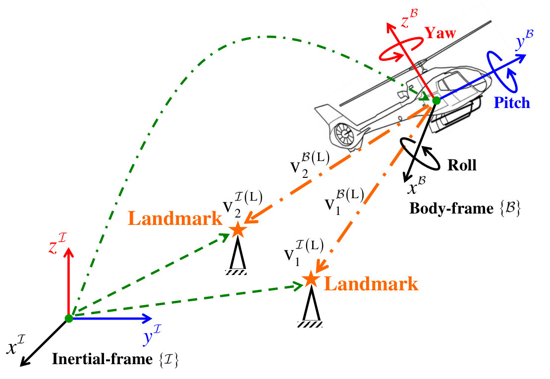 Figure 1
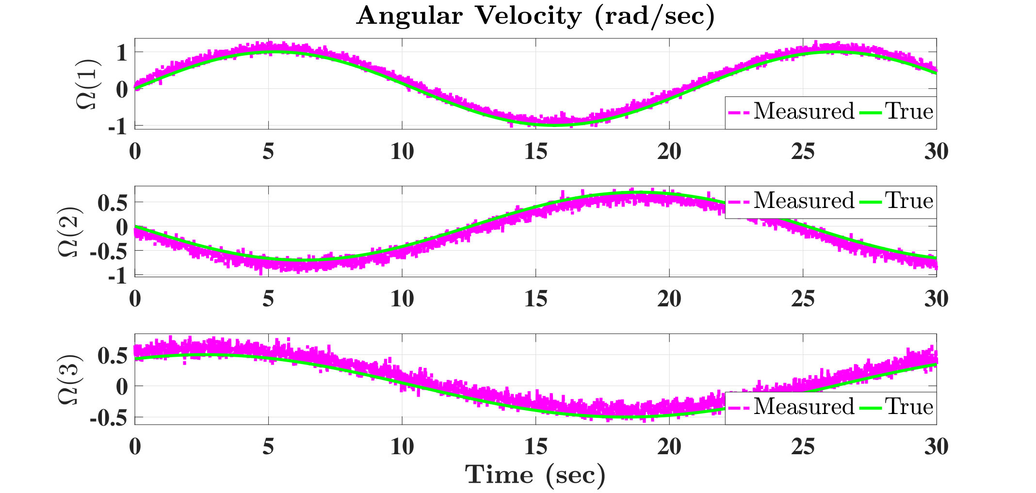 Figure 2
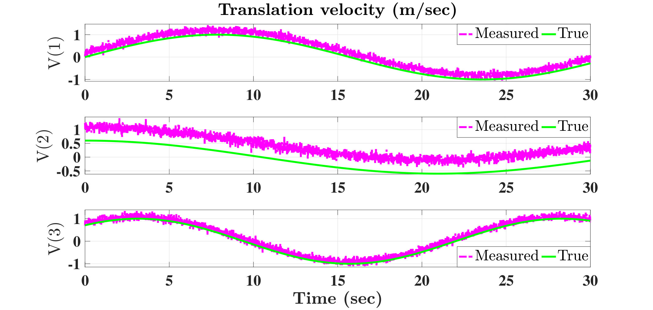 Figure 3
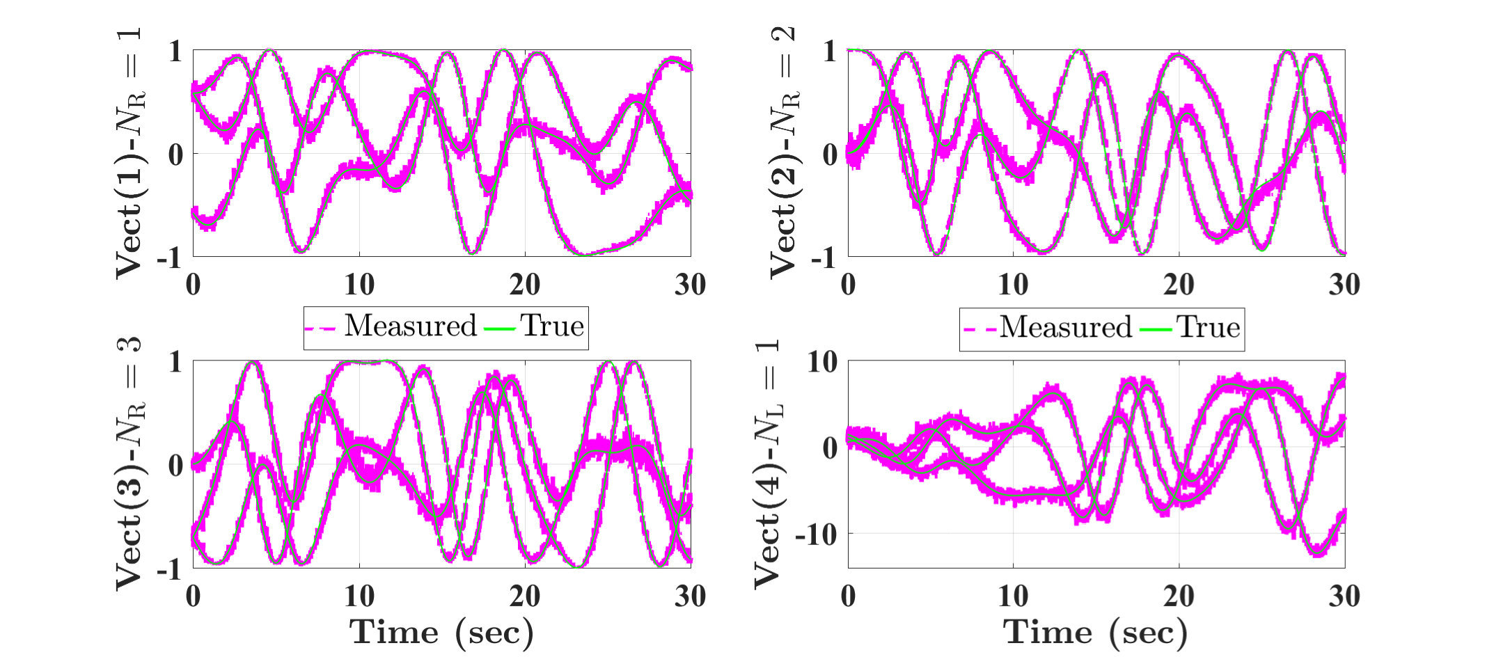 Figure 4
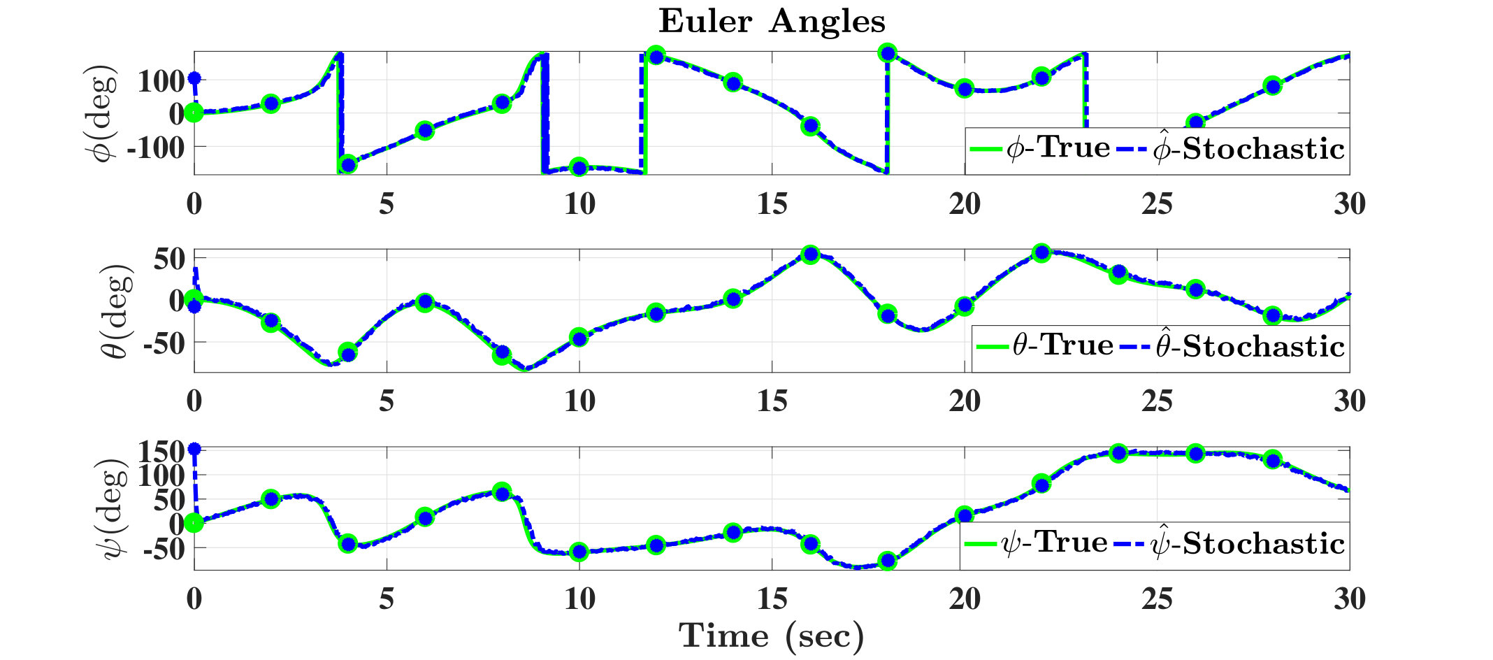 Figure 5
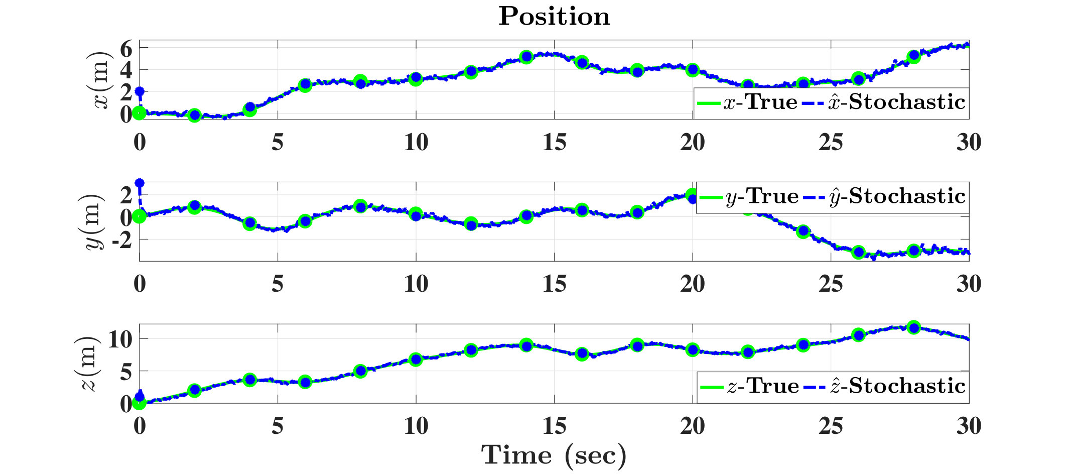 Figure 6
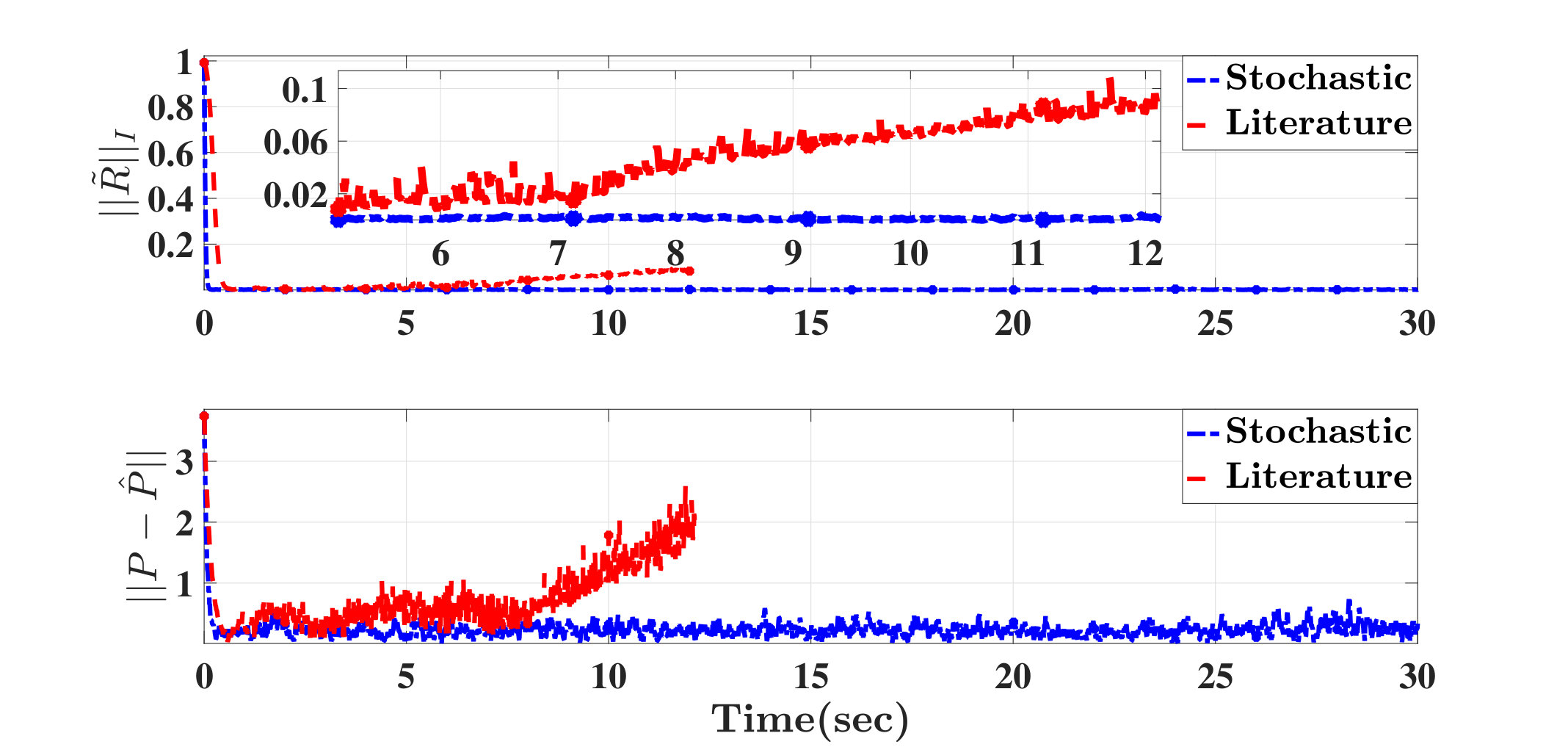 Figure 7
| Input measurements | |||||
|---|---|---|---|---|---|
| Index | |||||
| Mean | |||||
| STD | |||||
| Output data over the period (1-30 sec) | |||||
| Index | |||||
| Mean | |||||
| STD | |||||
Peer Reviews
No public reviews on file for this paper yet. If you reviewed it on a platform where reviews are public (OpenReview, ICLR, NeurIPS, ICML), you can paste yours below so the community can read it here.
Videos
No videos yet. Explain this paper in a talk, walkthrough, or lecture? Add one.
Nonlinear Stochastic Position and Attitude Filter on the Special Euclidean Group 311footnotemark: 1
Hashim A. Hashim
Lyndon J. Brown
Kenneth McIsaac
Department of Electrical and Computer Engineering, University of Western Ontario, London, ON, N6A-5B9, Canada
Abstract
This paper formulates the pose (attitude and position) estimation problem as nonlinear stochastic filter kinematics evolved directly on the Special Euclidean Group . This work proposes an alternate way of potential function selection and handles the problem as a stochastic filtering problem. The problem is mapped from to vector form, using the Rodriguez vector and the position vector, and then followed by the definition of the pose problem in the sense of Stratonovich. The proposed filter guarantees that the errors present in position and Rodriguez vector estimates are semi-globally uniformly ultimately bounded (SGUUB) in mean square, and that they converge to small neighborhood of the origin in probability. Simulation results show the robustness and effectiveness of the proposed filter in presence of high levels of noise and bias associated with the velocity vector as well as body-frame measurements.
keywords:
Pose estimator, position, attitude, nonlinear stochastic filter, stochastic differential equations, Brownian motion process, Ito, Stratonovich, Wong-Zakai, Rodriguez vector, special Euclidean group, special orthogonal group, SE(3), SO(3).
To cite this article: \textcolor**redH. A. Hashim, L. J. Brown, and K. McIsaac, ”Nonlinear Stochastic Position and Attitude Filter on the Special Euclidean Group 3,” Journal of the Franklin Institute, vol. 356, no. 7, pp. 4144-4173, 2019.
**
**The published version (DOI) can be found at: 10.1016/j.jfranklin.2018.12.025
**
Please note that where the full-text provided is the preprint version** and this may differ from the revised and/or the final Published
**
version. To cite this publication, please use the final published version.
Personal use of this material is permitted. Permission from the author(s) and/or copyright holder(s), must be obtained for all other uses, in any current or future media, including reprinting or republishing this material for advertising or promotional purposes.
**Please contact us and provide details if you believe this document breaches copyrights. We will remove access to the work immediately and investigate your claim. **
1 Introduction
This paper concerns the problem of position and attitude estimation of a rigid-body moving in 3D space which is commonly known as the pose problem. Pose (attitude and position) estimation is a crucial task in robotics and engineering applications. The attitude and position can be reconstructed through a set of vector measurements with respect to body and inertial frames of reference. In general, the main objective of pose estimation problem is to minimize the cost function similar to Wahba’s problem [1]. The approach applied in [1] was purely algebraic, whereas other algorithms used singular value decomposition to obtain comparable static solution [2]. However, the set of vectorial measurements is susceptible to uncertainties such as slowly time-variant bias and random noise components. Therefore, the static solutions proposed in [1, 2] give poor results. Traditionally, the attitude estimation problem has been handled using Gaussian filters or nonlinear deterministic filters which aimed to converge any initialized estimate to the solution [3, 4, 5]. The family of Gaussian attitude filters includes Kalman filter (KF) [6], extended KF (EKF) [7, 8], multiplicative EKF (MEKF) [9], and invariant EKF (IEKF) [10]. A good survey of Gaussian attitude filters can be found in [4]. Gaussian attitude filters often consider the unit quaternion in attitude representation and go through liberalizations. From the other side, the attitude problem is naturally nonlinear and nonlinear deterministic attitude filters can be developed directly on the Special Orthogonal Group as a deterministic problem (for example [11, 12, 13]). In fact, nonlinear deterministic attitude filters are simpler in derivation and representation. In addition, they require less computational power and demonstrate better tracking performance in comparison with Gaussian filters [4, 11, 3]. Therefore, it is better to address the attitude and attitude-position filtering in a nonlinear sense.
Inertial measurement units (IMUs) have a prominent role in enriching the research of attitude estimation. These units are inexpensive fostering the researchers to propose nonlinear deterministic filters on [11, 12, 13]. Attitude estimation is an essential part of the pose estimation problem and a critical task in the estimation process. Accordingly, the pose estimation problem can be modeled and solved using a nonlinear deterministic filter evolved on the Special Euclidean Group . Recently, the design of pose filters received considerable attention [14, 15, 16, 17, 18, 19]. A computer vision system that employs a monocular camera with IMUs was developed for pose estimation [14, 15]. The filter in [15] evolved directly on and has been proven to be exponentially stable. However, the filter requires attitude and position reconstruction for implementation. Later, the nonlinear complementary filter that evolved directly on in [15] was modified using vectorial measurements without the need of attitude and position reconstruction [16, 17]. For a good overview of pose estimation on the reader is advised to visit [20]. Despite the simplicity of the filter design in [15, 16, 17], simulation results showed high sensitivity to noise and bias introduced in the measurements. Moreover, pose estimators such as [14, 15, 16, 17, 18] disregard the noise in the filter design assuming only constant bias introduced in the measuring process. Therefore, successful spacecraft control applications, such as, [21, 22, 23] cannot be achieved without pose filters robust against uncertain measurements.
Therefore, in order to develop successful pose estimator, we need to realize that
the pose problem is naturally nonlinear on ; and 2. 2)
the true pose kinematics rely on angular and translational velocity.
However, the velocity vector is subject to slowly time-variant bias and random noise components. Hence, in this work a nonlinear stochastic position and attitude filter is developed on in the sense of Stratonovich [24]. The problem is mapped from to vector form which includes position and Rodriquez vector such that . In the case where the velocity measurements are corrupted with noise, the aim is
to steer the error vectors towards an arbitrarily small neighborhood of the origin in probability; 2. 2)
to attenuate the noise impact for known or unknown bounded covariance; and 3. 3)
to show that the error in and estimates is semi-globally uniformly ultimately bounded (SGUUB) in mean square.
The rest of the paper is organized as follows: Section 2 presents an overview of mathematical notation, mapping from to angle-axis and Rodriguez vector parameterization, properties and some helpful properties for the nonlinear stochastic position and attitude filter design on . Pose estimation dynamic problem in the stochastic sense is presented in Section 3. The nonlinear stochastic filter on and the stability analysis are presented in Section 4. Section 5 demonstrates numerical results and shows the output performance of the proposed stochastic filter. Finally, Section 6 draws a conclusion of this work.
2 Mathematical Notation and Background
Throughout this paper, denotes the set of nonnegative real numbers. is the real -dimensional space, denotes the real dimensional space. For , the Euclidean norm is defined by where ⊤ is the transpose of the associated component. denotes the set of functions with continuous th partial derivatives. denotes a set of continuous and strictly increasing functions such that and vanishes only at zero. denotes a set of continuous and strictly increasing functions which belong to class and is unbounded. is a probability and is an expected value of the associated component. is the set of singular values of associated matrix with being the minimum value. Also, denotes identity matrix with -by- dimensions, is a zero vector with rows and one column, and . is a potential function, and for we have and .
Notation for frames is as follows: denotes the body-frame and denotes the inertial-frame. Let denote the 3 dimensional general linear group. is a Lie group characterized by smooth multiplication and inversion. The set of orthogonal group, is a subgroup of the general linear group and is defined by
[TABLE]
where is the identity matrix. denotes the Special Orthogonal Group and is a subgroup of the orthogonal group and the general linear group. The attitude of a rigid body is denoted by a rotational matrix , and is defined as follows
[TABLE]
where is the determinant of the associated matrix. Let denote the Special Euclidean Group with . is a subset of the affine group such that
[TABLE]
where is known as the homogeneous representation or the transformation matrix of the rigid body and is defined by
[TABLE]
with denoting position, denoting the attitude of the rigid-body in the space, and being a zero row. The associated Lie-algebra of is termed and is defined by
[TABLE]
with being the space of skew-symmetric matrices. Let us define the map such that
[TABLE]
For all , we have where is the cross product between the two vectors. Let be the wedge operator, and the wedge map such that
[TABLE]
where for . The Lie algebra of is denoted by and given by
[TABLE]
Let the operator be the inverse of , denoted by such that for and we have
[TABLE]
Let denote the anti-symmetric projection operator on the Lie-algebra , defined by such that
[TABLE]
Let us define as the composition mapping such that . Hence, can be expressed for as
[TABLE]
Consider denoting the projection operator on the space of the Lie algebra such that for \mathcal{M}=\left[\begin{array}[]{cc}M&m_{x}\\ m_{y}^{\top}&m_{z}\end{array}\right]\in\mathbb{R}^{4\times 4} with , and , we have
[TABLE]
For any , we define the operator as follows
[TABLE]
The normalized Euclidean distance of a rotation matrix on is defined by
[TABLE]
such that is the trace of the associated matrix, while the normalized Euclidean distance of is . The orientation of a rigid-body rotating in a 3D space can be established according to its angle of rotation and its axis parameterization [25]. Such parameterization is termed angle-axis parameterization. Mapping from angle-axis parameterization to is given by such that
[TABLE]
In the same spirit, the orientation of a rigid-body can be constructed by Rodriguez parameters vector. Mapping from Rodriguez vector parameterization to is defined by such that
[TABLE]
One can obtain the normalized Euclidean distance in (6) as a function of Rodriguez parameters vector substituting (8) into (6) to yield
[TABLE]
Also, the anti-symmetric projection operator of the attitude , denoted by , can be defined in terms of Rodriguez parameters vector from (8) as
[TABLE]
Accordingly, the composition mapping of in (2) and (3) can be defined in terms of Rodriguez parameters vector as
[TABLE]
[TABLE]
Let us consider the transformation matrix in (1) with . The adjoint map for any and is given by
[TABLE]
Let us define another adjoint map for any by
[TABLE]
One can easily verify that the vex operator in (5) can be combined with the results in (12) and (13) to show
[TABLE]
thus
[TABLE]
which will be useful for the filter derivation and further analysis. Finally, the following identities will be used in the subsequent derivations
[TABLE]
3 Problem Formulation in Stochastic Sense
The orientation of a rigid-body rotating in 3D space is normally defined in terms of the body-frame relative to the inertial-frame . Let be the position of the rigid-body measured on the inertial-frame . Thereby, this work concerns position as well as attitude estimation of a rigid-body moving and rotating in 3D space. Consider the homogeneous transformation matrix given by
[TABLE]
Let and be angular and translational velocity of a moving rigid-body attached to the body-frame, respectively, for all . Hence, the dynamics of the homogeneous transformation matrix are expressed by
[TABLE]
where is the group velocity vector expressed relative to the body-frame. The homogeneous transformation matrix can be reconstructed through a set of known vectors in the inertial-frame and their measurements in the body-frame. Let the superscript and denote the associated body-frame and inertial-frame of the component, respectively. The pose estimation problem is illustrated in Figure 1.
Assume that there exists a number of feature points or landmarks denoted by such that
[TABLE]
with being the landmark measurement in the body-frame and being a known constant feature in the inertial-frame for all . Also, and are unknown bias and noise vectors attached to the th measurement for all . The position can be simply constructed if the attitude matrix is available. Let us denote the set of vectors associated with landmarks by
[TABLE]
A weighted geometric center is considered for the case of more than one landmark is available for measurement. The center is given by
[TABLE]
with refers to the confidence level of the th measurement. On the other side, the attitude matrix can be obtained through a set of -known non-collinear vectors. The vectors are measured in the moving frame . Let be a measured vector in the body-frame such that the th body-frame vector is given by
[TABLE]
where refers to the known vector in the inertial-frame for . and represent the unknown bias and noise components attached to the th measurement, respectively, for all . Let us denote the set of vectors associated with attitude reconstruction by
[TABLE]
Assumption 1
At least one feature point is available for measurements (22) with , and three non-collinear vectors are available for measurements (26) with . In case when , the third vector can be obtained by and .
According to Assumption 1, means that the set of vectorial measurements in (27) is sufficient to have rank 3. The homogeneous transformation matrix can be reconstructed if Assumption 1 is satisfied. It is common to obtain the normalized values of inertial and body-frame measurements in (26) such that
[TABLE]
and the normalized set of (28) is
[TABLE]
In that case, the attitude can be extracted knowing and instead of and . Gyroscope obtains the measurements of angular velocity in the body-frame and the measurement vector is defined by
[TABLE]
with denoting the true value of angular velocity, denoting the bias component which is unknown constant or slowly time-varying vector, and being the unknown noise component attached to angular velocity measurements. Also, the translational velocity is expressed in the body-frame and its measurement is defined by
[TABLE]
where denotes the true value of the translational velocity, denotes the unknown bias component, and is the unknown noise component attached to translational velocity measurements. Let the group of velocity measurements, bias and noise vectors be defined by , and , respectively, for all . The noise vector is assumed to be Gaussian with zero mean. The dynamics of (20) can be mapped to Rodriguez vector and expressed as follows [25]
[TABLE]
Therefore, the dynamics of the homogeneous transformation matrix in (21) can be mapped to vector form in the sense of Rodriguez parameters from (32) and (8) as
[TABLE]
where as given in (8). According to (30) and (31), the measurements of angular and translational velocities are subject to noise and bias components. These components are characterized by randomness and uncertainty. As such, random behavior and the randomness in measurements could lead to unknown behavior [3, 26, 27] and impair the whole estimation process. The dynamics of the homogeneous transformation matrix in (21) become
[TABLE]
In view of (21) and (33), the dynamics in (34) can be mapped in the same sense and represented as
[TABLE]
where is a continuous Gaussian random noise vector with zero mean which is bounded. The derivative of any Gaussian process yields a Gaussian process [28, 29]. Hence, the vector can be written as a function of Brownian motion process vector with such that
[TABLE]
where and is a diagonal matrix whose diagonal has unknown time-variant nonnegative components defined by
[TABLE]
where is associated with and is associated with . In addition, is a covariance component associated with the noise vector . The properties of Brownian motion process are defined by [29, 30, 31]
[TABLE]
Let the dynamics of the homogeneous transformation in (21) be defined in the sense of Stratonovich [24] and substitute by . Accordingly, the stochastic differential equation of (21) can be expressed as
[TABLE]
in view of (34) and (35), the stochastic differential equation in (36) is given by
[TABLE]
Let us define
[TABLE]
with , and . is locally Lipschitz in and is locally Lipschitz in and . Consequently, the dynamic system in (41) has a solution on in the mean square sense and for any and such that , is independent of (Theorem 4.5 [29]). The aim is to achieve adaptive stabilization of an unknown constant bias and unknown time-variant covariance matrix. Let with being the upper bound of such that
[TABLE]
where is the maximum value of the associated covariance element.
Assumption 2
Both and belong to a given compact set and are upper bounded by a scalar such that .
Definition 1
[32]** The trajectory of the stochastic differential system in (41) is said to be semi-globally uniformly ultimately bounded (SGUUB) if for some compact set and any , there exists a constant , and a time constant such that .
Definition 2
Consider the stochastic differential system in (41) with . For a given function the differential operator is given by
[TABLE]
such that , and .
Lemma 1
[31, 32, 33]** Consider the dynamic system in (41) with potential function , such that , class function and , constants and and a nonnegative function such that
[TABLE]
[TABLE]
then for , there exists almost a unique strong solution on for the dynamic system in (41). The solution is bounded in probability such that
[TABLE]
Moreover, if the inequality in (51) holds, then in (41) is SGUUB in the mean square. Also, when , , , and is continuous, the equilibrium point is globally asymptotically stable in probability and the solution of satisfies
[TABLE]
The proof of this lemma and the existence of a unique solution can be found in [31]. For a rotation matrix , let us define by . The set is forward invariant and unstable for the dynamic system (20) and (21), as implies [25, 3]. From almost any initial condition such that or equivalently , we have and the trajectory of converges to the neighborhood of the equilibrium point conditioned on the value of in (50).
Lemma 2
(Young’s inequality) Let and be real values such that . Then, for any positive real numbers and satisfying with appropriately small positive constant , the following inequality holds
[TABLE]
4 Nonlinear Stochastic Complementary Filter on
Let be the estimator of the homogeneous transformation matrix such that
[TABLE]
The main purpose of this section is to design a pose estimator to drive . Let us define the error in the estimation of the homogeneous transformation matrix by
[TABLE]
with and . Driving guarantees that and , where is the position error associated with and is the error of Rodriguez vector associated with which is in turn associated with . In this Section, a nonlinear deterministic filter on is presented. This filter is subsequently modified into a nonlinear stochastic filter evolved directly on . The nonlinear stochastic filter is driven in the sense of Stratonovich. For , the error vector is regulated to an arbitrarily small neighborhood of the origin in the case where velocity vector measurements are contaminated with constant bias and random noise at each time instant. Let and denote estimates of unknown parameters , and , respectively. Let the error in vector and be defined by
[TABLE]
4.1 Nonlinear Deterministic Pose Filter
The aim of this subsection is to study the behavior of nonlinear deterministic pose filter evolved directly on in presence of noise in the velocity vector measurements . The attitude can be constructed algebraically given a set of measurements in (27) to form , for example [1, 2]. However, is uncertain and significantly far from the true . The given set of measurements in (29) helps in finding and for a given landmark(s) we have and \boldsymbol{T}_{y}=\left[\begin{array}[]{cc}R_{y}&P_{y}\\ \underline{\mathbf{0}}_{3}^{\top}&1\end{array}\right]. Hence, the filter design aims to use the given measured , and the velocity measurements in (30), and (31) to obtain a good estimate of the true . Consider the nonlinear deterministic pose filter design
[TABLE]
where is a measured vector of angular and translational velocity defined in (30) and (31), respectively, with no noise attached to measurements . is the estimate of the unknown bias vector , , as in (5), , and . Also, \breve{\overline{\mathbf{Ad}}}_{\hat{\boldsymbol{T}}}=\left[\begin{array}[]{cc}\hat{R}&\mathbf{0}_{3\times 3}\\ \left[\hat{P}\right]_{\times}\hat{R}&\hat{R}\end{array}\right], \Gamma=\left[\begin{array}[]{cc}\Gamma_{\Omega}&\mathbf{0}_{3\times 3}\\ \mathbf{0}_{3\times 3}&\Gamma_{V}\end{array}\right]=\gamma\mathbf{I}_{6}, is an adaptation gain with , , and , and are positive constants.
Theorem 1
Consider the homogeneous transformation matrix dynamics in (21) with velocity measurements in (30) and (31). Let Assumption 1 hold and assume that the vector measurements in (26) are normalized to (28). Let be reconstructed using the vector measurement in (22) and (28) , and be coupled with the observer in (61), (64) and (67). In case when velocity vector measurements are subject to constant bias, no noise is introduced to the system , , and , 1) the error vector is uniformly ultimately bounded for all ; and 2) consequently steers to the neighborhood of the equilibrium set .
Proof. Let the error in and be defined as in (59), and (58), respectively. Therefore, the derivative of homogeneous transformation matrix error in (58) can be expressed from (34) and (61) as
[TABLE]
where , and . Considering the math identity in (14), we have . For , and in view of the transformation of (34) into (35), one may write (68) as
[TABLE]
with
[TABLE]
and as given in (8). Consider the following potential function
[TABLE]
for the derivative of (70) is defined by
[TABLE]
substitute for and from (6) and (10), respectively, the result in (76) becomes
[TABLE]
such that , substituting for and from (64) and (67), respectively, with as in (11) yields
[TABLE]
applying Young’s inequality to , one obtains . Define
[TABLE]
therefore, equation (80) becomes
[TABLE]
Let and , thus, the result in (81) implies that and will eventually converge to the compact set
[TABLE]
with
[TABLE]
and
[TABLE]
The result obtained in (81) is similar to Lemma 1.2 in [34] which confirms the result in Theorem 1. Theorem 1 is developed for deterministic observers, assuming absence of noises in the system dynamics. Hence, Lyapunov’s direct method guarantees that for , converges to a small neighborhood of the origin. However, if the velocity vector is contaminated with noise such that , it would no longer be convenient to express the derivative of (70) similar to (76). Therefore, the derivative of (70) should be expressed analogously to the differential operator in Definition 2 and consequently, the covariance matrix appears there. As a result, one solution is to reformulate the potential function in (70) such that and are of order higher than two [31, 33]. Clearly, this is not the case in Theorem 1 as well as in previous studies such as [14, 15, 16, 17, 18].
4.2 Nonlinear Stochastic Pose Filter in Stratonovich Sense
Generally, nonlinear deterministic attitude or attitude-position filters assume that velocity measurements are subject only to constant bias (for example [4, 11, 14, 15, 16, 17]). In contrast, the velocity vector is contaminated not only with bias but also noise components. The added components could impair the estimation process of the true position and attitude. As such, the aim is to design a nonlinear stochastic filter evolved directly on in the sense of Stratonovich [24] considering that measurement in the velocity vector is contaminated with constant bias and a wide-band of Gaussian random noise with zero mean. Stochastic differential equations can be defined and solved in the sense of Ito’s integral [30]. Alternatively, Stratonovich’s integral [24] can be employed for solving stochastic differential equations. The common feature between Stratonovich and Ito integral is that if the associated function multiplied by is continuous and Lipschitz, the mean square limit exists. The Ito integral is defined for functional on which is more natural but it does not obey the chain rule. Conversely, Stratonovich is a well-defined Riemann integral for the sampled function, it has a continuous partial derivative with respect to , it obeys the chain rule, and it is more convenient for colored noise [24, 29]. Hence, the Stratonovich integral is defined for explicit functions of . In case of a wide-band of random colored noise process being attached to the velocity measurements, for with , the solution of (41) is defined by
[TABLE]
if the problem has been considered and solved directly in the sense of Ito, the expected value of (82) is
[TABLE]
Hence, Stratonovich came up with the Wong-Zakai correction factor to balance any colored noise that may be introduced to the system dynamics and to end with . A remarkable advantage of Stratonovich is its applicability to white noise as well as colored noise which makes the filter more robust for real time applications [24, 28, 29]. Let us assume that the attitude dynamics in (41) were defined in the sense of Stratonovich [24]. Therefore, the equivalent Ito [28, 29, 30] can be expressed as
[TABLE]
where both and are defined in (41). is termed the Wong-Zakai correction factor of stochastic differential equations (SDEs) in the sense of Ito [35], and denote th, th and/or th elements of the associated vector or matrix. Assume that . Let , therefore, for
[TABLE]
Thus, one can find that for , can be defined after some steps of calculations as follows
[TABLE]
And , for . This implies that
[TABLE]
Manipulating equations (83), (84) and (85), the stochastic dynamics of the Rodriguez vector can be expressed as
[TABLE]
Assume that the elements of covariance matrix are upper bounded by as given in (48) such that the bound of is unknown for nonnegative elements. Consider the nonlinear stochastic pose filter design
[TABLE]
where denotes the measured vector of angular and translational velocity defined in (30) and (31), respectively. and are estimates of the unknown parameter and , respectively, , as in (5), as given in (10), is the Euclidean distance of as defined in (6), and . Also, \breve{\overline{\mathbf{Ad}}}_{\hat{\boldsymbol{T}}}=\left[\begin{array}[]{cc}\hat{R}&\mathbf{0}_{3\times 3}\\ \left[\hat{P}\right]_{\times}\hat{R}&\hat{R}\end{array}\right], \Gamma=\left[\begin{array}[]{cc}\Gamma_{\Omega}&\mathbf{0}_{3\times 3}\\ \mathbf{0}_{3\times 3}&\Gamma_{V}\end{array}\right]=\gamma\mathbf{I}_{6}, and \Pi=\left[\begin{array}[]{cc}\Pi_{\Omega}&\mathbf{0}_{3\times 3}\\ \mathbf{0}_{3\times 3}&\Pi_{V}\end{array}\right]=\bar{\pi}\mathbf{I}_{6} are adaptation gains with where , is a small constant, and , , and are positive constants.
Theorem 2
*Consider the homogeneous transformation matrix dynamics in (21) with velocity measurements in (30) and (31). Let Assumption 1 hold and assume that the vector measurements in (26) are normalized to (28). Let be reconstructed using the vector measurements in (22) and (28), and be coupled with the observer in (89), (92), (97) and (102). Assume the design parameters , , , , , and are chosen appropriately with being selected sufficiently small. When velocity measurements are contaminated with bias and noise , , and , then
- the errors are regulated to the neighborhood of the equilibrium set ; and 2) is semi-globally uniformly ultimately bounded in mean square.*
**Proof: **Let the error in the homogeneous transformation matrix be given as in (58) and the error in vector be defined as in (59). Therefore, the derivative of homogeneous transformation matrix error in (58) in incremental form can be obtained from (34) and (89) by
[TABLE]
where , and . Considering the math identity in (14) we have , and from the math identity in (17) and (18), we have . Similarly to transition from (36) to (41), extraction of vector dynamics in (111) can be expressed as (119) and (120) in Stratonovich’s representation [24] as follows
[TABLE]
Or more simply as
[TABLE]
where
[TABLE]
and
[TABLE]
One can re-define
[TABLE]
for all such that
[TABLE]
with
[TABLE]
Thus, the dynamics in (111) and (120) can be re-expressed, respectively, as
[TABLE]
[TABLE]
Hence, in view of (83) and (86), the error dynamics in (124) can be re-expressed in the sense of Ito [30, 3] as
[TABLE]
with and as defined in (84) and (85), respectively, which can be further simplified as shown below
[TABLE]
where . Let us re-define as the upper bound of with and such that
[TABLE]
Let the error in be defined similar to (60) with . Consider the following potential function
[TABLE]
For , the differential operator in Definition 2 can be written as
[TABLE]
One can easily show that the first and second partial derivatives of (132) in terms of can be obtained as follows
[TABLE]
Similarly, the first and second partial derivatives of (132) in terms of can be obtained as follows
[TABLE]
The first part of the differential operator in (133) can be evaluated by
[TABLE]
Hence, the differential operator in (133) can be described by
[TABLE]
where as given in (9) and (10). Now, let us simplify the trace bracket in (144). To simplify the result in (144), one has
[TABLE]
and for
[TABLE]
we have
[TABLE]
Similarly, one can find
[TABLE]
and for
[TABLE]
we have
[TABLE]
Hence, the operator in (144) becomes
[TABLE]
According to Lemma 2, the following two equations hold
[TABLE]
[TABLE]
Considering the results in (151) and (152), in addition, , hence, the operator in (150) can be expressed as
[TABLE]
The result in (158) can be written as
[TABLE]
According to (9) and (10), we have and , while as in (11). Substituting for the differential operators and and the correction factor from (92), (97) and (102), respectively, yields
[TABLE]
applying Young’s inequality to and , respectively, one has
[TABLE]
consequently, (172) becomes
[TABLE]
Setting , , , , , and the positive constant is sufficiently small, the operator in (172) becomes similar to (54) and (75) in [3] or (4.16) in [31] which is in turn similar to (50) in Lemma 1. In that case, the constant component in Lemma 1 is . Let us define
[TABLE]
The differential operator in (173) is
[TABLE]
and more simply
[TABLE]
such that is a class function that includes the first two components in (174), and denotes the minimum eigenvalue of a matrix. Based on (175), one easily obtains
[TABLE]
as such, (176) means that
[TABLE]
The inequality in (177) implies that is eventually bounded by . Since, is bounded, the operator in (176) is . Define , is SGUUB in mean square as in Definition 1. Define by
[TABLE]
The set is forward invariant and unstable. Therefore, from almost any initial condition such that or equivalently for any , the trajectory of converges to the neighborhood of the origin which depends on the value of in (177). From Lemma 1 and design parameters of the stochastic observer in Theorem 2 in addition if we have prior knowledge about the covariance upper bound , can be made smaller if we choose the design parameters appropriately. Clearly, the minimum singular value of can be controlled by , , and . To conclude our discussion, it should be remarked that solving the problem in the sense of Stratonovich with the proper selection of potential function as in (132) helps to attenuate or control the noise level associated with the velocity measurements vector . The proposed nonlinear stochastic filter is able to correct the position as well as the attitude and reduce the noise level associated with velocity measurements through the setting of parameters in presence of high level of noise and bias components. This advantage is not given in nonlinear deterministic filters. The main benefit of the nonlinear stochastic filter in the sense of Stratonovich is that no prior information about the covariance matrix is required. Also, the filter is applicable for white as well as colored noise which offers flexibility in the design process.
Remark 1
Notice that, as and , with perfect cancellation of undesirable time-variant components and uncertainties.
5 Simulations
This section presents the performance of the proposed nonlinear stochastic filter on considering high levels of bias and noise introduced in the measurement process combined with the large initial error in the homogeneous transformation matrix . The performance of the proposed stochastic filter is compared to [17]. Let us define the dynamics of the homogeneous transformation matrix as in (21). Let the angular velocity input signal be
[TABLE]
with initial attitude being . Let the translational velocity be
[TABLE]
and the initial position . Let the angular velocity measurement be corrupted with a wide-band of random noise process with zero mean and standard deviation (STD) equal to and . Similarly, let the translational velocity measurement be subject to a wide-band of random noise process with zero mean and , and .
Consider one landmark feature available for measurement
[TABLE]
and body-frame measurements obtained by (22) such that
[TABLE]
where the bias vector is defined as and a Gaussian noise vector with zero mean and corrupts the body-frame vector measurements associated with the feature point.
Consider that two non-collinear inertial-frame vectors are given by
[TABLE]
while body-frame vectors and are obtained by (26)
[TABLE]
for . The body-frame vector measurements are subject to bias components and . In addition to bias, Gaussian noise vectors and with zero mean and of corrupt the measurements. The third inertial and body-frame vector measurements are obtained by and . Next, both body-frame and inertial-frame vectors are normalized, such that and are normalized to and , respectively, for as given in (28). Therefore, Assumption 1 holds. From vectorial measurements, the corrupted reconstructed attitude is obtained by SVD [2] with , Appendix A. The total simulation time is 30 seconds.
For large initial attitude error, the initial rotation of attitude estimate is given according to the mapping of angle-axis parameterization in (7) by with and such that approaches the unstable equilibria . Also, the initial position of the estimator is selected to be . The matrices below summarize the initial conditions:
[TABLE]
The initial estimates of and are and . Design parameters used in the derivation of the nonlinear stochastic filter are selected as , , , , , , and . Additionally, the following color notation is used: green color refers to the true value, blue represents the performance of the proposed nonlinear stochastic filter, and red illustrates the performance of the filter previously proposed in literature. Finally, magenta demonstrates measured values.
The first three figures present the true values of the velocity vectors and body-frame vectors plotted against their measured values. The true angular velocity and the high values of noise and bias components introduced through the measurement process of plotted against time are depicted in Figure 2. Similarly, the true translational velocity and the high values of noise and bias components associated with the measurement process of plotted against time are illustrated in Figure 3. In addition, Figure 4 presents the true body-frame vectors and their uncertain measurements corrupted with noise. High levels of noise and bias inherent to the measurements can be noticed in all the above-mentioned graphs (Figure 2, 3 and 4).
The position and attitude tracking performance of the proposed stochastic filter is demonstrated in Figure 5 and 6. Figure 5 depicts the estimated Euler angles versus the true values . Also, Figure 6 illustrates the high value of the attitude initial error. The tracking position of the stochastic estimator in 3D space is compared to the true position over time in Figure 6. Figure 5 and 6 show impressive tracking performance of the proposed stochastic observer in terms of position and attitude in presence of large initial error between the true and the estimated pose. Also, Figure 5 and 6 demonstrate remarkable tracking performance in case when high values of bias and noise corrupt the measurements.
A comparison between the proposed stochastic observer in Theorem 2 and the deterministic pose observer in [17] is presented in Figure 7. The upper portion of Figure 7 illustrates the normalized Euclidean distance , while the lower portion presents the Euclidean distance for both observers such that . Figure 7 shows stable output performance of the stochastic observer with and being regulated very close to the neighborhood of the origin confirming the results shown in Figure 5 and 6. On the other side, the deterministic filter shows high oscillatory performance before it goes out of stability.
Let and denote the true body-frame vectors for . Consider the error between the true and measured body-frame vectors and . In the same spirit, let the error between the true and measured velocities be given by and . Table 1 provides mean and STD of the input measurements and the output data. It should be stressed that the mean errors of and approach zero while the STD of is less than its mean, and the STD of . Numerical results outlined in Table 1 affirm the robustness of the proposed nonlinear stochastic filter as demonstrated in Figure 5, 6, and 7.
Simulations presented in this section demonstrate the robustness of the proposed stochastic filter in the sense of Stratonovich against high levels of bias and noise components introduced in angular velocity, translational velocity and vectorial measurements. Also, they show that the stochastic filter is capable of correcting its position and attitude even in presence of large initial error in a small amount of time. In addition, the stochastic filter is autonomous, and therefore no prior information about the upper bound of the covariance matrix is required to achieve impressive estimation performance.
6 Conclusion
Pose is naturally nonlinear and is modeled on the Special Euclidean Group . Pose estimators used to be designed as nonlinear deterministic filters neglecting the noise inherent to the model dynamics. This is reflected in the nonlinear deterministic filter design as well as in the potential function selection. In this work, the pose problem has been formulated as a nonlinear pose problem on . The problem is mapped from to vector form using Rodriguez vector parameterization and position. The problem is defined stochastically in the sense of Stratonovich. Next, a nonlinear stochastic pose filter on has been proposed. It has been shown that errors in position, Rodriguez vector and estimates are semi-globally uniformly ultimately bounded (SGUUB) in mean square and that they converge to the small neighborhood of the origin for the case when noise is attached to the pose dynamics. Simulation results prove fast convergence from large initialized pose error even when angular and translational velocity vectors as well as body-frame measurements are subject to high levels of noise and bias.
Acknowledgment
The authors would like to thank University of Western Ontario for the funding that made this research possible. Also, the authors would like to thank Maria Shaposhnikova for proofreading the article.
Appendix A
An Overview on SVD in [2]
Let be the true attitude. The attitude can be reconstructed through a set of vectors given in (26). Let be the confidence level of measurement such that for measurements we have . In that case, the corrupted reconstructed attitude can be obtained by
[TABLE]
For more details visit [2].
AUTHOR INFORMATION
Hashim A. Hashim is a Ph.D. candidate and a Teaching and Research Assistant in Robotics and Control, Department of Electrical and Computer Engineering at the University of Western Ontario, ON, Canada.
His current research interests include stochastic and deterministic filters on SO(3) and SE(3), control of multi-agent systems, control applications and optimization techniques.
Contact Information: [email protected].
Lyndon J. Brown received the B.Sc. degree from the U. of Waterloo, Canada in 1988 and the M.Sc. and PhD. degrees from the University of Illinois, Urbana-Champaign in 1991 and 1996, respectively. He is an associate professor in the department of electrical and computer engineering at Western University, Canada. He worked in industry for Honeywell Aerospace Canada and E.I. DuPont de Nemours.
His current research includes the identification and control of predictable signals, biological control systems, welding control systems and attitude estimation.
Kenneth McIsaac received the B.Sc. degree from the University of Waterloo, Canada, in 1996, and the M.Sc. and Ph.D. degrees from the University of Pennsylvania, in 1998 and 2001, respectively. He is currently an Associate Professor and the Chair of Electrical and Computer Engineering with Western University, ON, Canada.
His current research interests include computer vision and signal processing, mostly in the context of using machine intelligence in robotics and assistive systems.
The reference list from the paper itself. Each links out to its DOI / PubMed record.
- 1[1] G. Wahba, “A least squares estimate of satellite attitude,” SIAM review , vol. 7, no. 3, pp. 409–409, 1965.
- 2[2] F. L. Markley, “Attitude determination using vector observations and the singular value decomposition,” Journal of the Astronautical Sciences , vol. 36, no. 3, pp. 245–258, 1988.
- 3[3] H. A. Hashim, L. J. Brown, and K. Mc Isaac, “Nonlinear stochastic attitude filters on the special orthogonal group 3: Ito and stratonovich,” IEEE Transactions on Systems, Man, and Cybernetics: Systems , pp. 1–13, 2018 (Submitted).
- 4[4] J. L. Crassidis, F. L. Markley, and Y. Cheng, “Survey of nonlinear attitude estimation methods,” Journal of guidance, control, and dynamics , vol. 30, no. 1, pp. 12–28, 2007.
- 5[5] H. A. Hashim, L. J. Brown, and K. Mc Isaac, “Nonlinear explicit stochastic attitude filter on SO(3),” in Proceedings of the 57th IEEE conference on Decision and Control (CDC) . IEEE, 2018 (Submitted).
- 6[6] D. Choukroun, I. Y. Bar-Itzhack, and Y. Oshman, “Novel quaternion kalman filter,” IEEE Transactions on Aerospace and Electronic Systems , vol. 42, no. 1, pp. 174–190, 2006.
- 7[7] E. J. Lefferts, F. L. Markley, and M. D. Shuster, “Kalman filtering for spacecraft attitude estimation,” Journal of Guidance, Control, and Dynamics , vol. 5, no. 5, pp. 417–429, 1982.
- 8[8] W. Liu, H. He, and F. Sun, “Vehicle state estimation based on minimum model error criterion combining with extended kalman filter,” Journal of the Franklin Institute , vol. 353, no. 4, pp. 834–856, 2016.