
TL;DR
This paper proposes a symmetric treatment of time and space in quantum mechanics using path integrals, predicting testable effects like time dispersion and entanglement in time, with implications for quantum gravity research.
Contribution
It introduces a generalized path integral approach that treats time as an observable, predicts measurable effects, and avoids ultraviolet divergences, offering new insights into quantum mechanics and gravity.
Findings
Predicted time dispersion effects of order an attosecond.
Established equivalence of time/energy and space/momentum uncertainty principles.
Identified suppression of ultraviolet divergences through time entanglement.
Abstract
In quantum mechanics the time dimension is treated as a parameter, while the three space dimensions are treated as observables. This assumption is both untested and inconsistent with relativity. From dimensional analysis, we expect quantum effects along the time axis to be of order an attosecond. Such effects are not ruled out by current experiments. But they are large enough to be detected with current technology, if sufficiently specific predictions can be made. To supply such we use path integrals. The only change required is to generalize the usual three dimensional paths to four. We predict a large variety of testable effects. The principal effects are additional dispersion in time and full equivalence of the time/energy uncertainty principle to the space/momentum one. Additional effects include interference, diffraction, and entanglement in time. The usual ultraviolet divergences…
Click any figure to enlarge with its caption.
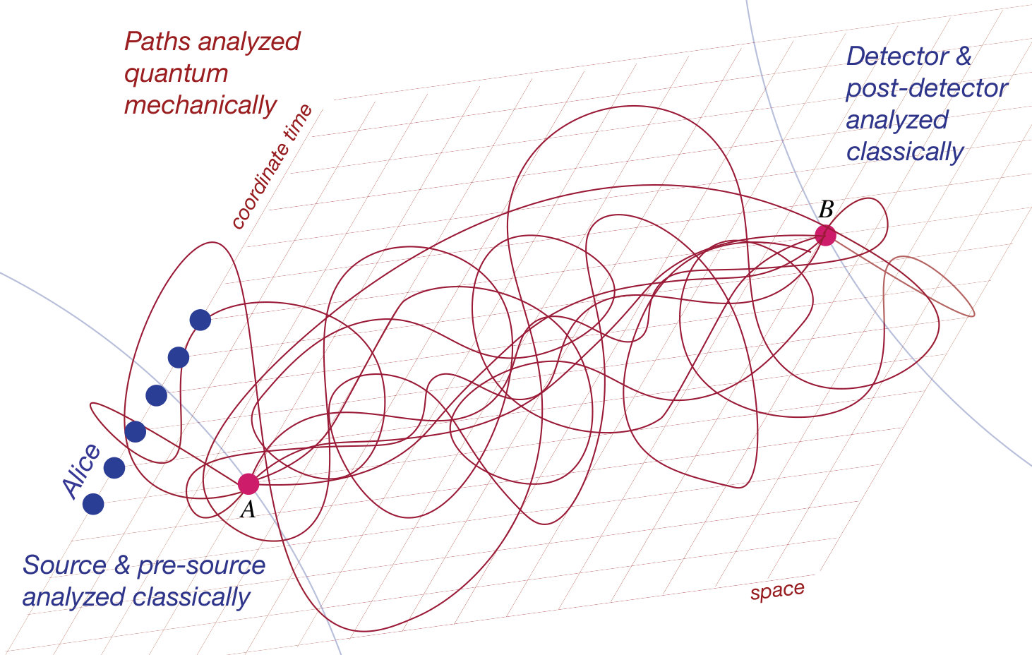 Figure 1
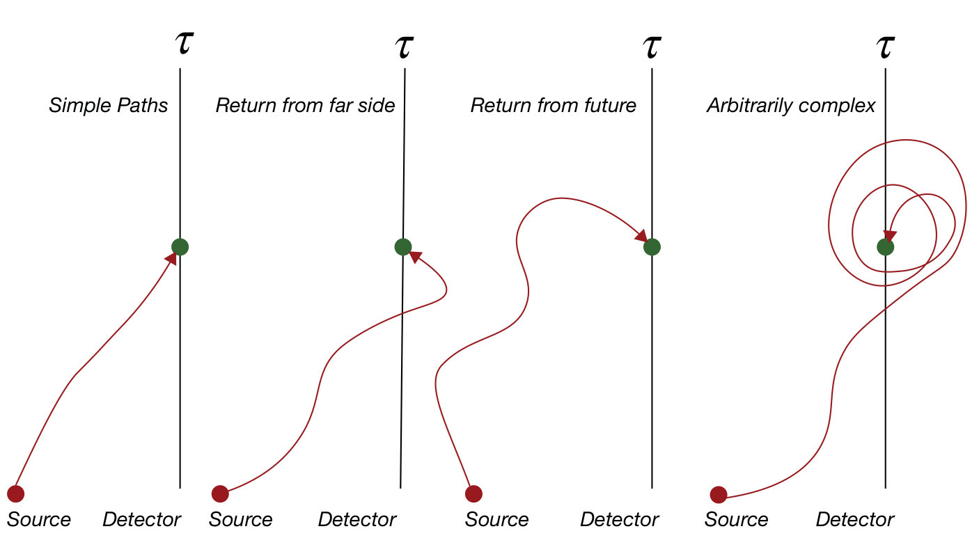 Figure 2
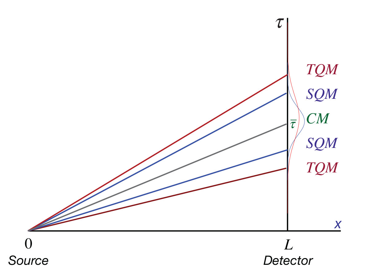 Figure 3
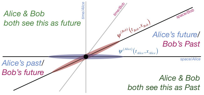 Figure 4
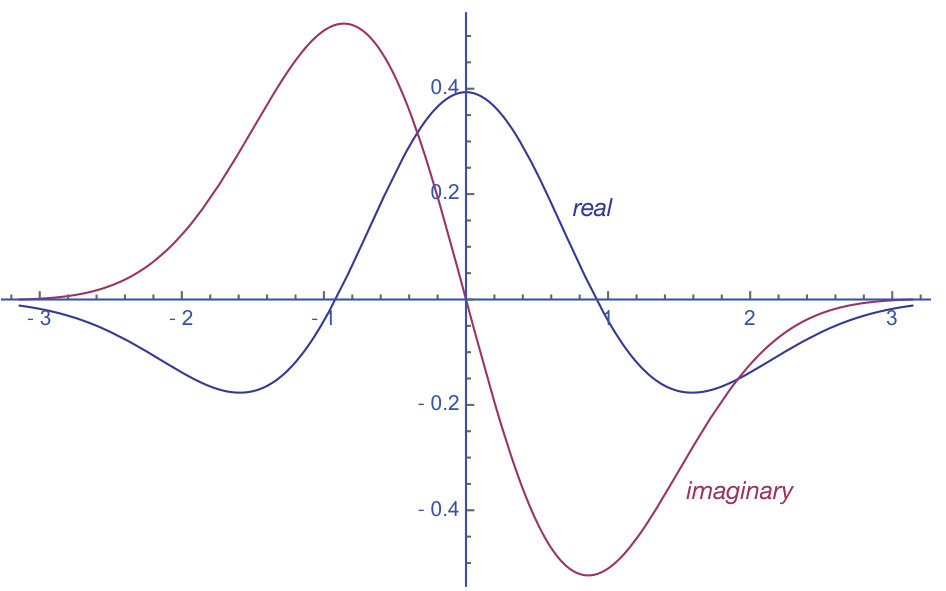 Figure 5
 Figure 6
 Figure 7
 Figure 8
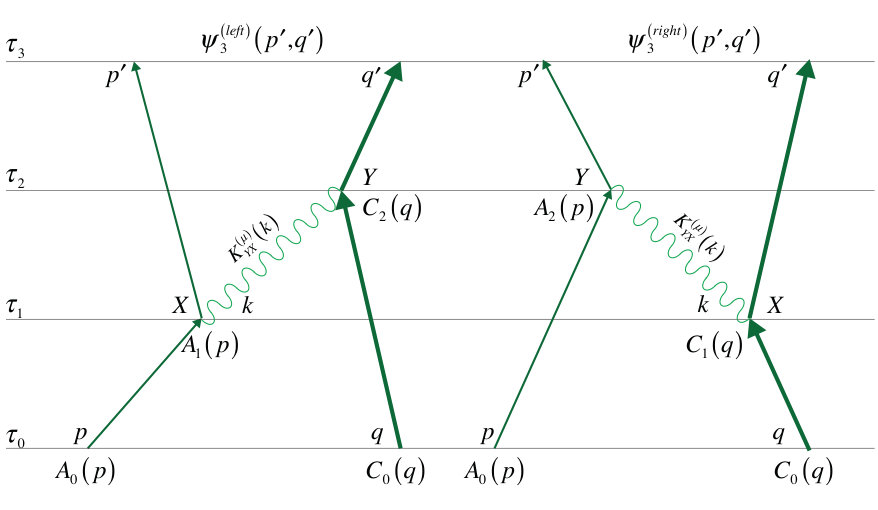 Figure 9
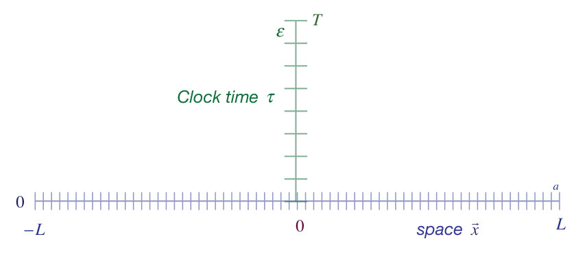 Figure 10
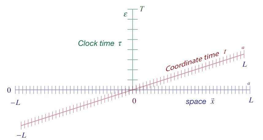 Figure 11
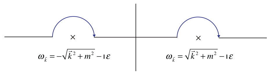 Figure 12
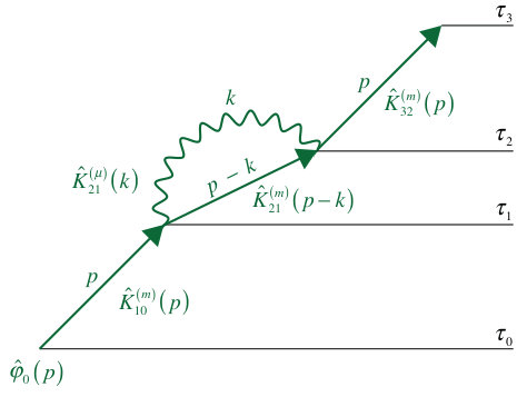 Figure 13
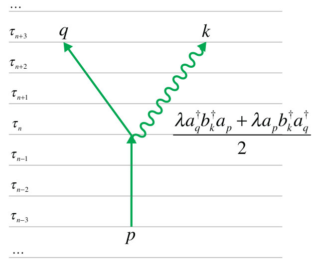 Figure 14
 Figure 15
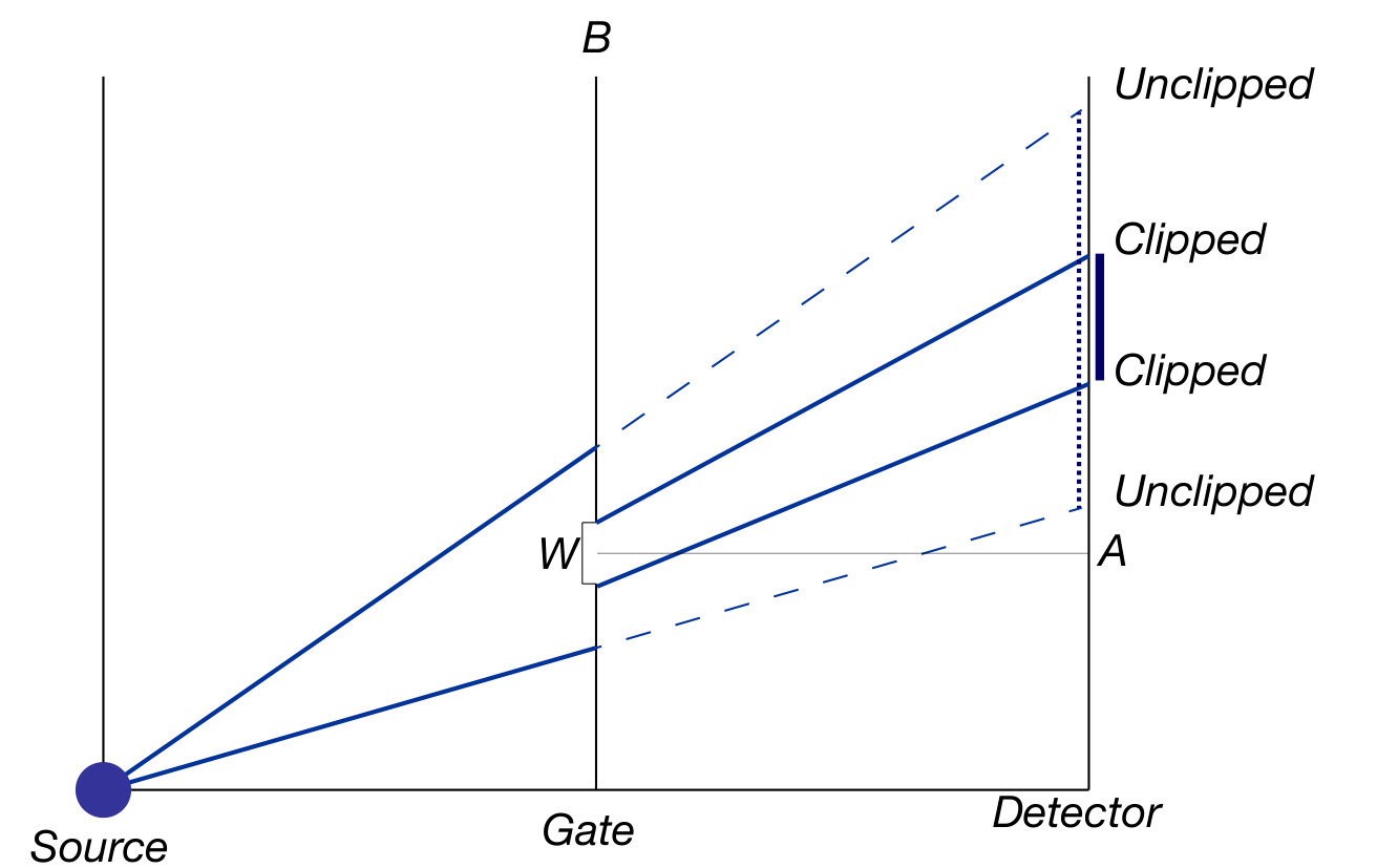 Figure 16
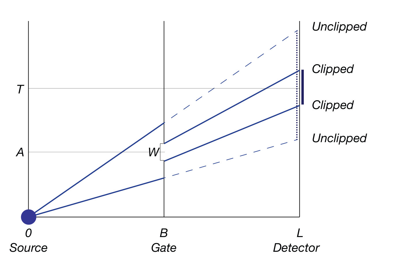 Figure 17
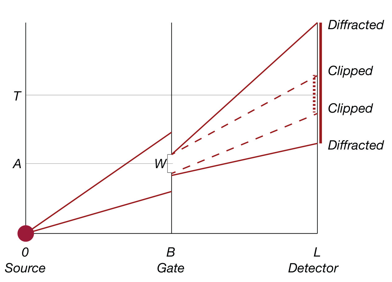 Figure 18
Peer Reviews
No public reviews on file for this paper yet. If you reviewed it on a platform where reviews are public (OpenReview, ICLR, NeurIPS, ICML), you can paste yours below so the community can read it here.
Videos
No videos yet. Explain this paper in a talk, walkthrough, or lecture? Add one.
Time dispersion in quantum mechanics
John Ashmead
Visiting Scholar, University of Pennsylvania, USA [email protected]
Abstract
In quantum mechanics the time dimension is treated as a parameter, while the three space dimensions are treated as observables. This assumption is both untested and inconsistent with relativity. From dimensional analysis, we expect quantum effects along the time axis to be of order an attosecond. Such effects are not ruled out by current experiments. But they are large enough to be detected with current technology, if sufficiently specific predictions can be made. To supply such we use path integrals. The only change required is to generalize the usual three dimensional paths to four. We predict a large variety of testable effects. The principal effects are additional dispersion in time and full equivalence of the time/energy uncertainty principle to the space/momentum one. Additional effects include interference, diffraction, and entanglement in time. The usual ultraviolet divergences do not appear: they are suppressed by a combination of dispersion in time and entanglement in time. The approach here has no free parameters; it is therefore falsifiable. As it treats time and space with complete symmetry and does not suffer from the ultraviolet divergences, it may provide a useful starting point for attacks on quantum gravity.
“Wheeler’s often unconventional vision of nature was grounded in reality through the principle of radical conservatism, which he acquired from Niels Bohr: Be conservative by sticking to well-established physical principles, but probe them by exposing their most radical conclusions.” – Kip Thorne [1].
“You can have as much junk in the guess as you like, provided that the consequences can be compared with experiment.” – Richard P. Feynman [2]
1 Introduction
1.1 Should the wave function extend in time as it does in space?
In relativity, time and space enter on a basis of formal equivalence. In special relativity, the time and space coordinates rotate into each other under Lorentz transformations. In general relativity, the time and the radial coordinate change places at the Schwarzschild radius (for instance in Adler [3]). In wormholes and other exotic solutions to general relativity, time can even curve back on itself as in Gödel or Thorne [4, 5].
But in quantum mechanics “time is a parameter not an operator” (Hilgevoord [6, 7]). This is clear in the Schrödinger equation:
[TABLE]
Here the wave function is indexed by time: if we know the wave function at time we can use this equation to compute the wave function at time . The wave function has in general non-zero dispersion in space, but is always treated as having zero dispersion in time. This would appear to be inconsistent with special relativity.
Consider Alice in her laboratory, her co-worker Bob jetting around like a fusion powered mosquito. Both are studying the same system but with respective wave functions:
[TABLE]
Alice and Bob center their respective wave functions on the particle:
[TABLE]
These are distinct wave functions but give the same predictions for all observables. And do so to an extremely high degree of reliability.
But at Alice’s time zero, Bob’s wave function extends into her past and future. And at Bob’s time zero her wave function extends into his past and future.
There are at least two problems here.
One is that in quantum mechanics there is a strict “plane of the present”. The quantum mechanical wave function is non-localized in space but is strictly localized in time. What if Alice decided to work with Bob’s wave function, rather than her own? She will get by hypothesis all the same predictions, but will be using a wave function that from her point of view slops into past and future.
The other is that from the point of view of special relativity, there should not be a strict “plane of the present” in the first place. We should be able to rotate between the four dimensional references frames of Alice and Bob as easily as we rotate between references frames for the three space dimensions.
What happens if we shift to four dimensional wave functions?
[TABLE]
Assume the coordinate systems for Alice and Bob are related by a Lorentz transformation :
[TABLE]
Then their wave functions can be related by a Lorentz transformation of their coordinates:
[TABLE]
and matters are much more straightforward.
We make this our basic hypothesis: the quantum mechanical wave function should be extended in the time direction on the same basis as it is extended along the three space dimensions.
We are playing a “game of if” here: we will push the idea as hard as we can and see what breaks. We are not going to argue that this is or is not true. We are going to look for experimental tests and then let the experimentalists decide the question.
There are two principal effects:
Dispersion in time appears on same basis as dispersion in space. Physical wave functions are always a bit spread out in space; they will now also be a bit spread out in time. 2. 2.
The uncertainty principle for time/energy is treated on same basis as the uncertainty principle for space/momentum. If a particle’s position in time is well-defined, its energy will highly uncertain and vice versa.
1.1.1 Dispersion in time
If the wave functions normally have an extension in time then every time-specific measurement should show additional dispersion in time.
Suppose we are measuring the time-of-arrival of a particle at a detector. Define the average time-of-arrival as:
[TABLE]
with an associated uncertainty:
[TABLE]
The probability distribution for the particle will normally be spread out in space, so its arrival times will also be spread out, depending on the velocity of the particle and its dispersion in space.
But if it also has a dispersion in time, then part of the wave function will reach the detector – thanks to the fuzziness in time – a bit sooner and also a bit later than otherwise expected. There will be an additional dispersion in the time-of-arrival due to the dispersion in time.
As we will see (subsection 4.3), at non-relativistic speeds, the dispersion in the time-of-arrival is dominated by the dispersion in space, so this effect may be hard to pick out. At relativistic speeds, the contributions of the space and time dispersions can be comparable.
1.1.2 Uncertainty principle for time and energy
Of particular significance for this work are differences in the treatment of the uncertainty principle for time/energy as opposed to that for space/momentum.
In the early days of quantum mechanics, these were treated on same basis. See for instance the discussions between Bohr and Einstein of the famous clock-in-a-box experiment [8] or the comments of Heisenberg in [9].
In later work this symmetry was lost. As Busch [10] puts it “… different types of time energy uncertainty can indeed be deduced in specific contexts, but … there is no unique universal relation that could stand on equal footing with the position-momentum uncertainty relation.” See also Pauli, Dirac, and Muga [11, 12, 13, 14].
There does not appear to be any experimental test of this or observational evidence for it; it is merely the way the field has developed.
That is not to say that there are not uncertainties with respect to time, but they are side effects of other uncertainties in quantum mechanics. For instance, if a particle is spread out in space, moving to the right, and going towards a detector at a fixed position, its time-of-arrival will have a dispersion in time. But this is a side-effect of the dispersion in space.
Now consider a particle going through a narrow slit in time, for instance a camera shutter. Its wave function will be clipped in time. If the wave function is not extended in time, then the wave function will merely be clipped: the resulting dispersion in time at detector will be reduced.
But if the wave function is extended in time and the Heisenberg uncertainty principle applies in time/energy on the same basis as with space/momentum, then an extremely fast camera shutter will give a small uncertainty in time at the gate:
[TABLE]
causing the uncertainty in energy to become arbitrarily great:
[TABLE]
which will in turn cause the wave function to be diffracted, to fan out in time, and the dispersion in time-of-arrival to become arbitrarily great.
1.1.3 A necessary hypothesis
This question does not appear to have been attacked directly. As noted, the assumption that the wave function is not extended in time seems to have crept into the literature of its own, without experimental test or observational evidence.
To make an experimental test of this question we have to develop predictions for both branches:
Assume the wave function is not extended in time. Make predictions about time-of-arrival and the like. 2. 2.
Assume the wave function is extended in time. Make equivalent predictions. 3. 3.
Compare.
We have to develop both branches in a way that makes the comparison straightforward.
Further, to make the results falsifiable we have to develop the extended-in-time branch in a way that is clearly correct. A null result should show that the wave function is not extended in time.
These objectives drive what follows.
1.1.4 Literature
The literature for special relativity and for quantum mechanics is vast. Our focus is on the critical intersection of the two. References of particular interest here include:
- •
Stueckelberg & Feynman’s original papers: [15, 16, 17, 18, 19, 20].
- •
Reviews of the role of time, Schulman, Zeh, Muga, Callender: [21, 22, 13, 14, 23].
- •
Block universe picture: Parmenides, Barbour, Price: [24, 25, 26].
- •
Cramer’s transactional interpretation: [27, 28, 29, 30].
- •
The time symmetric quantum mechanics of Aharonov and Reznik: [31, 32].
- •
The relativistic dynamics program of Horwitz, Piron, Land, Collins, and others: [33, 34, 35, 36, 37, 38, 39, 40]. This program is a natural outgrowth of Stueckelberg & Feynman’s work.
Our approach here may be understood as falling within the relativistic dynamics framework, but with the emphasis placed on the “coordinate time” rather than the “evolution parameter” aspects of that program. We will discuss this in detail once an appropriate foundation has been laid.
1.2 Order of magnitude estimate
Has this hypothesis has already been falsified? Quantum mechanics has been tested with extraordinary precision. Should associated effects have been seen already, even if not looked for?
Consider the atomic scale given by the Bohr radius . We take this as an estimate of the uncertainty in space.
We assume the maximum symmetry possible between time and space. We therefore infer that the uncertainty in time should be of order the uncertainty in space (in units where ).
Dividing the Bohr radius by the speed of light we get the Bohr radius in time , or less than an attosecond. is therefore our starting estimate of the uncertainty in time.
Therefore from strictly dimensional and symmetry arguments, the effects will be small, of order attoseconds. This is sufficient to explain why such effects have not been seen.
At the same time, the time scales we can look at experimentally are now getting down to the attosecond range. A recent paper by Ossiander et al [41] reports results at the sub-attosecond level.
Therefore if we can provide the experimentalists with a sufficiently well-defined target, the hypothesis should be falsifiable in practice.
1.3 Plan of attack
Look, I don’t care what your theory of time is. Just give me something I can prove wrong. – experimentalist at the 2009 Feynman Festival in Olomouc
1.3.1 Primary objective is falsifiability
It is not enough to extend quantum mechanics to include time. It is necessary to do so in a way that can be proved wrong. The approach has to be so strongly and clearly constrained that if it is proved wrong, the whole project of extending quantum mechanics to include time is falsified.
Our requirements are therefore that we have:
the most complete possible equivalence in the treatment of time and space – manifest covariance at every point at a minimum, 2. 2.
consistency with existing experimental and observation results, 3. 3.
and consistency between the single particle and multiple particle domains.
These requirements leave us with no free parameters. And having no free parameters means in turn that our hypothesis is falsifiable in principle.
To get to falsifiable in practice, we will look for the simplest cases that make a direct comparison possible.
We will also look at points of principle that need to be addressed, to ensure that the approach is not ruled out by, say, violations of unitarity.
We will use the acronym SQM for standard quantum mechanics. We will use the acronym TQM for temporal quantum mechanics. By TQM we mean SQM with time treated on the system basis as space: time just as much an observable as the three space dimensions.
We do not mean by “temporal quantum mechanics” that time itself comes in small chunks or quanta! For instance, there has been speculation that time is granular at the scale of the Planck time: . Maybe it is, maybe it isn’t. But as this is 25 orders of magnitude smaller than the times we are considering here, it is reasonable for us to take time as continuous. And since space is treated by SQM as continuous, and since the defining assumption of TQM is the maximum symmetry between time and space, we are required to take time in TQM continuous.
1.3.2 Extruding quantum mechanics in time
If you have worked with a CAD/CAM or 3D drawing program you are familiar with the “extrude” operation, where you take a circle or square and extrude it into the third dimension111See Abbott’s classic Flatland [42] for a delightful example.. That is all we are going to do here. We are going to use manifest covariance as the rule for going from three dimensions to four – so that is the invariant rather than – but the principle is the same.
The advantage is that with this approach we have no free parameters. The moment we introduce a free parameter we put falsifiability at risk since we are thereby creating a “fudge factor”. And any fudge factor might let us say “well perhaps no effect was seen at scale , but at smaller scale , then we shall see!”. We want our experimentalists to be able to say, “not seen, therefore not there!”
It might be that we should have done the extrude at a slight angle, extruding our circle into, say, an oblate or prolate spheroid rather than a perfect one. But this does not seriously impact falsifiability – such an oblate or prolate spheroid should still have the same overall scale of a Bohr radius in time, it will still give our experimentalist a fixed target. (We discuss possible meanings of “a slight angle” in subsection 3.5 and again in the discussion).
We will use path integrals as our defining formalism. With the path integral approach we can extrude the paths from three to four dimensions in a straightforward way, while leaving the rest of the machinery essentially untouched. With other formalisms, it is less clear what “extrude” means. But once we have the meaning of extrude worked out for path integrals, we can, as it were, rotate our path integral formalism into other formalisms, seeing what “extruding quantum mechanics in time” looks like as a Schrödinger equation or in quantum field theory.
Our plan:
1.3.3 Single particle case
In the single particle case we will:
Generalize path integrals to include time as an observable. 2. 2.
Derive the corresponding Schrödinger equation as the short time limit of the path integral. 3. 3.
Develop the free solutions. We will estimate the initial wave function, let it evolve in time, and detect it. We will compute the dispersions of time-of-arrival measurements in SQM and in TQM. In general the differences are real but small. 4. 4.
Analyze the single and double slit experiments. The single slit in time experiment provides the decisive test of temporal quantum mechanics. In SQM, the narrower the slit, the less the dispersion in subsequent time-of-arrival measurements. In TQM, the narrower the slit, the greater the dispersion in subsequent time-of-arrival measurements. In principle, the difference may be made arbitrarily great.
1.3.4 Multiple particle case
We will then extend TQM to include the multiple particle case, i.e. field theory. We will show, using a toy model, that:
We can extend the usual path integral approach to include time as an observable. The basis functions in Fock space extend in a natural way from three to four dimensions, the Lagrangian is unchanged, and the usual Feynman diagram expansions appear. 2. 2.
For each Feynman diagram in SQM we can compute the TQM equivalent. Therefore any problem that can be solved using Feynman diagrams in SQM can be solved in TQM. 3. 3.
The usual ultraviolet divergences do not appear (the combination of dispersion in time and entanglement in time contain them). 4. 4.
And that there are a large number of additional experimental effects to be seen, including:
- (a)
wave functions anti-symmetric in time, 2. (b)
correlations, entanglement, and interference in time, 3. (c)
and forces of anticipation and regret.
1.3.5 Overall conclusions
With this done, we will argue in the discussion:
that TQM is not ruled out a priori. 2. 2.
that TQM is falsifiable. And given experimental work like Ossiander’s, probably with current technology. 3. 3.
that TQM is a source of interesting experiments. Every foundational experiment in SQM has an “in time” variant. 4. 4.
that TQM is a potential starting point for attacks on the quantum gravity problem, since TQM is manifestly covariant and untroubled by the ultraviolet divergences. 5. 5.
that as TQM is a straight-forward extrapolation of quantum mechanics and special relativity, experiments that falsify TQM are likely to require modification of our understanding of either quantum mechanics or special relativity or both. Something will have to break.
1.3.6 Limits of the current investigation
We do no more here than is required to establish that TQM is well-defined, self-consistent, and falsifiable.
It will be clear from the development that the basic idea could be extended in a number of directions; we review some of these in the concluding discussion.
The conventions used in this work are spelled out in A.
2 Path integrals
2.1 Overview
To extend quantum mechanics to include time we will take as our starting point Feynman’s path integral approach to quantum mechanics [43, 44, 45, 46, 47, 48, 49, 50, 51, 52].
With the path integral approach, the only change we will need to make is to generalize the paths from varying in three dimensions to varying in four.
To make clear what this means, consider the case of Alice walking her dog, say from her front door to Bob’s.
Alice will take the shortest (classical) path from door to door.
But her dog will dart from side to side, now investigating a mailbox to the left, now checking out a lamppost to the right. In fact, as a quantum dog he will investigate all such paths simultaneously. While he will start at the same time and place as Alice, and finish at the same time and place as Alice, in between he will travel simultaneously along all possible paths.
But – in SQM – only along paths in space. At each tick of Alice’s digital watch, her dog will be found off to the left or right, jumping up or digging down, further along the path to Bob’s, or holding back for an important investigation.
But in TQM, the quantum dog can – and therefore will – advance into the future and drop back into the past. So that tick by tick of Alice’s watch, her dog’s paths will have to tracked in four dimensions rather than three.
This is harder to visualize, being out of our normal experience. So we develop the analysis a bit formally, letting math take the place of an as yet undeveloped intuition.
Path integrals, as the name suggests, are done by summing over all paths from starting point to finish, weighting each path by the integral of the Lagrangian (the action) along it:
[TABLE]
Piece by piece:
is the initial wave function. We will be breaking these down into sums over Gaussian test functions using Morlet wavelet analysis. 2. 2.
is the clock time as given by Alice’s digital watch. We will break up the paths into the bits from one clock tick to the next. 3. 3.
represents the paths. Each path is defined by its coordinates at each clock tick. In SQM, these are the values of at each clock tick. In TQM these are values of at each clock tick. 4. 4.
is a suitable Lagrangian. We will be using one that works equally well for both SQM and TQM. 5. 5.
is the action, the integral over the Lagrangian taken path by path. 6. 6.
And is the final wave function, the amplitude for the dog to arrive at Bob’s door step.
We will look at:
What do we mean by the clock time? 2. 2.
What do we mean by the coordinate time in ? 3. 3.
How do we define the initial wave function in a way that does not potentially bias the outcome? 4. 4.
What Lagrangian shall we use? 5. 5.
How do we get the sums to converge? 6. 6.
Having gotten the sums to converge, how do we normalize them? 7. 7.
And what do all the pieces look like when we put them back together?
2.2 Laboratory time
We consider the action, the integral of the Lagrangian over time:
[TABLE]
In classical mechanics, we are free to take the parameter as any monotonically increasing variable. We will get the same classical equations of motion in any case.
A typical choice is to select as the proper time of the particle in question. However this makes it difficult to extend the work to the multiple particle case, where there are many particles and therefore many proper times in play.
Here we choose to use the time as shown on a laboratory clock. We take the term laboratory time from Busch [10]. We will use the terms clock time and laboratory time interchangeably.
It is useful to visualize this clock as a metronome, breaking up the clock time into a series of ticks each of length . If at the source, and at the detector, we have:
[TABLE]
We will take the limit as as the final step in the calculation.
2.3 Coordinate time
We visualize a four dimensional coordinate system coordinates . We will refer to as coordinate time by analogy with the three coordinate space dimensions: coordinate , coordinate , and coordinate .
Paths are defined with reference to this coordinate system. If the time by Alice’s watch is , then each path will have a location at given by:
[TABLE]
It may help to think of the coordinates as laid out on a piece of four dimensional graph paper. At a specific clock tick , a specific path will be represented by a dot on a specific vertex on the four dimensional graph paper. If we want to see the progress of the path with respect to clock time, we can flip the series of pieces of graph paper like one of those old time flip movies.
If our graph paper has grid lines in each direction, the number of vertices on a page is , and the number of paths total is . Each different sequence of grid points counts as a distinct path.
The path integral measure is usually defined by assigning a weight of one to each distinct path, and then taking the limit as the spacing goes to zero.
Since coordinate time is on the same footing as the three space coordinates it has a corresponding energy operator:
[TABLE]
We will refer to this as coordinate energy. It is not positive definite or bounded from below. Since can be positive or negative, by our controlling requirement of covariance can be positive or negative.
We discuss the relationship between clock time and coordinate time in F.
2.4 Initial wave function
We need a starting set of wave functions at clock time . We will need wave functions that extend in both coordinate time and space. The usual choices would be functions or plane waves.
In coordinate time these might be:
[TABLE]
[TABLE]
or in space:
[TABLE]
[TABLE]
But neither functions nor plane waves are physical. Their use creates a risk of artifacts.
More physical would be Gaussian test functions, for instance in coordinate time:
[TABLE]
or in space:
[TABLE]
But while Gaussian test functions are physically reasonable they are not completely general.
We can achieve both generality and physical reasonableness by using a basis of Morlet wavelets [53, 54, 55, 56, 57, 58, 59, 60, 61, 62].
Morlet wavelets are derived by starting with a “mother” wavelet:
[TABLE]
and scaling and displacing it with the replacement :
[TABLE]
Any normalizable function can be broken up into wavelet components using:
[TABLE]
And then recovered using the inverse Morlet wavelet transform:
[TABLE]
The value of is worked out in [62].
Therefore we can write any physically reasonable wave function in time in terms of Morlet wavelets.
We may include space by using products of Morlet wavelets:
[TABLE]
Clearly it would be cumbersome to track four dimensional Morlet wavelets at every step.
Fortunately we do not need to perform the Morlet wavelet analyses; we merely need the ability to do so. As each Morlet wavelet may be written as a sum of a pair of Gaussians, Morlet wavelet analysis lets us write any physically reasonable wave function as a sum over Gaussians. Provided we are dealing only with linear operations – the case throughout here – we can work directly with Gaussian test functions. By Morlet wavelet analysis the results will then be valid for any physically reasonable wave functions.
2.5 Lagrangian
To sum over the paths – to construct the path integral – we will need to weight each path by the exponential of the action, where the action is defined as the integral of the Lagrangian over the laboratory time:
[TABLE]
We require a Lagrangian which:
Is manifestly covariant, 2. 2.
Produces the correct classical equations of motion, 3. 3.
And gives the correct Schrödinger equation.
We would further prefer a Lagrangian which is the same for both SQM and TQM. This will let us argue that we are treating SQM and TQM with the most complete possible equality.
Somewhat surprisingly such a Lagrangian exists. In Goldstein’s well-known text on classical mechanics [63] we find:
[TABLE]
The potentials are not themselves functions of the laboratory time . The mass is the rest mass of the particle, an invariant.
This Lagrangian is unusual in that it uses four independent variables (the usual three space coordinates plus a time variable) but still gives the familiar classical equations of motion (see B).
This Lagrangian therefore provides a natural bridge from a three to a four dimensional picture.
The classical equations of motion are still produced if we add a dimensionless scale and an additive constant to the Lagrangian:
[TABLE]
The Lagrangian is therefore only determined up to and . The requirement that we match the SQM results will fix and (subsection 3.3).
2.6 Convergence
How do we get the integrals over the paths to converge without breaking covariance?
We compute the path integral for the kernel by slicing the clock time into an infinite number of intervals and integrating over each:
[TABLE]
with an appropriate normalization factor.
Consider the discrete form of the Lagrangian. We use a tilde to mark the coordinate time part and an overbar to mark the space part:
[TABLE]
[TABLE]
[TABLE]
[TABLE]
We are using the mid-point rule, averaging the scalar and the vector potentials over the start and end points of the step, by analogy with the rule for three dimensions (Schulman [44], Grosche and Steiner [49]).
Now look at a single step for the free case, vector potential zero:
[TABLE]
The formal tricks normally used to ensure convergence do not work here (e.g. Kashiwa or Zinn-Justin [48, 50]). Perhaps the most popular of these is the use of Wick rotation to shift to a Euclidean time:
[TABLE]
This causes integrals to converge rapidly going into the future, but makes the past inaccessible. For instance, factors of – which spring up everywhere in path integrals – converge going into the future, but blow up going into the past. If we are to treat time on the same footing as space – our central assumption – then past and future must be treated as symmetrically as left and right.
Another approach is to add a small convergence factor at a cleverly chosen spot in the arguments of the exponentials. But if we attach a convergence factor to and separately, we break manifest covariance. If we attach our convergence factor to both, the fact that the and parts enter with opposite sign means any convergence factor that works for one will fail for the other. We could try attaching one to the mass , but this also fails. For instance if and we subtract a small factor of from the mass:
[TABLE]
the integral converges but the integral diverges.
We recall the kernel has meaning only when applied to a specific physical wave function. If we break the incoming wave up into Morlet wavelets and then into Gaussian test functions, we see that each integral converges by inspection, the factor ensures this.
So for physically significant wave functions, there is no problem in the first place. Effectively we are taking seriously the point that the path integral kernel is a distribution, only meaningful with respect to specific wave functions.
2.7 Normalization
Now that we have our path integrals converging, we have to normalize them. If we start from the Schrödinger equation, the normalization is wired in. But in path integrals we are a bit at sea.
We will here deal with the free case, verifying the normalization is correct in the general case in C.
The normalization factor for steps we will call . The defining requirement is that, if the initial wave function is normalized to one, then with the inclusion of , the final wave function will be normalized to one as well:
[TABLE]
If depends on the particular , then we have failed.
We now compute the factor of .
2.7.1 Normalization in time
We start with the coordinate time dimension only. Consider a Gaussian test function centered on an initial position in coordinate time :
[TABLE]
We write the kernel for the time part as:
[TABLE]
The wave function after the initial integral over is:
[TABLE]
or:
[TABLE]
with the dispersion factor .
The normalization requirement is:
[TABLE]
The first step normalization is correct if we multiply the kernel by a factor of . Since this normalization factor does not depend on the laboratory time the overall normalization for infinitesimal kernels is the product of of these factors:
[TABLE]
Note also that the normalization does not depend on the specifics of the Gaussian test function (the values of , , and ) so it is valid for an arbitrary sum of Gaussian test functions as well. And therefore, by Morlet wavelet decomposition, for an arbitrary wave function.
As noted, the phase is arbitrary. If we were working the other way, from Schrödinger equation to path integral, the phase would be determined by the Schrödinger equation itself. The specific phase choice we are making here has been chosen to help ensure the four dimensional Schrödinger equation is manifestly covariant, see below. We may think of the phase choice as a choice of gauge (see D).
Therefore the expression for the free kernel in coordinate time is (with , ):
[TABLE]
Doing the integrals we get:
[TABLE]
and free wave functions in coordinate time:
[TABLE]
2.7.2 Normalization in space
We redo the analysis for coordinate time for space. We use the correspondences:
[TABLE]
With these we can write down the equivalent set of results by inspection. Since we will need the results below, we do this explicitly. We get the initial Gaussian test function:
[TABLE]
free kernel:
[TABLE]
and normalized kernel:
[TABLE]
The kernel matches the usual (non-relativistic) kernel [64, 44] if .
The wave function is:
[TABLE]
with the definition of the dispersion factor parallel to that for coordinate time (but with opposite sign for the imaginary part).
2.7.3 Normalization in time and space
The full kernel is the product of the coordinate time kernel, the three space kernels, and the constant term . We understand to refer to coordinate time and all three space dimensions:
[TABLE]
We have done the analysis only for Gaussian test functions, but by Morlet wavelet decomposition it is completely general.
2.8 Formal expression
We now have the full path integral:
[TABLE]
with the measure:
[TABLE]
and the discretized Lagrangian at each step:
[TABLE]
We will show that in the next section.
3 Schrödinger equation
3.1 Overview
The path integral and Schrödinger equation views are complementary. We need both to fully understand either.
We derive the Schrödinger equation from the path integral by taking the short time limit of the path integral form.
By comparing the result to the Klein-Gordon equation – and making a reasonable assumption about the long time evolution of the wave functions – we are able to fix the additive and scale constants in the Lagrangian.
The resulting equation looks like the Klein-Gordon equation over short times but shows some drift over longer times. We use some heuristic arguments to estimate the scale of the long term drift as of order picoseconds, a million times longer than the attosecond scale of the time dispersions we are primarily concerned with here. We will therefore be able to largely ignore this drift.
With defined, we look at a further problem. We have done the derivation of path integral and Schrödinger equation forms from Alice’s perspective. But what of Bob, jetting around like a fusion powered mosquito?
We resolve this conflict by arguing that we can find a natural rest frame that both can use. Starting with an argument of Weinberg’s, we argue we can associate an energy-momentum tensor with spacetime. This means we can associate a local rest frame with spacetime. And this local rest frame can provide the neutral and agreed defining frame for TQM.
This will complete the formal development of TQM.
Before turning to applications, we will then look at the relationship of TQM to the relativistic dynamics program. We will argue that TQM may be understood as a member of that program aggressively specialized to achieve falsifiability.
3.2 Derivation of the Schrödinger equation
Normally the path integral expression is derived from the Schrödinger equation. But because for us the path integral provides the defining formulation we need to run the analysis in the “wrong” direction.
Our starting point is a derivation of the path integral from the Schrödinger equation by Schulman [44]. We run his derivation in reverse and with one extra dimension222This derivation is done for the free case in Fanchi [36]. .
We start with the discrete form of the path integral. We consider a single step of length , taking at the end. Because of this, only terms first order in are needed.
Following Schulman, we define the coordinate difference:
[TABLE]
We rewrite the functions of as functions of and . We expand the vector potential:
[TABLE]
and the wave function:
[TABLE]
giving:
[TABLE]
We now expand in powers of . We do not need more than the second power:
[TABLE]
The term zeroth order in gives:
[TABLE]
This is not surprising; the normalization above was chosen to do this.
Terms linear in give zero when integrated.
The terms second order in (first in ) are:
[TABLE]
Integrals over off-diagonal powers of order give zero. Integrals over diagonal terms give:
[TABLE]
The expression for the wave function is therefore:
[TABLE]
Taking the limit and multiplying by , we get the Schrödinger equation for TQM:
[TABLE]
or:
[TABLE]
If we make the customary identifications , or we have:
[TABLE]
3.3 Long, slow approximation
We can now fix the scale and additive constants by looking at the behavior of the Schrödinger equation over longer times.
In his development of quantum mechanics from a time-dependent perspective [65], Tannor used a requirement of constructive interference in time to derive the Bohr condition for the allowed atomic orbitals. We use a similar approach here.
If we average over a sufficiently long period of time, the results will be dominated by the components with:
[TABLE]
The argument here is not that the typical variation from the long, slow solution is small, but rather that over time interactions with the system in question will tend to be dominated by interactions with the stabler, slower moving components. Interactions with more rapidly varying components will tend to average to zero.
Accepting this, then the right side looks like the Klein-Gordon equation. To complete this identification, first look at the case with the vector potential zero:
[TABLE]
Now when is not zero we have:
[TABLE]
We will refer to this as the “long, slow approximation”.
In the free case, the long, slow approximation picks out the on-shell components:
[TABLE]
And more generally the solutions of the Klein-Gordon equation with the minimal substitution :
[TABLE]
The two constants are now fixed. The full Schrödinger equation is:
[TABLE]
and in momentum space:
[TABLE]
The free Schrödinger equation is:
[TABLE]
and in momentum space:
[TABLE]
We establish in C this equation is unitary. Therefore if a wave function is normalized at :
[TABLE]
then at any later clock time we will have:
[TABLE]
We next estimate the time scales over which we expect the long, slow approximation to be valid.
3.4 How long and how slow?
We have argued that we can fix the scaling and additive constants by looking at the behavior of the Schrödinger equation over long times. What do we mean by long times?
To see the relevant scale, we estimate the clock frequency :
[TABLE]
In the non-relativistic case is of order mass plus kinetic energy:
[TABLE]
So we have:
[TABLE]
This is just the kinetic energy, squared. In an atom the kinetic energy is of order the binding energy:
[TABLE]
So the numerator is of order squared. But the denominator is of order . So we can estimate the clock frequency as:
[TABLE]
Energies of millionths of an electron volt correspond to times of order millions of attoseconds or picoseconds, a million times longer than the natural time scale of the effects we are looking at. So the long, slow approximation is reasonable.
The physical picture that emerges is of a particle that is extended in time on the same basis as space, with its wave function extend in all four dimensions, and – if we think in terms of path integrals – the associated paths wandering around in all four dimensions, not just the traditional three.
It may be amusing to note that from this perspective there is no such thing as an onshell particle; in momentum space the onshell part of the wave function is always a set of measure zero. It is only over scales of picoseconds and greater that an onshell description of the particle may give an acceptable approximation.
3.5 Observer independent choice of frame
There remains one piece of the puzzle; we need to establish that the use of the clock time does not itself violate covariance.
If we did the above derivation for Bob rather than Alice, we would see Alice’s clock time replaced by Bob’s clock time () where is his velocity relative to her.
We therefore have one free parameter left to fix before we can declare our analysis free of free parameters.
If Bob is not going that quickly (relative to Alice) the errors created by ambiguities with respect to will introduce only small corrections; of only second order and therefore not relevant for falsifiability.
Even if we were prepared to accept that, establishing frame independence is interesting as a point of principle.
This may be done in a natural way by making use of an observation from Weinberg [66]. Per Weinberg, we may treat the Einstein field equation for general relativity as representing conservation of energy-momentum when exchanges of energy momentum with spacetime are included.
Consider the Einstein field equations:
[TABLE]
Rewrite as:
[TABLE]
We may use this to associate an energy momentum tensor ( in Weinberg’s notation) with local space time. Define:
[TABLE]
where vanishes at infinity but is not assumed small. The part of the Ricci tensor linear in is:
[TABLE]
The exact Einstein equations may be written as:
[TABLE]
where is defined by:
[TABLE]
Weinberg then argues we may interpret as the energy-momentum of the gravitational field itself.
Accepting this, we change to a coordinate frame in which is diagonalized. We will refer to this as the rest frame of the vacuum or the frame. We can treat this frame as the defining frame for the four dimensional Schrödinger equation. As the frame is invariant (up to rotations in three-space) we now have an invariant definition of the four dimensional Schrödinger equation.
This is obviously going to be a free-falling frame. So Alice and Bob – if they are working in a terrestrial laboratory – will have to adjust their calculations to include a correction for the upwards force the laboratory floor exerts against them. If their colleague Vera is working in an orbiting laboratory, she will be able to calculate without correction.
Here after, unless stated to contrary, we will assume we are working in the “rest frame of the vacuum”.
3.6 Relationship between TQM and the Relativistic Dynamics program
“In other words, we are trying to prove ourselves wrong as quickly as possible, because only in that way can we find progress.” – Richard P. Feynman [2]
We have now fully defined the path integral expression and the Schrödinger equation.
It is appropriate therefore to pause to look at relationship of TQM to the relativistic dynamics program. (A helpful overview of the relativistic dynamics program is provided in Fanchi [35]).
3.6.1 TQM as part of the Relativistic Dynamics program
We start with Feynman [17], who uses the Lagrangian:
[TABLE]
giving:
[TABLE]
However with this approach, as Feynman notes, each particle would need its own evolution parameter . This would make extension to the multiple particle case problematic.
There are many variations on this in the literature. Fanchi [36] derives:
[TABLE]
This differs from Feynman’s by a factor of . Fanchi’s evolution parameter is for all practical purposes the negative of our clock time .
Land and Horwitz [37] give:
[TABLE]
This is Fanchi’s with the addition of the , a gauge term.
If we take and make the choice of gauge (see D):
[TABLE]
we get:
[TABLE]
which is the same as our Schrödinger equation (equation 74).
At this point we may argue that as the right hand-side is the Klein-Gordon equation, and the Klein-Gordon equation is strongly confirmed by experimental evidence we have:
[TABLE]
So the combination of the mass gauge () and the comparison with the Klein-Gordon equation give us the long slow approximation.
We have therefore placed our Schrödinger equation within the context of the relativistic program. This will let us use results from that program in the appropriate limit.
3.6.2 TQM and falsifiability
TQM may be thought of as a specialization of the relativistic dynamics program aimed at making the hypothesis “time should be treated on the same basis as space in quantum mechanics” falsifiable. This means in turn that we have to be able to rule out the class of such theories, not just one in particular.
To do this we need to extend quantum mechanics to include time in a way that depends only on covariance. We can admit no free or adjustable parameters; any such risk falsifiability.
We may understand each step of the program here from this point of view.
We used clock time as the “evolution parameter”. This is defined operationally – by the laboratory clock – and therefore introduces no free parameters. 2. 2.
We used path integrals as the defining representation; with these the only change we need to make is to have the paths extend in four rather than three dimensions. 3. 3.
We could not use plane waves or delta functions as the initial wave functions: as they are not physical, they introduce the risk of inducing mathematical artifacts and again threatening falsifiability. 4. 4.
We needed to treat general wave functions, not just a specialized subset. Otherwise the results might be conditional on the subset chosen. 5. 5.
We needed to ensure that our path integrals are convergent without the use of tricks. Otherwise the tricks can bring the results into question. The use of Morlet wavelet decomposition solved this and the previous two problems. 6. 6.
The resulting Schrödinger equation depends on the clock time. To eliminate such dependence (to lowest order) we showed that the time scales associated with the clock time are of order picoseconds, while the scales associated with dispersion in time are of order attoseconds – a million times smaller. So long as we work at the attosecond scale we should be able to ignore effects associated with clock time. 7. 7.
The clock time in turn depends on the choice of the laboratory frame. To further control for effects of the specific choice of laboratory frame, we showed we can define an invariant frame (the “rest frame of the vacuum”). By defining all calculations with reference to this invariant frame we eliminate the dependence of the clock time on the choice of a specific laboratory frame.
While we have fully defined the path integral expression and the Schrödinger equation, there are still some further questions that need to be addressed if we are to achieve falsifiability:
How do we estimate the initial wave functions in time in a robust and frame independent way (subsection 4.1)? 2. 2.
How do we understand the evolution of the wave function with respect to clock time: with the long, slow approximation we appear to be saying the wave function is frozen in time, that , which is clearly far from the case (subsection 4.2)? 3. 3.
How do we define the rules for detection in a way which is manifestly covariant (subsection 4.3)? 4. 4.
How do we produce at least one experiment with which we can unambiguously show that the wave function should not be extended in time (section 5)? 5. 5.
Realistic experiments will need to run at ultra-short times and therefore high energies. At these energies, particles may spring into existence from the vacuum. How do we extend this analysis to the multiple particle case in a way which is consistent with the work done in the single particle case (section 6)?
At attosecond times, we expect that the effects of dispersion in time will dominate. Over picosecond and longer times we expect that the effects of the clock time will need to be included.
Therefore, at attosecond times, we expect TQM will function as a kind of lowest common denominator for the relativistic dynamics program. At picosecond times, we may need to include contributions from the evolution parameter and therefore be able to discriminate among various branches of the relativistic dynamics program.
4 Free solutions
We now have the Schrödinger equation. What do its free solutions look like?
We examine in turn the birth, life, and death of a free particle. The calculations are straightforward. But each stage will present problems specific to TQM.
For convenience, we assemble the solutions of the free Schrödinger’s equation in E.
4.1 Initial wave function
What do our wave functions look like at start?
We have a chicken and egg problem here. Any initial wave function had itself to come from somewhere. How can we estimate the initial wave functions without first knowing them?
We look specifically at the Klein-Gordon equation for a static electric potential with no magnetic field:
[TABLE]
with potential:
[TABLE]
This includes attractive potentials, scattering potentials, and the free case as the special case when .
In SQM the Klein-Gordon equation is:
[TABLE]
In TQM the equivalent is the four dimensional Schrödinger equation:
[TABLE]
The long, slow approximation picks out the solutions with:
[TABLE]
We will assume we are already in possession of solutions to the SQM version of the problem:
[TABLE]
This is necessarily in a specific frame, since SQM solutions are always (from our perspective) taken with reference to a specific frame.
We leverage the SQM solutions in two different ways333This problem is also solved in Fanchi [36], using different methods. to get the TQM solution:
Separation of variables. Each SQM solution induces a TQM solution, which is the SQM solution with a plane wave bolted on. This is technically correct, but unphysical. 2. 2.
*Maximum entropy. *We can use the long, slow approximation to estimate the mean and uncertainty of the coordinate energy. With these we can use the method of Lagrange multipliers to get the maximum entropy solution. Maximum entropy solutions tend to be robust: even if we are wrong about the details, the order of magnitude should be correct. This will provide our preferred starting point.
As a quick check on the sanity of all this we will use the virial theorem to estimate the TQM version of the atomic wave functions. The width in time/energy of these matches the initial order of magnitude estimate we gave in the introduction.
We will also show that while we have chosen a specific frame in which to estimate the dispersion in time/energy we can get the estimate in an invariant way.
4.1.1 Solution by separation of variables
We solve the TQM Klein-Gordon equation using separation of variables, looking for solutions of the form:
[TABLE]
where is a solution of the SQM Klein-Gordon equation:
[TABLE]
Then the coordinate time part is:
[TABLE]
Because the potential is constant in time each use of the operator turns into a constant via:
[TABLE]
We get immediately:
[TABLE]
So every solution of the Klein-Gordon equation in SQM generates a corresponding solution in TQM.
We could accomplish the same thing, formally, by taking . Since we expect in general that (discussed further in the next section) this will often a give reasonable first approximation.
However this is not entirely satisfactory. We have a solution which is “fuzzy” in space, but “crisp” in time. A more realistic, if more complex solution, would include off-shell components. Even if our wave function started out as a simple plane wave in time, internal decoherence would rapidly turn it into something a bit more cloud-like. While mathematically acceptable, our solution is not physically plausible.
4.1.2 Solution by maximum entropy
The long, slow approximation picks out a single solution. But in practice we expect there would be a great number of solutions, with the one given by the long slow approximation merely the most typical.
Such a sum will have an associated probability density function. We can get a reasonable first estimate of this by defining appropriate constraints and then using the method of Lagrange multipliers to pick out the distribution with maximum entropy.
From the probability density, we will infer the wave function.
Estimate of the probability density
We start with the free case, as representing the simplest case of a constant potential. We treat the bound case below.
We assume we are given the SQM wave function in three dimensions. We use this to compute the expectation of the energy, and the expectation of the energy squared. These give us our constraints:
[TABLE]
The uncertainty in energy is defined as:
[TABLE]
The expectations are defined as integrals over the probability density:
[TABLE]
The constraints imply .
We will work with box normalized energy eigenfunctions:
[TABLE]
[TABLE]
Here is an integer running from negative infinity to positive and the eigenfunctions are confined to a box extending seconds into the future and seconds into the past, where is much larger than any time of interest to us. (We will use a similar approach in developing the four dimensional Fock space below, subsection 6.3.2).
A general wave function can be written as:
[TABLE]
The coefficients only appear as the square:
[TABLE]
Expressed in this language we have the constraints:
[TABLE]
We would like to find the solution that maximizes the entropy:
[TABLE]
We form the Lagrangian from the sum of the entropy and the constraints, with Lagrange multipliers , , and :
[TABLE]
To locate the configuration of maximum entropy, we take the derivative with respect to the :
[TABLE]
getting:
[TABLE]
Therefore the distribution of the is given by an exponential with zeroth, first, and second powers of the energy:
[TABLE]
The constraints force the constants:
[TABLE]
Estimate of the wave function
We therefore have the probability density in energy; now we wish to estimate the corresponding wave function in energy (or equivalently time).
The simplest – and therefore best – way to do this is to write the total wave function as the direct product of a wave function in energy times the postulated wave function in momentum:
[TABLE]
We then use the Gaussian test function that matches the derived density function for the energy factor:
[TABLE]
with values:
[TABLE]
and:
[TABLE]
Taking the Fourier transform of the energy part we have:
[TABLE]
[TABLE]
We set as the overall phase is already supplied by the space/momentum part.
The full wave functions are the products of the coordinate time and space (or energy and momentum) parts:
[TABLE]
[TABLE]
4.1.3 Bound state wave functions
We extend this approach to estimate the dispersion of a bound wave function in time.
In the case of a Coulomb potential we can estimate from the virial theorem:
[TABLE]
which implies:
[TABLE]
Since the average momentum is zero, we have the estimate of the uncertainty in energy as:
[TABLE]
Substituting the mass of the electron and the Rydberg constant, we have for the hydrogen ground state:
[TABLE]
And the corresponding dispersion in coordinate time is:
[TABLE]
This matches the order of magnitude estimate we started with (subsection 1.2). The numerical closeness is coincidental, but does increase confidence the order of magnitude is correct.
We have therefore as the initial estimate of the TQM wave function for a hydrogen atom:
[TABLE]
4.1.4 Frame independence of the estimate
We have given a reasonable estimate of the initial wave function in time/energy. However, we have not yet established that the estimate is independent of the initial choice of frame.
For both the bound and free cases, we choose our initial frame as the rest frame. We make our estimate, via maximum entropy in this frame, then to get the wave function in a arbitrary frame Lorentz transform to that frame:
[TABLE]
Since the rest frame is an invariant, the resulting initial wave functions are well-defined.
4.2 Evolution of the free wave function
Now that we know what our starting wave functions look like, how do they evolve over time?
For a first examination we work with the non-relativistic case; we will extend to the relativistic case below (section 6). We will first look at the SQM case, then the TQM case, then compare the two.
4.2.1 Evolution in SQM
We start with the familiar problem of the evolution of the non-relativistic wave function with respect to clock time. We work with two dimensions – – since the extension to is straightforward.
The non-relativistic Schrödinger equation is:
[TABLE]
At clock time zero we start with a Gaussian test function in momentum with average position , average momentum , and dispersion in momentum . To reduce clutter we use for :
[TABLE]
In momentum space the problem is trivial. The solution is:
[TABLE]
In coordinate space we get:
[TABLE]
with:
[TABLE]
[TABLE]
4.2.2 Evolution in TQM
In two dimensions the Schrödinger equation for TQM is:
[TABLE]
We start in energy momentum space. The momentum part is as above. We start with a Gaussian test function in energy, with average time at start , average energy , and dispersion in energy :
[TABLE]
Usually we will take .
As a function of clock time we get:
[TABLE]
We divide up the pieces of the clock time part, assigning the to the energy part, the to the momentum part, and keeping the third part outside:
[TABLE]
Now the energy part works in parallel to the momentum part:
[TABLE]
And in coordinate space:
[TABLE]
with the usual ancillary definitions:
[TABLE]
[TABLE]
and with the expectation for coordinate time:
[TABLE]
implying a velocity for coordinate time with respect to laboratory time:
[TABLE]
In the non-relativistic case, . So the expectation of the coordinate time advances at the traditional one-second-per-second rate relative to the clock time.
4.2.3 Comparison of TQM to SQM
The TQM and SQM approaches develop in close parallel. In both, the wave functions are centered on the classical trajectory as given by the solution of the Euler-Lagrange equations.
There is however one peculiarity.
We are relying on the long, slow approximation. Especially over short times, this means that the total wave function appears to be relatively static with respect to evolution in clock time:
[TABLE]
In momentum space:
[TABLE]
However, real wave functions are not static with respect to clock time.
The resolution is that most of the clock time dependence is carried by the coordinate time:
[TABLE]
And in the non-relativistic case we have:
[TABLE]
So we get as a rough approximation:
[TABLE]
We see that the expectation of the coordinate time is about equal to the clock time. While Alice’s dog is always getting ahead of and behind her, on average his position is about equal to hers:
[TABLE]
The Schrödinger equation gives the partial derivative with respect to clock time; the total derivative behaves as expected.
4.3 Time of arrival measurements
So we know what our wave function looks like at start and how it evolves with time. To complete the analysis of the free case we look at how it is detected.
We look specifically at the measurement of time-of-arrival. We assume we have a particle going left to right, starting at . We place a detector at position . It records when it detects the particle. The metric we are primarily interested in is the dispersion in time-of-arrival at the detector.
In SQM, if a detector located at position registers a hit by a particle we take the particle’s position in space as also . Therefore in TQM, if detector active at laboratory time registers a hit by a particle we must take the particle’s position in time as . This is required by our principle of maximum symmetry between time and space.
By the same token, in SQM if an emitter located at position emits a particle, we take the start position of the path as . Therefore in TQM, if an emitter active at laboratory time emits a particle, we must take the start position in coordinate time as .
In a practical treatment we would replace the phrases “at X” or “at T” with “within the range ” and “within the range ”.
If we know both source and detector positions in space and time then all corresponding paths are clamped at both ends. In between source and detector the paths can examine all sorts of interesting times and spaces but each path is clamped at the endpoints. Alice and her dog leave from the same starting point in space time and arrive at the same ending point in space time, but while classical Alice takes the shortest path between the start and end points, the quantum dog explores all paths.
Meaning of “all paths”
Paths in TQM are much more complex than those in SQM. If a detector is a camera shutter, open for a fraction of a second, then any paths that arrive early or late will merely be “eaten” by the closed shutter. But what if our apparatus can somehow be toggled from transparent to absorptive and back, as via “electromagnetically induced transparency” [67]? Then the paths can arrive early but then circle back, or arrive late but circle forward, or even perform a drunkard’s walk around the detector till they choose to fall into it.
Since we are primarily interested in comparisons of TQM to SQM, rather than in fully exploring the elaborations of TQM, we will focus on the camera shutter model. Paths that arrive before the shutter is open or after the shutter is closed again will be silently absorbed by the camera itself. We defer to a later investigation examination of more complex paths.
We employ the rest frame of the camera.
4.3.1 Metrics
With that dealt with, to compute the dispersion in time, we log how many hits we get in each time interval (“clicks per tick”):
[TABLE]
then calculate the average:
[TABLE]
and the uncertainty:
[TABLE]
4.3.2 Time of arrival in SQM
We start with a particle with initial position and with average momentum (in the direction) of . We will assume that the initial dispersion in momentum is small. We have the wave function from above. The probability density is then:
[TABLE]
We assume there is a detector at position . If the particle is released at time the average time of arrival is:
[TABLE]
We can write the difference from the average time as We are interested in the uncertainty in time of arrival at the detector or the expectation of .
If we were looking at measurements of the position we would know how to proceed. We would compute:
[TABLE]
We would like something not much more complex for the uncertainty in time. And which makes sense for both SQM and TQM.
We will take an ad hoc approach here but then check it against the results of a more detailed analysis by Muga and Leavens[68].
Normally we think of a wave function as something that evolves in time; it is first a function of , then of . But here we are not interested in the probability to be at at a specific time ; we are interested in the probability to be at a specific clock time for a fixed . So we will rewrite the probability density as a function of .
We will assume that we are dealing with a reasonably well-focused particle so we may use a paraxial approximation. We can write or . We use this to rewrite the density function as a function of . We take:
[TABLE]
We keep only terms up through second order in .
We rewrite the numerator in the density function in terms of :
[TABLE]
Since the numerator is already only of second order in we need only keep the zeroth order in in the denominator:
[TABLE]
giving:
[TABLE]
We define an effective dispersion in time:
[TABLE]
And the probability of detection as:
[TABLE]
This is normalized to one, centered on , and with uncertainty:
[TABLE]
Particularly important is the inverse dependence on the velocity. Intuitively if we have a slow moving (non-relativistic) particle, it will take a long time to pass through by the position of the detector, causing the associated uncertainty in time to be relatively large.
Comparison to a time-of-arrival operator
As a cross-check, we compare our treatment to the time-of-arrival operator analysis in Muga and Leavens (who are following Kijowski [69]). They give a probability density in time of:
[TABLE]
where is an arbitrary momentum space wave function normalized to one.
Assume:
[TABLE]
so:
[TABLE]
If our wave functions are closely centered on , the term with negative momentum can be dropped or even flipped in sign without effect on the value of the integral. Further, by comparison to the exponential part, the term under the square root is roughly constant:
[TABLE]
So we may replace Muga and Leaven’s expression by the simpler:
[TABLE]
As the contents of the integral are the Fourier transform of the (clock) time dependent momentum space wave function, it is the clock time dependent space wave function at :
[TABLE]
We are now in space. To get to space, we take:
[TABLE]
and the probability density from Muga and Leavens is now identical to ours.
4.3.3 Time of arrival in TQM
It is striking that there is considerable uncertainty in time even when time is treated classically. Our hypothesized uncertainty in time will be added to this pre-existing uncertainty.
Using the time wave function from equation 149 we have for the probability density in time:
[TABLE]
We multiply by the space part from above to get the full probability density:
[TABLE]
If were replaced by space dimension , we would have no doubt as to how to proceed. To get the overall uncertainty in we would integrate over clock time:
[TABLE]
Therefore we write (taking ):
[TABLE]
This is a convolution of clock time with coordinate time. To solve we first invoke the same approximations as above:
[TABLE]
So we have for the full probability distribution in :
[TABLE]
The convolution over is trivial giving:
[TABLE]
with the total dispersion in clock time being the sum of the dispersions in coordinate time and in space:
[TABLE]
This is intuitively reasonable.
The uncertainty is:
[TABLE]
We collect the definitions for the two dispersions:
[TABLE]
From the long, slow approximation, we would expect particle wave functions to have initial dispersions in energy/time comparable to their dispersions in momentum/space. . But the conventional contribution has an additional in it. Since in the non-relativistic case, the total uncertainty will be dominated by the space part.
This helps to explain why dispersion in time has not been seen by accident. It also motivates an exploration of the relativistic case, where the effects of dispersion in time should be at least comparable to the effects of dispersion in space (section 6).
5 Single and double slit experiments
There is already a significant literature on the “in time” versions of the single and double slit experiments. The investigation of this problem started over sixty years ago with Moshinsky [70, 71] and continues, with a recent review by Gerhard and Paulus [72]. Particularly interesting for our purposes are treatments of scattering of wave functions, as Umul [73] and Marchewka and Schuss [74, 75].
Neither single nor double slit has, to the best of our knowledge, been solved exactly. Approximations are necessary. Further the SQM and TQM branches have to be approximated in a way that lets us compare the two branches directly. We will treat the single slit first, then the double.
5.1 Single slit in time
The single slit in time experiment provides the decisive test of temporal quantum mechanics.
In SQM, the narrower the slit, the less the dispersion in subsequent time-of-arrival measurements. In TQM, the narrower the slit, the greater the subsequent dispersion in subsequent time-of-arrival measurements. In principle, the difference may be made arbitrarily great.
This distinction follows directly from the fundamental principles of quantum mechanics. Picture a quantum wave function going through a gate in space. If the gate is wide, diffraction by the edges is minimal and the subsequent broadening of the wave function minimal. The gate will clip the beam around the edges and that will be about it. But if the gate is narrow, then the wave function will spread in a nearly circular pattern and the subsequent broadening will be arbitrarily great.
In terms of the uncertainty principle, the gate represents a measurement of the position. The narrower the gate, the less the uncertainty at the gate. If is small, then must be correspondingly large and the resulting spread greater at the detector. As . But a large implies – with a bit of time – a large spread at the detector.
We translate this from space to time. We will start with a beam moving from left to right in the direction, going through an extremely fast camera shutter, and arriving at a detector. In both SQM and TQM, the faster the shutter the smaller . But in SQM the beam is clipped and the dispersion at the detector correspondingly reduced. While in TQM the smaller the the correspondingly greater the . The greater the , the greater the dispersion in velocities and the greater the dispersion in time-of-arrival at the detector.
The distribution of detections in clock time will give us the dispersion in time-of-arrival, which is the key measurement.
We will ignore paths that loop back and forth through the gate. Most elementary treatments make this assumption of a single passage (for an analysis of the effects of multiple passages of a gate see Yabuki, Raedt, and Sawant [76, 77, 78]).
We will also, following Feynman and Hibbs [64], take the gate as having a Gaussian shape, rather then turning on and off instantly. This is more realistic and avoids some distracting mathematical complexities that result from using hard-edged gates.
Note also, in space we can make the gate entirely perpendicular to the beam. Beam traveling in , gate in . The beam can start with zero momentum in the direction, letting the momentum act as a carrier. But there is no such thing as a particle that does not have at least some momentum in time, i.e. energy. Therefore it is difficult to achieve a complete separation between the measurement of and . Here we will use increased dispersion in the time-of-arrival measurements as the test of TQM. (Below we will discuss briefly a way to separate the measurements of uncertainty in space and in time: subsubsection 6.8.4.)
As usual we look first at SQM, then TQM.
5.1.1 Single slit in SQM
We start by calculating the effects of a single slit in time on the dispersion of time-of-arrival measurements in SQM.
The gate is located at , centered on clock time , with width in time :
[TABLE]
We start with a wave function in :
[TABLE]
or in :
[TABLE]
We take the initial position , initial velocity . We assume the particle is non-relativistic so that
We assume that the incoming wave function can be treated as a sum of rays. This worked in the time-of-arrival case, has the merit of simplicity, and lets us make a direct comparison between TQM and SQM.
The evolution of the wave function is simplest in the basis, but the gate is defined in the basis. Therefore we will need to shift back and forth between the and the basis. To do this we use:
[TABLE]
with the ancillary definitions of and :
[TABLE]
For simplicity we center the particle beam on the gate. If is the average time at which the particle reaches the gate, we arrange it so that:
[TABLE]
With the detector at position , we define as the average time at which the particle is detected. This gives:
[TABLE]
We assume the beam is well-focused and use a paraxial approximation. To quadratic order:
[TABLE]
To first order:
[TABLE]
and have opposite signs; faster means earlier, slower means later.
If the gate is much wider than the wave function then the particle will pass through unscathed. If the gate is narrower than the wave function then the particle will clipped to the width of the gate.
The wave function just before the gate (using ) is:
[TABLE]
with defined by:
[TABLE]
Note that the wave function is correctly normalized for integration over . And that to lowest order:
[TABLE]
is the measure of how wide the beam is in clock time when it reaches the gate. It is linear in and proportional to .
For the SQM case, we assume no diffraction in time: the wave function will be clipped by the gate, not diffracted. This means that to get the wave function post-gate we must multiply the wave function pre-gate by the gate function:
[TABLE]
Now we convert back to space, but on the far side of the gate:
[TABLE]
The evolution from gate to detector only adds a phase:
[TABLE]
We again switch to space at the detector. The significant change is from where the primed dispersion in is:
[TABLE]
With this we can write out the wave function at the detector by inspection. In space:
[TABLE]
In space:
[TABLE]
The primed dispersion in clock time at the detector is a scaled version of the dispersion in momentum post gate:
[TABLE]
Note the factor is unchanged. The ratio:
[TABLE]
tells us what percentage of the particles get through the gate. But this does not affect the calculation of the dispersion, which is normalized.
The effective dispersion of the wave function is proportional to . It is useful to scale that out. The result is controlled by the ratio of the angular width of the beam in momentum space to the angular width of the gate in time :
[TABLE]
When the gate is wide open, the dispersion at the detector is proportional to the initial dispersion of the beam:
[TABLE]
But when the gate is much narrower than the beam, the dispersion at the detector proportional to the width of the gate:
[TABLE]
The narrower the gate, the narrower the beam.
While the approximations we have used have been simple, this is a fundamental implication of the SQM view of time, of time as classical. In SQM, wave functions are not, by assumption, diffracted by a gate, they are clipped. And therefore their dispersion in time must be reduced by the gate rather than increased by it.
And we have therefore the uncertainty in time-of-arrival:
[TABLE]
5.1.2 Single slit in TQM
We now have a baseline from SQM; we turn to the single slit in time in TQM using the SQM treatment as a starting point.
By assumption, the gate will act only on the time part:
[TABLE]
For TQM, we start with a wave function factored in time and momentum:
[TABLE]
We are treating the part as a carrier, using the wave function from above. The momentum part will be unchanged throughout.
We take the particle as starting with . The wave function pre-gate is:
[TABLE]
We will again take the particle as non-relativistic: such that .
On arrival at the gate the time part of the wave function is:
[TABLE]
Post gate:
[TABLE]
The effect of the gate on the wave function is to rescale it:
[TABLE]
We define rescaling constants by:
[TABLE]
The effect of the gate is to change the shape of the wave function so that it looks as if it had started at time with width . This parameterization makes it easy to see what the gate is doing to the wave function.
We have by inspection that as the width of the gate goes to infinity, it lets the wave function through unchanged:
[TABLE]
While as the gate gets narrow, the effective width of the wave function in time goes to the width of the gate:
[TABLE]
To compute the rescaling factors between these limits we clear the denominators:
[TABLE]
And equate the real and imaginary parts:
[TABLE]
This gives us a two by two matrix equation for which we invert and apply to the right hand side:
[TABLE]
with determinant:
[TABLE]
getting:
[TABLE]
As a double check, we see we get the expected limits for and as .
and in turn gives us the wave function at the detector. We replace and in the initial wave function by and :
[TABLE]
with:
[TABLE]
The value of drops out in the normalization when we calculation the uncertainty.
The use of rescaling constants makes clear that the effect of the gate is to reset the wave function, changing its shape and leaving no other memory of the wave function before the gate. The wave function gets a fresh start with the gate.
Of particular interest here is the limit : an extremely narrow gate – an extremely fast camera shutter – resets the wave function to have a width of order width of the gate.
And therefore, given the Heisenberg uncertainty principle, the uncertainty in energy post-gate goes as . And this in turn forces the wave to diverge more rapidly in time than would otherwise have been the case.
At large distances from the gate the dispersion of the wave function in time goes as:
[TABLE]
We can reapply the analysis from above (subsection 4.3.2) to get:
[TABLE]
So in principle by making small enough we can make the uncertainty in time of arrival as large as we wish.
Therefore:
In SQM the uncertainty in clock time is directly proportional to the width of the gate. 2. 2.
In TQM the uncertainty in clock time is inversely proportional to the width of the gate.
These effects are results of the fundamental assumptions. In SQM, time is a parameter and the gate must clip the incoming wave function. In TQM, time is an operator and the gate must diffract the incoming wave function.
Therefore the observable effect may be made, in principle, arbitrarily large.
To go from observable in principle to observable in practice will require us to resolve two difficulties.
First we have to include the relativistic case: it is clear that the factor will make it hard for the effects of uncertainty in time to compete with the effects of uncertainty in space. This is a large part of the motivation for looking at the multiple particle case in the next section: relativistic velocities imply particle creation and therefore a need to understand what TQM looks like when there is more than one particle in play.
Secondly we need a way to separate measurements of uncertainty in time from measurements of uncertainty in space; an approach is suggested below (subsubsection 6.8.4).
5.2 Double slit in time
The two principle effects we have been focused on are additional dispersion in time and the uncertainty principle in time. We have not looked at effects related to interference in time, mostly notably the double slit in time experiment.
The double slit experiment has been described by Feynman [79] as the “only mystery” of quantum mechanics. We therefore take a look at it in the TQM context.
There have been many tests of the double slit experiment in space. The double slit in time variation has been performed by Lindner et al [80]. In the Linder et al experiment argon atoms are ionized using few-cycle electric pulses. If the electron is ionized by a single peak, that scores as a single slit in time; if by two, that scores as a double slit in time. The times are of order 500 attoseconds, much greater then the times we have been concerned with. But the principles of the experiment are of great interest here.
Horwitz [38] argues that the analysis in Lindner et al is not properly characterized as interference in time, since the analysis in Lindner et al is based on SQM, in which time is not an operator.
But Horwitz then shows you get the same diffraction spacing using as a starting point the relativistic dynamics equation444Note the sign of the evolution parameter here is opposite from the sign used in Land and Horwitz [37].:
[TABLE]
As noted above, this differs from our Schrödinger equation by only a gauge term. As gauge terms are not physically meaningful, Horwitz has provided us with the diffraction pattern for TQM.
And as Horwitz gets the same spacing as Lindner did, the double slit in time experiment does not help us differentiate between SQM and TQM, at least not to first order555To higher orders, a preliminary examination suggests that while the spacing peak-to-peak is unaffected, the widths of the individual peaks are increased.. And therefore – somewhat surprisingly – the double slit in time experiment does not help us to falsify TQM
And it follows in turn that it is not the double slit but the single slit experiment which provides the decisive test of TQM.
6 Multiple particles
“In what follows we assume that even though is formally divergent, it is still `small´ in the sense that it is of the order of 1/137 times the electron mass.” – J. J. Sakurai [81]
6.1 Why look at the multiple particle case?
In principle, we have enough to falsify TQM. Why then look at the multiple particle case?
From the above we see the effects of TQM will be largest at relativistic velocities and short times. This implies we need to look at high energies and, since high energies imply particle creation, at the multiple particle case. (We thank Dr. Steve Libby for bringing this point to our attention.) 2. 2.
There is the further concern that TQM may not be renormalizable. If the loop integrals in SQM are barely renormalizable, with the addition of one more dimension the loop integrals in TQM may well become completely intractable. 3. 3.
Extending TQM to the multiple particle case opens up some new effects. 4. 4.
And then there is the intrinsic interest of the question.
At the same time, there are formidable difficulties: the literature on quantum field theory is vast and complex (among the references we have found helpful are [82, 83, 84, 45, 85, 86, 87, 88, 89, 90, 91, 92, 52, 93, 94, 95, 40]).
We will focus on analyzing a toy model in a series of toy situations – but in a way that will make clear how to extend the toy model to more realistic and useful cases.
Since the complications of spin are inessential here, we will look at a simple model with three massive spinless particles , and (correspondingly very loosely to the electron, photon, and proton).
As in the single particle case, we will first work out the rules for the various pieces of the path integral, then apply these rules to a few simple cases. There is no possibility of covering all cases, but we will do enough to make clear how to extend the approach to an arbitrary problem.
We will require, as before, manifest covariance and consistency with established results. We will also require that the treatment of the single and multiple cases be consistent; the single particle case should appear at the end to be a specialized version of the multiple particle case.
The analysis divides into two parts:
First, we use a Lagrangian approach to derive the appropriate Feynman path integrals. This approach will be loosely parallel to the approach in the single particle case:
Extend Fock space from 3D to 4D. 2. 2.
Reuse the existing field theory Lagrangian densities by interpreting the time as the coordinate time. 3. 3.
Compute the action by integrating over both clock and coordinate times, so that the integrals over the Lagrangian density goes from . 4. 4.
Verify that the free particle propagator computed with this approach matches the single particle free particle propagator.
The result is that we get the TQM Feynman diagrams from their SQM equivalents by keeping the topology of lines and vertexes the same, but replacing the SQM parts with their TQM equivalents. We replace:
SQM wave functions with TQM, 2. 2.
SQM propagators with TQM, 3. 3.
and SQM integrals over three space dimensions and clock time with TQM integrals over the three space dimensions, coordinate time, and clock time.
In principle, we could simply have postulated these substitutions; the derivation from first principles adds depth to our understanding, and also makes possible the extension of TQM to problems not amenable to attack via the Feynman diagram approach.
In the second part, we apply the derived Feynman rules to a few simple cases:
Free particle, 2. 2.
Emission of a particle, 3. 3.
Absorption of a particle, 4. 4.
Exchange of a particle, 5. 5.
Loop correction to the mass.
By combining these elements we can in principle calculate any Feynman diagram.
The loop calculation provides a preliminary success for TQM. If treated naively, the loop diagrams in TQM are divergent. But the combination of Morlet wavelet decomposition and entanglement in time – neither alone sufficient – causes the loop integrals to converge.
As we develop the multiple particle case, we will see a number of additional effects:
anti-symmetry in time, 2. 2.
forces of anticipation and regret, 3. 3.
interference and entanglement in time.
With the approach taken here we have no free or adjustable parameters. We have a simple transition from the single to the multiple particle treatment. We do not have the familiar ultraviolet divergences. And we have a large number of opportunities for experimental test.
6.2 model
The simplest model we can find that lets us cover the basic interactions has three spinless, massive particle species , and . We assign them non-zero masses , , and respectively. We will take as small as it needs to be. They are real fields. ’s emit and absorb ’s with amplitude . ’s emit and absorb ’s with amplitude . ’s and ’s do not talk with each other directly. There are no other interactions.
Loosely, is a spinless model of an electron, of a photon, and of a proton.
We will focus primarily on the and particles. We will need the for the discussion of particle exchange.
6.3 Fock space
In the single particle case we generalized the wave functions from three dimensions to four. Here we generalize Fock space from three dimensions to four. As paths may be seen as a series of wave functions, one wave function per clock tick, this implicitly generalizes the associated paths from three dimensions to four as well.
We use box normalization. The box runs from in all four coordinates: coordinate time and the three space dimensions. It is taken to extend well past the wavelets we are working with.
Using box normalization means that the Fourier transforms will be discrete. Discrete Fourier transforms are convenient for discussing various points of principle and to help in visualizing the field theory calculations. For the actual calculations we will use continuous wave functions.
In general the extrusion from three to four dimensions is straight forward; a few specific points require attention.
6.3.1 Fock space in three dimensions
Single particle basis wave functions
We will focus on the coordinate here; and are the same. We break our box into 2M pieces, implying a lattice spacing . has dimensions of length. This lets us replace the smoothly varying with the values of at a series of points:
[TABLE]
The continuous/discrete translation table is:
[TABLE]
Integrals over space go to sums over :
[TABLE]
The coordinate basis is trivial, just Kronecker functions:
[TABLE]
We assume the wave functions are periodic in . The periodic condition is not important; will be chosen large enough that all interesting wave functions are well inside of it. They will be trivially periodic because they are zero on both sides of each dimension.
We normalize the basis wave functions to one:
[TABLE]
giving:
[TABLE]
Now we can expand an arbitrary wave function in terms of the basis functions:
[TABLE]
The measure in the path integrals is in terms of the ’s:
[TABLE]
so there is one set of space integrals at each clock tick.
At the end of the discrete part of the calculation we will be letting , , and go to infinity. As the effects of TQM are averaged out over larger times we will not be letting go to infinity, even in the SQM case.
In the continuum limit we have:
[TABLE]
Multi-particle wave functions
Things become interesting when we go to multiple particle wave functions. For two particles:
[TABLE]
As we get to larger and larger numbers of particles, these wave functions become tricky to write out and manage. To simplify, we use the familiar annihilation and creation operators, defined by:
[TABLE]
with the usual commutation operators:
[TABLE]
We define the single particle operator:
[TABLE]
An arbitrary multiple particle basis state may be built up as products of these:
[TABLE]
where is a specific set of occupation numbers.
We define the general wave function in the occupation number basis:
[TABLE]
with normalization:
[TABLE]
Note we are not defining the creation and annihilation operators in terms of an infinite set of harmonic oscillators; we are defining them by their effects on Fock space. We can think of movement in Fock space as a giant game of snakes and ladders, with the creation operators as the ladders, the annihilation operators as the snakes.
6.3.2 Fock space in four dimensions
Single particle basis wave functions
The development in TQM works along the same lines but with one more dimension and a fourth index . We are treating coordinate time essentially like a fourth spatial dimension, much like the trick of earlier works on special relativity. Paths in TQM will typically start at and finish at some defined clock time . But their paths in coordinate time may well dive before and climb past . To make sure that all of the relevant paths are included in our box, we require that and . Using the same for time as for space, and requiring that accomplishes this.
The continuous/discrete translation table is now:
[TABLE]
So we have:
[TABLE]
Note there is no requirement that the lattice spacing in coordinate time match the step spacing in clock time ; In general we will have: .
We promote integrals and sums over three dimensions to integrals and sums over four:
[TABLE]
[TABLE]
The ’s are again periodic. We need to think for a moment about how our wave functions get their start in life. At clock time zero, the TQM wave function will look something like:
[TABLE]
One subtlety: we always develop our wave functions from . Consider the wave function at . How did it get there? what of its past? Won’t at some time the wave function have existed before , before the box appeared? The working answer is that the shape of the wave function at tells us all we need to know of its history before that time. If the wave function at is well within the box, if , we have what we need. What happened in the past, stays in the past.
We normalize the basis wave functions to one:
[TABLE]
giving:
[TABLE]
Now we can expand an arbitrary wave function in terms of the basis functions:
[TABLE]
Again, the measure in the path integrals is in terms of the ’s::
[TABLE]
so there is one set of time and space integrals at each clock tick. At the end of the discrete part of the calculation we will be letting , , and go to infinity. And we will not be letting go to infinity.
In the continuum limit we have:
[TABLE]
Multiple particle wave functions
Symmetrization in four dimensions works exactly as in three. For two particles we have:
[TABLE]
And the creation and annihilation operators work in the same way:
[TABLE]
With the commutators:
[TABLE]
Single particle operator:
[TABLE]
Arbitrary multiple particle:
[TABLE]
where is a specific set of occupation numbers, now over all possibilities in four dimensions.
And we again define the general wave function as a sum over all possible :
[TABLE]
with normalization:
[TABLE]
This defines the Fock space in four dimensions, along the same lines as the one in three. We are again playing snakes and ladders, but with four dimensional snakes and ladders rather than three.
6.3.3 Anti-symmetry in time
We assume the same overall symmetry properties are required in four dimensions as in three. This implies that wave functions can use the coordinate time to help meet their symmetry responsibilities, with potentially amusing implications. In particular if the wave function is anti-symmetric in time, it will have the “wrong” symmetry properties in space.
This is testable, at least in principle.
Say we have wide wave functions in time and space and , and narrow wave functions in time and space and . The particles are identified as 1 and 2.
An acceptable initial wave function is:
[TABLE]
This clearly has the right symmetry between particles 1 and 2. We wish to break this down into sums over products of wave functions in time and space.
The symmetrical basis functions in time and space are:
[TABLE]
If we use these as a product we get:
[TABLE]
where the two middle terms do not belong.
The anti-symmetric basis functions in time and space are:
[TABLE]
and their product is:
[TABLE]
Therefore the sum of the completely symmetric and the completely anti-symmetric gives the target wave function:
[TABLE]
To get a wave function which is completely symmetric in time and space together we need to use both the symmetric and the anti-symmetric basis functions.
6.4 Lagrangian
What should we use as a Lagrangian? We will look at this first from a classical perspective.
In SQM the Lagrangian for a massive spin 0 free particle is given by:
[TABLE]
In classical mechanics, the wave functions may be written as sums over the basis plane waves:
[TABLE]
The action is the integral of this over space and clock time:
[TABLE]
Typically we let the limits in clock time go to , usually somewhere near the end of the analysis. Here that would average out the effects of any dispersion in time. So just as in the definition of Fock space, we keep the total clock time finite.
How to extend this Lagrangian to include coordinate time?
By our first requirement, and have to rotate into each other under a Lorentz transformation. The only way to do this is to change clock time to coordinate time: . So we start with:
[TABLE]
The wave functions may be written as sums over the basis plane waves, with all the clock time dependence in the coefficients .
[TABLE]
Neither basis functions nor operators are functions of clock time. Therefore the Lagrangian is not. To include the dependence on clock time we will need to include the integral over clock time from 0 to
[TABLE]
We can write the Lagrangian in momentum space as:
[TABLE]
The integral over clock time gives:
[TABLE]
This has two problems: it is not dimensionless and it does not match the results for the single particle propagator. We can fix both by adding a factor of :
[TABLE]
With that noted, we will get the single particle propagator:
[TABLE]
Our recipe for going from an existing SQM Lagrangian and action to the equivalent TQM Lagrangian and action is therefore:
replace the time in the SQM Lagrangian with coordinate time, 2. 2.
replace the integral over three space dimensions with an integral over coordinate time and the three space dimensions, 3. 3.
add an overall integral over clock time, 4. 4.
divide the Lagrangian by the mass of the particle, 5. 5.
and in the case of a massless particle – not covered here – use the familiar trick of taking the limit as the mass goes to zero
Spelling this out for the free Lagrangian we get:
[TABLE]
The extension to include particles is:
[TABLE]
Since there is no longer any explicit dependence on clock time in the TQM Lagrangian, the corresponding Hamiltonian is merely , with the slightly disconcerting result that there are no non-trivial canonical momenta.
In SQM the next step is to promote the classical fields to operators:
[TABLE]
so in TQM we do the same:
[TABLE]
6.5 Path integrals
With the Lagrangian defined, we can write the full kernel as:
[TABLE]
This notation conceals much complexity. We start with the zero dimensional free case.
6.5.1 Zero dimensional free case
The basis of wave functions for the zero dimensional case is the set of possible occupation numbers from 0 to infinity. Any wave function may be written as a sum over these:
[TABLE]
with the normalization condition that:
[TABLE]
We take the zero single particle wave function as simply the number one. For multiple particles we have:
[TABLE]
The number states are orthogonal:
[TABLE]
The amplitude to go from one wave function to another is given by a Fock space sandwich:
[TABLE]
with measure:
[TABLE]
and Lagrangian:
[TABLE]
Each term is a pair of operators. Two terms change the particle numbers; two do not. The term with two annihilation operators will reduce the number of particles by two, the term with two creation operators will increase the number of particles by two.
This means that even the simple free case has us moving up and down in Fock space. We have to deal with populations of particles.
We proceed discretely:
[TABLE]
and one step at a time:
[TABLE]
We will start with a common tactic: we will throw out all disconnected diagrams. For instance at one clock tick an term could create a virtual particle/anti-particle pair which a few clock ticks later an then deletes. These represent self-interactions of the vacuum and are mere background noise, in common across all diagrams.
We will also use normal ordering (“always annihilate before you create”):
[TABLE]
Here is the number operator. The term gives us an overall constant, which we can also ignore, since it also is present for all diagrams.
There is a third problem: sometimes a particle can interact with a virtual pair. The particle is evolving in clock time and encounters a term with two annihilation operators. By chance, a particle in the vacuum encounters the same term at the same clock tick. To an outside observer, it looks as if our particle has reversed direction in clock time and is now headed backwards. This is now a connected diagram, however, so the previous rules do not exclude it.
This is however implicitly included in our analysis of particle exchange below – the middle part of the diagram is the exchanged particle. We will drop these terms unless we explicitly need them, e.g. if we are looking at pair creation or annihilation.
With this the Lagrangian reduces to a sum over number operators:
[TABLE]
We return the infinitesimal Lagrangian to the exponential:
[TABLE]
and get:
[TABLE]
which makes sense as the zero dimensional matrix element: if there are particles present, they oscillate times as quickly as one.
6.5.2 Four dimensional free case
We now extend the zero dimensional treatment to four dimensions. Free Lagrangian:
[TABLE]
where is an operator:
[TABLE]
Again the amplitude to go from one state to another is computed by constructing a Fock space sandwich:
[TABLE]
We will use as the single particle wave functions the exponentials . In momentum space the partial derivatives turn into powers of . We have the overall integral over and (from the transition to momentum space) integrals over and for each of the two operators in each term. The basis functions integrated over give functions in . The integral over k’ gives an integral over . We are left with:
[TABLE]
This is the zero dimensional case with an index . All four terms conserve momentum, but as before two terms change the particle numbers, two do not.
The momentum space integral of the Lagrangian is:
[TABLE]
giving the kernel for one frequency as:
[TABLE]
If we have the TQM single particle propagator:
[TABLE]
6.5.3 Measure
Fock space consists of products of basis wave functions:
[TABLE]
A path is a series of positions in this Fock space. The measure weights each possible position equally, so the measure is:
[TABLE]
6.5.4 Interaction terms
The coupling term is represented by a factor of the form:
[TABLE]
Assume we are looking at the case where this happens at clock tick number . Note – in striking contrast to the SQM case – the interaction term has no dependence on , on the clock time.
As so we can approximate the exponential by:
[TABLE]
The path integral is formed by doing the integrals from , then the integral over the interaction term at , then the integrals from . The terms before are included in the free propagator(s) from [math] to ; the terms after are included in the free propagators from to , we have the interaction term to consider here.
The integral over space at step will give us a function in momentum at step : . Notice that four momentum is conserved at the vertex. This is another point of difference with SQM. In SQM only the three momentum is conserved at a vertex, the conservation of energy comes from the integral over the clock time.
For the time in our path integral from 0 to , we role the dice in our game of snakes and ladders. Spelled out in terms of and operators we have:
[TABLE]
We might drop down one step in terms of particles with momentum while going up one step for particles with momentum and one step for particles with momentum . This would be accomplished by a term of the form . There are two such terms in the interaction term, neatly canceling out the factor of . To contribute to the first order perturbation diagram the interaction must hit exactly once on the way from 0 to N. Result:
[TABLE]
6.5.5 Full propagator
We now have what is required to compute an arbitrary propagator.
The topology of the diagrams is unchanged from SQM: we get exactly the same set of diagrams, but with the intermediate integrals and initial wave function(s) over four dimensions rather than three.
The general propagator is given by:
[TABLE]
The Feynman diagrams are generated by expanding this expression in powers of the coupling constant.
6.6 Free particles
How does the free propagator in TQM compare to the free propagator in SQM?
We compute the free propagators for SQM and then TQM. We work these out for an particle; the and are the same.
Our goal here to establish clearly the relationship between the SQM and TQM propagators; to make an apples-to-apples comparison between the two. The best way to do this is to look not just at the propagators but – as usual – at their effects on Gaussian test functions.
We will take as the starting point the respective differential equations for the SQM and TQM propagators. These may be derived from the path integral approach using the powerful generating approaches described in for instance Kashiwa [48] and Zee [52]. Here we take them as a given of the analysis.
6.6.1 Free particle in SQM
We start with the Klein-Gordon equation. We define the propagator by:
[TABLE]
In momentum space we have:
[TABLE]
We choose retarded boundary conditions. This implies that both poles have a small negative imaginary part:
[TABLE]
and the inverse Fourier transform is:
[TABLE]
Doing the integral explicitly we get:
[TABLE]
This corresponds to the basis (see for instance section 2.3 of Peskin [87]):
[TABLE]
To make a closer comparison to TQM we shift to the basis functions:
[TABLE]
This gives:
[TABLE]
We apply this to a Gaussian test function. We choose one centered on , initial position . We choose one which is separable in the three space directions. We use the obvious definition :
[TABLE]
where the Gaussian test function is:
[TABLE]
and the same.
We include both positive and negative frequencies for each wave vector.
We now take as a first working assumption that our incoming wave function is dominated by the positive frequency part. (This is the same trick we used in the analysis of the time-of-arrival measurements in subsection 4.3). If we were going to examine phenomena like Zitterbewegung we would need to relax this assumption.
As a second assumption, we will assume our incoming Gaussian test function is reasonably well-focused, small, so that we can replace the factor overall factor by its expectation:
[TABLE]
We therefore simplify our kernel to:
[TABLE]
We next expand in powers of the kinetic energy:
[TABLE]
Applied to the Gaussian test function we get:
[TABLE]
or:
[TABLE]
We see on the SQM side the relationship between the various levels of analysis: the particle at rest ( term), the particle moving slowly () term, and the particle moving relativistically ( and higher corrections).
We summarize the SQM propagator (as applied to a Gaussian test function) as:
[TABLE]
6.6.2 Free particle in TQM
We have the free propagator from above:
[TABLE]
There are three differences between the TQM and SQM propagators. The first two are not that interesting for our purposes; the third is critical.
First we have an overall factor of:
[TABLE]
as compared to the factor of:
[TABLE]
in the SQM propagator.
The frequency associated with, say, the mass of an electron is:
[TABLE]
This is of order the frequencies associated with Zitterbewegung, about one million times the frequencies we are dealing with here. As Zitterbewegung has not itself been measured, we would have no comparison point on the SQM side. We will therefore ignore this factor.
The relativistic correction factor:
[TABLE]
is present in SQM but not in TQM.
These represent higher order corrections. As TQM is predicting significant differences from SQM in even the non-relativistic case, relativistic corrections to SQM are not needed (and clutter up the analysis).
The key difference is the factor of:
[TABLE]
This represents the extension of the function in time/energy. Basically the TQM propagator is the SQM propagator with additional fuzziness in time/energy. This difference is the focus of attention in this work.
So we will take the SQM propagator as:
[TABLE]
the TQM propagator as:
[TABLE]
We apply this to a Gaussian test function. We use a Gaussian test function in energy times the previous Gaussian test function in three momentum.
[TABLE]
with energy part:
[TABLE]
From the entropic analysis above (subsection 4.1):
[TABLE]
Application of the TQM kernel to the Gaussian test function is trivial:
[TABLE]
We have therefore recovered, at the cost of a few approximations, the single particle propagator for TQM.
We turn now to specific applications.
6.7 Emission of a particle
What does the emission of a particle look like in TQM?
6.7.1 Overview
We look at the case where an particle emits a . The initial particle expectation and dispersion are given; we wish to compute the outgoing particle expectations and dispersions.
We expect that this emission diagram will be part of a larger calculation. We will assume for convenience here that the momentum space expectations of the incoming particle are on-shell, but that need not be true in general.
We start with a Gaussian test function , extended in space for the SQM case, in time and space for TQM.
The initial expectation and dispersion are given at clock time . We wish to compute the final expectations and dispersions at clock time . The has an amplitude to be emitted at each intermediate clock time .
In a first order perturbation expansion we would integrate over the intermediate clock time . But here we will focus on a smaller piece of the puzzle, looking at the contribution to the final wave function from a single point in clock time. We look at:
[TABLE]
We look at this first in SQM then in TQM.
6.7.2 Emission of a particle in SQM
We start our particle as a Gaussian test function in momentum space:
[TABLE]
For the component we have:
[TABLE]
with in parallel. The full wave function at is:
[TABLE]
with ancillary definitions:
[TABLE]
We are dropping the parts of the kernel that depend on the rest mass. For the particle these are independent of the interaction and therefore irrelevant. For the particle the is not independent of the interaction, but in the limit as this factor is constant and therefore also irrelevant.
The kernel that carries A from is:
[TABLE]
So the wave function at is:
[TABLE]
The integral over the function at gives:
[TABLE]
We have replaced the initial momentum with the sum of the final momenta.
The post-vertex kernels are:
[TABLE]
with .
The joint wave function at is therefore:
[TABLE]
with change in momentum:
[TABLE]
and initial and final energies:
[TABLE]
We can see that an integral over would tend to subtract out components where , giving us an effective function in the SQM energy.
The final wave function is strongly correlated between left and right. The conservation condition at the vertex means are each sharing part of the same initial momentum. They are like Siamese twins – separated at birth but still connected. This is the source of the mysterious spooky action at a distance complained of in the initial EPR paper [96].
6.7.3 Emission of a particle in TQM
We take the same basic approach, but now with the coordinate energy/coordinate time included, and with the conservation condition at the vertex being for four momentum rather than three momentum.
We write the initial wave function as direct product of time and space parts: .
[TABLE]
The three momentum part is the same as in SQM. For the energy part we have:
[TABLE]
We take:
[TABLE]
We write the entire wave function function as:
[TABLE]
with ancillary definitions:
[TABLE]
The kernel that carries A from is:
[TABLE]
with and with energy part:
[TABLE]
So the wave function at is:
[TABLE]
The energy part at is now:
[TABLE]
The integral over the function at gives:
[TABLE]
Again we are pushing the sum of the final momenta back into the initial wave function.
Post vertex kernels:
[TABLE]
So the wave function at is:
[TABLE]
with change in four momentum:
[TABLE]
and initial and final clock frequencies:
[TABLE]
Per the long, slow approximation, we expect that both and will be small. And an integral over would make their difference still smaller. As noted in the free particle section most of the dependence on clock time will be carried by the coordinate time part of the wave function.
The parts dependent on the rest masses do not play a critical role, for the same reasons as in the SQM case.
The energy part of the joint wave function is:
[TABLE]
The left and right halves are again strongly correlated – now in energy/time as well as in three-momentum/space – even though with increasing clock time they are separated by greater and greater distances. Again, they are like Siamese twins separated at birth but still connected, now across time as well as space.
6.7.4 Discussion of particle emission
With TQM, to the correlations in three-momentum complained of in the initial EPR paper we add correlations in energy. These provide raw material for a Bell’s theorem “in time”.
Presumably Einstein would still be unhappy about the “spooky action at a distance”, but perhaps he would be partly consoled by the inclusion of time on the same basis as space.
6.8 Absorption of a particle
What does the absorption of a particle look like in TQM?
6.8.1 Overview
We look at the case where an absorbs a . The initial particle expectations and dispersions are given; we wish to compute the outgoing particle’s expectation and dispersion.
As with emission, we expect that this absorption diagram will be part of a larger calculation. We will assume for convenience here that the momentum space expectations of the incoming particle are on-shell, but that need not be true in general.
We start with two Gaussian test functions . These are centered on momenta with initial expectations for position . We define .
For simplicity we take the particle as coming in from the left and the as coming in from the right. Without loss of generality we can assume both are coming in along the x-axis with relative offset along the axis. With a slight loss of generality we will assume .
We have starting velocities, :
[TABLE]
and starting points on left and right:
[TABLE]
In first order perturbation theory we would compute the final amplitude by integrating over all intermediate clock times . But as with emission we focus on the interaction at a specific clock time . Since we have a natural clock time to work with – the time defined by the intersection of the classical paths of – we will use that.
This is defined by:
[TABLE]
giving crossing time :
[TABLE]
and crossing position :
[TABLE]
Trivially .
We are left with one integral to do, a convolution of the initial momenta:
[TABLE]
We will first treat the SQM case, then TQM.
6.8.2 Absorption of a particle in SQM
Initial wave functions
The initial particles are given by:
[TABLE]
with expectations and dispersions:
[TABLE]
In momentum space the kernels from start to are:
[TABLE]
The wave functions at are therefore:
[TABLE]
Interaction
The final wave function at will be given by a convolution of all possible incoming momenta:
[TABLE]
We focus on the convolution integral over :
[TABLE]
Since this is the integral of a Gaussian it can be solved exactly. However we will get more insight by shifting to the position basis. The convolution in momentum space becomes a multiplication in position space:
[TABLE]
The Gaussian test functions for and are centered on their corresponding classical paths.
The close relationship of classical and quantum trajectories is an attractive feature of the approach here; we can think of a particle as traveling along a classical line with quantum fuzz around it. In SQM the fuzz extends out in the three space dimensions; in TQM in the time dimension as well.
At the crossing time, the coordinate forms for and at are therefore:
[TABLE]
The dispersion factors and normalization factors are spelled out in A.4.
We work along the same lines as for the single slit above (subsection 5.1.2).
We define effective crossing times and dispersions via:
[TABLE]
The effect of the interaction is to change the shape of the wave function so that it looks as if it had started at time with dispersion .
We clear the denominators:
[TABLE]
We equate the real and imaginary parts:
[TABLE]
We have a two by two matrix equation for , which we invert and apply to the right hand side:
[TABLE]
with determinant :
[TABLE]
The resulting expressions for the rescaling constants are relatively complex; the shape of is a marriage of the shapes of :
[TABLE]
The resulting wave function is:
[TABLE]
with:
[TABLE]
and an overall constant independent of . The overall constant will drop out when we calculate the final expectation and dispersion, so the effective dispersion and crossing time carry all the physically significant information.
Final wave function
Since all dependence is carried by , we have the Fourier transform by inspection:
[TABLE]
with the momentum space form of the starred wave function:
[TABLE]
The other two dimensions work in parallel. Now that we are back in momentum space we have the resulting wave function at :
[TABLE]
For our purposes the most interesting aspect is the associated uncertainty in momentum. The overall normalization drops out:
[TABLE]
The uncertainty in is defined by the post-interaction wave function. For the direction this is:
[TABLE]
We can read off the physically important part of the resulting wave function from the starred dispersion.
The simplest case is when is both narrow in space and heavy . In this case the effective dispersions and start time take the simple form:
[TABLE]
Operationally, if we detect at all, we know to within where was at . But this has momentum with a large effective dispersion . The momentum of has become much more uncertain.
So the functions as a classical gate, with the familiar reciprocal relationship between the position and momentum.
6.8.3 Absorption of a particle in TQM
We work along the same lines to extend the analysis to TQM. The classical trajectories now include a time component:
[TABLE]
We will treat the time parts of the wave functions as non-relativistic, . This is consistent with our use of the non-relativistic approximation for the space parts.
We will assume our initial wave functions are centered on :
[TABLE]
As a result we have the same intersection point in coordinate time that we have in clock time:
[TABLE]
Initial wave functions
For the initial wave functions we have and as products of their time and space parts:
[TABLE]
with time parts:
[TABLE]
and:
[TABLE]
and expectations and dispersions in time/energy:
[TABLE]
The wave functions at are:
[TABLE]
Interaction
To compute the wave function at we again convolute the incoming wave functions:
[TABLE]
The coordinate energy part of the integral in momentum space is:
[TABLE]
In coordinate time:
[TABLE]
The wave functions in time are:
[TABLE]
The quadratic arguments of the Gaussians both reduce to in our non-relativistic approximation.
As before, we define effective crossing times and dispersions via:
[TABLE]
Again, effect of the interaction is to change the shape of the wave function so that it looks as if it had started at time with dispersion .
As before, we clear the denominators, equate the real and imaginary parts, and invert the two by two matrix equation for to get:
[TABLE]
with determinant :
[TABLE]
As before we have:
[TABLE]
with starred wave function:
[TABLE]
Since all dependence is carried by , we have the Fourier transform by inspection:
[TABLE]
with the momentum space form of the starred wave function:
[TABLE]
and therefore the final wave function:
[TABLE]
Uncertainty in time
For our purposes the most interesting aspect is the associated uncertainty in energy. The overall normalization drops out:
[TABLE]
The post-interaction dispersion in is given by the post-interaction dispersion in :
[TABLE]
and the uncertainty in by the usual formula:
[TABLE]
With the dispersion in coordinate time we can calculate the dispersion in clock time at a detector using the formulas above in subsection 4.3.
The increase in complexity from using a quantum particle as the gate, rather than a classical camera shutter, is significant.
The simplest case is when is both narrow in time and heavy . In this case the effective dispersions and start time take the form:
[TABLE]
In this case we can apply the same formulae as with the single slit in time; getting the same arbitrarily large increase in the dispersion in time-of-arrival.
In the more general case, a certain amount of ingenuity may be required to tease out the effects of the increased dispersion in time.
6.8.4 Distinguishing between uncertainty in space and in time
And this point takes us to a general problem in looking for uncertainty in time with time-of-arrival measurements. If we use time-of-arrival measurements we are measuring dispersion in time, yes, but we are also measuring dispersion in momentum along the axis of flight. Since we expect the initial dispersions in time to be of order of those in space, it may be difficult to prove there was no dispersion in time. Perhaps it was lost in the error bars?
The basic problem is the time-of-arrival measurement is being used to measure two different things: one measurement cannot serve two masters.
One way to separate the two measurements would be to run the post-interaction particle through a magnetic field. Let’s say the particle will be bent to the right by the magnetic field. The position will serve as usual as a measurement of velocity. But if at each position we also record the time-of-arrival, the time-of-arrival should now serve as a measurement of dispersion in coordinate time.
If we graph the clicks on a grid, the faster particles will hit earlier in time and more to the left. In SQM we would expect to see a relatively narrow trace from small to large . In TQM we would expect to see the same trace on average, but significantly broader in at each .
The SQM trace will look more like the thin scar left by a rapier; the TQM trace more like the thicker scar left by a saber.
6.9 Exchange of a particle
What does the exchange of a particle look like in TQM?
6.9.1 Overview
We look at the case where an and a exchange a . The initial particle expectations and dispersions are given; we wish to compute the outgoing particle expectation and dispersions. We have two cases: the emits a which is then absorbed by and the emits a which is then absorbed by the . We will call these the left and right cases.
As with emission and absorption, we expect that this exchange diagram will be part of a larger calculation. We will assume for convenience here that the momentum space expectations of the incoming particles are on-shell, but that need not be true in general. Note that this is the first time it is possible for both incoming and outgoing particles to have their momentum space expectations on-shell; the exchanged particle will still remain in general off-shell.
To lowest order in perturbation expansion we have convolutions over the two intermediate clock times :
[TABLE]
In TQM, the two initial wave functions are each defined by four expectations in position, four in momentum, and four dispersions in either momentum or position space – twenty-four variables total. We have twelve integrals in momentum (or position), over the two initial particles and the exchange particle . And the two convolutions in clock time. With appropriately programmed mathematics software this is hardly a problem. But it is easy to lose sight of the physics in the course of doing the calculations.
To keep focus we will do as we have in the two previous subsections and fix the clock times of the vertexes as . Different values of will let us look at specific cases. The properties of the exchanged particle are key; we will focus on these.
Classical trajectories
We will take the same starting wave functions as with absorption, but with . has expectations , dispersions ; expectations , dispersions .
We assume we have coming in from the left; from the right; both along the axis. Again we assume the collision is head-on with no offset along the or axes.
We start by fixing . Taking the left case first, we have for and :
[TABLE]
And for the exchange particle:
[TABLE]
With we have the expectation of the momentum of the exchange particle:
[TABLE]
The momentum of is exactly what it needs to get from in time for its rendezvous with . From conservation of momentum at each vertex we have for the expectations of the final momenta:
[TABLE]
With the initial conditions specified and as well, the final expectations are immediate, with the final dispersions to be computed.
To get the right hand case we interchange the roles :
[TABLE]
and:
[TABLE]
giving final expectations:
[TABLE]
6.9.2 Exchange particle
We can write the wave function for the exchange particle in SQM as:
[TABLE]
and in TQM in covariant notation:
[TABLE]
and as a product of time and space parts:
[TABLE]
[TABLE]
Taking the left side for definiteness, the wave function of the intermediate state is properly the direct product of the highly correlated wave functions of with the (as yet) uncorrelated wave function of the particle. After encounters at , is gone and now and are highly correlated.
We have proceeded a bit formally, specifying and then deriving the properties of the exchange particle from these. A more physical approach might be to fix the momentum of the exchange particle and then integrate over all values of and consistent with that.
6.9.3 Discussion
How we develop the exchange depends on what we are interested in:
If we are interested in the use of one particle as a measurement of the other, then we already have what we need: inherits its dispersions from its parent. If its parent was narrow in time/space, then it will be as well and act as a de facto gate with respect to the other particle. 2. 2.
If we are interested in subtler effects of dispersion in time, we can look for forces of anticipation and regret: if wave functions are extended in time as they are in space, then in a collision they will start to interact earlier, cease interacting later than would otherwise be the case. 3. 3.
If we are interested in doing a Bell’s theorem correlation in time, then we need to track the correlations through. Because momentum is conserved at each vertex, the outgoing particles will be highly correlated in momentum space. 4. 4.
If we are interested in symmetry properties in the time direction, then we can:
- (a)
Take our as an , 2. (b)
Start with wave functions that are symmetric under particle exchange but which nevertheless have a component which is anti-symmetric in time (as the wide and narrow wave function in section 6.3), 3. (c)
Look for unexpected anti-symmetries in space. 5. 5.
If we are interested in the bound case, we can look at the exchange particle as creating a Yukawa force in time. The factor will tend to keep the exchange particle on-shell for larger values of . In coordinate space this will tend to make the effective potential look like a Liénard–Wiechert potential.
6.10 Loop correction to the mass
How do we calculate loop diagrams in TQM?
6.10.1 Loop correction in SQM
In the model there is an amplitude for an to emit a then absorb it. As is well known, in quantum field theory this can be made to look like a correction to the mass, with the effect of taking a bare mass to a corrected mass: . Unfortunately the integral for this correction is divergent. If the particle has four-momentum and emits a with four-momentum , to compute the amplitude associated with the loop we will need to integrate over all possible values of the intermediate :
[TABLE]
This is logarithmically divergent at large :
[TABLE]
As a result all such integrals have to be regularized: a convergence factor has to be inserted which acts as an effective cutoff, throwing out the high energy part of the loop in a way that does not distort results at lower energies.
To do this we take advantage of the general principle that all physical measurements involve an implicit comparison between two measurements. If we are going to use the mass of a particle as a value in one calculation we must first have found that mass in another. An absolute, standalone measurement is not possible even in principle. All measurements have to be renormalized– normalized by comparison to another – to get physically meaningful numbers.
In quantum field theory renormalization – needed physically – is also used to regularize, to contain and control the infinities. If we make the necessary comparison in the right way, we can use it to subtract off the infinities.
It’s like weighing a mouse by first weighing an aircraft carrier without the mouse, weighing the aircraft carrier with the mouse on board, and then subtracting out the weight of the aircraft carrier to get the weight of the mouse.
There is no guarantee that this will work. What if the cutoff function/procedure being used on both sides of the comparison has unintended side-effects at lower energies? But in spite of the obvious risk the procedure works — and brilliantly – producing some of the most accurate predictions in the whole of physics.
6.10.2 Loop correction in TQM
With an extra dimension to integrate over we might expect that the corresponding loop integrals in TQM would not only be divergent, but perhaps even be divergent in a way which cannot be contained by renormalization.
We will show that in fact the loop integrals in TQM are not divergent. The combination of finite initial dispersion in time with entanglement in time keep the integrals convergent. We will work through a simple example, computing the familiar mass correction loop, first as a function of clock time, then as a function of clock frequency.
Loop integral for fixed clock time
We apply the loop integral to a initial Gaussian test function. In momentum space:
[TABLE]
with initial Gaussian test function:
[TABLE]
The corresponding loop integral in coordinate space is:
[TABLE]
The kernels in coordinate space are:
[TABLE]
The product equals a single coordinate space kernel:
[TABLE]
with a modified mass and a prefactor.
So the loop integral in coordinate space is now:
[TABLE]
The presence of the Gaussian test function on the right means we get by inspection:
[TABLE]
We have a correction that shows a spread in time, but at the slightly slower rate associated with the slightly larger mass . Further the correction is much greater at shorter clock times:
[TABLE]
So the loop correction for fixed clock time is:
[TABLE]
At this point the value of the loop correction at a particular value of is independent of the specific shape of the incoming wave function. We are therefore free to drop the initial wave function from the analysis:
[TABLE]
Fourier transform of the loop integral over clock time
Now that we have the loop integral for a specific value of the clock time we can take the Fourier transform with respect to :
[TABLE]
We define . For small , . We have the value of the Fourier transform (with conventions per Mathematica):
[TABLE]
or in our case:
[TABLE]
The value of the loop integral is therefore finite, without need for regularization or the introduction of cutoffs or other artificial approaches.
We still need to renormalize. But we have separated the problems associated with renormalization from those associated with regularization.
As we have seen throughout, TQM implies the initial wave functions:
have finite dispersion in time (as well as space) 2. 2.
are entangled with the loop integration variables
This in turn means that each loop integration picks up a Gaussian factor that guarantees its convergence – a Gaussian easily dominates merely polynomial divergences.
The combination of finite initial dispersion and entanglement therefore forces convergence.
Note this approach will not work in SQM. In SQM there is by assumption no finite initial dispersion in time. And even if there were, each step is cut off from the previous since there is no entanglement in time.
We have only looked at a toy case. But the principles established here apply generally. As noted, the combination of Morlet wavelet analysis and entanglement in time mean that the integrals encountered in a diagram are self-regularized: the Gaussian functions which are passed through a series of integrals easily dominate any polynomial divergence.
An implication is that it is the assumption that quantum mechanics does not apply along the time dimension that is responsible for the ultraviolet divergences. The familiar divergences are a side-effect of not pushing the ideas of quantum mechanics and special relativity hard enough, of our failure to treat time and space symmetrically in quantum mechanics.
6.11 Discussion of the multiple particle case
We have established that we can extend TQM to include the multiple particle case.
TQM is conceptually simpler than SQM: time and space are treated on an equal footing and there are no ultraviolet divergences. But it is calculationally more complex: we have coordinate time to consider and we are required to use Gaussian test functions rather than plane waves as the fundamental unit of analysis.
We have examined the basic parts of a Feynman diagram: free propagators; the emission, absorption, and exchange of a particle; and simple loop diagrams. We are therefore able to work out – in principle at least – the results for any diagram in a perturbation expansion. And therefore to compare TQM to SQM in any experiment which can be described by such expansions.
To falsify TQM we need experiments that work at short times and with individual wave packets. Long times and averages over wave packets kill the effects associated with dispersion in time.
The most decisive such experiments are likely to be ones that emphasize the effects of the time/energy uncertainty principle.
Additional effects include:
anti-symmetry in time, 2. 2.
forces of anticipation and regret, 3. 3.
interference and entanglement in time, 4. 4.
adjustments to the usual loop corrections.
To be sure, these additional effects likely to be both subtle and small. Therefore they may not be that useful for falsifiability, our primary target in this work. But they are potentially interesting in their own right.
We observe that the results here should be in common across the relativistic dynamics program; these are all consequences of dispersion in time, which is found across the relativistic dynamics program.
7 Discussion
“It is difficult to see what one does not expect to see.” – William Feller [97]
We have explored the possibility that the quantum wave function should be extended in time:
[TABLE]
We have argued that this idea can be developed in a way that is self-consistent, consistent with existing experimental and observational work, and – most importantly – falsifiable.
7.1 Falsifiability
With the single slit in time we have a decisive test of temporal quantum mechanics. In SQM, the narrower the slit, the less the dispersion in subsequent time-of-arrival measurements. In TQM, the narrower the slit, the greater the subsequent dispersion in subsequent time-of-arrival measurements. In principle, the difference may be made arbitrarily great.
To get to this point we had to develop the rules for calculation in a way that is unambiguously falsifiable. To do this:
We took path integrals as the defining representation. This made the extension from three to four dimensions unambiguous. 2. 2.
We used Morlet wavelet analysis rather than Fourier analysis to define the initial wave functions. This let us avoid the use of unphysical wave functions and made achieving convergence and normalization of the path integrals possible. 3. 3.
We distinguished carefully between “clock time” and “coordinate time”.
As a result, once we applied the requirement that TQM match SQM in the appropriate limit, we were left with no free parameters.
There are other ways to extend quantum mechanics to include time. We have started with path integrals; one could start with a Hamiltonian approach, see for instance Yau [98]. We have focused on the extension of the wave function along coordinate time; at longer clock times the effects of differences in the handling of the clock time/evolution parameter may become significant.
We have therefore been careful to focus on dimensional and symmetry arguments, which give first order predictions which are independent of the specifics of whatever method we might use:
- •
The initial dispersion in time is fixed by symmetry between time and space and the principle of maximum entropy.
- •
The evolution of the wave functions is fixed by the long, slow approximation. This allows for give, but only over times of picoseconds, glacial by the standards of TQM.
- •
We could choose Alice’s frame or Bob’s to do the analysis, but the corrections due to this are of second order. Further, the corrections can be eliminated entirely by selecting “the rest frame of the vacuum” as the defining frame for TQM.
The predictions of TQM are therefore falsifiable to first order.
7.2 Experimental effects
We have discussed two primary effects:
generally increased dispersion in time 2. 2.
and the time/energy uncertainty principle.
These effects should be present in any experimental setup in which the sources vary in time and the detectors are time-sensitive.
Additionally we can look for:
- •
Shadowing in time – self-interference by detectors and sources.
- •
Interference, correlations, and entanglement in time. Consider for instance a Bell’s theorem in time: particles that have interacted in the past, as in EPR experiments, will be entangled in time as well as space.
- •
Forces of anticipation and regret. As the paths in TQM advance into the future they will encounter potentials earlier (anticipation) than in SQM. And as they dive back into the past they will continue to interact with potentials later (regret) than is the case in SQM.
- •
Anti-symmetry in time. Wave functions are free to satisfy their symmetry requirements using the time dimension as well as the three space dimensions.
- •
Small – probably quite small – corrections to the usual loop integral corrections.
In general, any quantum effect seen in space is likely have an “in time” variation. TQM is to SQM with respect to time as SQM is to classical mechanics with respect to space.
Reviews of foundational experiments in quantum mechanics (for example Lamoreaux [99], Ghose [100], and Auletta [101]) provide a rich source of candidate experiments: the single and double slit as well as many other foundational experiments have an “in time” variant, typically with time and a space dimension flipped.
The experiments are likely to be difficult. The attosecond times here are at the edge of the detectible. The investigation here was partly inspired by Lindner’s “Attosecond Double-Slit Experiment” [80]. But the times there, , are far too long for us. More recent work has reached shorter and shorter times: 12 attoseconds in Koke, Sebastian, and Grebing [102] and as noted the extraordinary sub-attosecond times in Ossiander [41]. Further while the fundamental scale is defined by the time taken by light to cross an atom, in the case of Rydberg atom the width of an atom in space may be made almost arbitrarily big. (We are indebted to Matt Riesen for this suggestion.) Therefore the effects of dispersion in time should now be (barely) within experimental range.
7.3 Further extensions
We have provided only a basic toolkit for TQM.
As TQM falls within the relativistic dynamics program (per subsection 3.6), the existing literature in this area is in general applicable. We get TQM from approaches to relativistic dynamics by assuming that the dependence on clock time is negligible. When this is reasonable, we can use the existing relativistic dynamics literature to get TQM specific calculations by taking the sub-picosecond limit (per subsection 3.4). And we can go the other way: use TQM to get short clock time approximations to other work in relativistic dynamics.
Areas for further investigation include:
Generalizing the treatment of spinless massive bosons to include photons and fermions. Extension to the Standard Model. 2. 2.
Derivation of the bound state wave functions [103, 104, 36]. 3. 3.
More detailed treatment of scattering experiments [105, 37]. 4. 4.
Exact treatment of the single slit in time, including paths that wander back and forth through the slit [78]. 5. 5.
More detailed treatment of the double slit in time and of diffraction in time [106, 38]. 6. 6.
Entanglement in time [38]. 7. 7.
Careful treatment of measurements, including paths that overshoot, undershoot, and loop around the detector. 8. 8.
Decoherence in time. 9. 9.
Infrared divergences. From the point of view of TQM, these may be the flip side of the ultraviolet divergences, suppressed in a similar way. 10. 10.
More detailed treatment of the ultraviolet divergences. 11. 11.
Examination of the spin-statistics connection: the in the theorem must come under grave suspicion. 12. 12.
Statistical mechanics. Any statistical ensemble should include fluctuations in time [36, 40, 107]. 13. 13.
More detailed treatment of the choice of frame. 14. 14.
Quantum gravity. Since TQM is by construction highly symmetric between time and space and free of the ultraviolet divergences, it may be a useful starting point for attacks on the problem of quantum gravity [36, 108].
7.4 Five requirements
In their delightfully titled How to Think about Weird Things [109] the philosophers Schick and Vaughn lay out five requirements that a hypothesis such as TQM should satisfy:
Testability – are there experimental tests?* ideally: is the hypothesis falsifiable?* TQM has no free parameters; it can therefore be falsified by any experiment at appropriate scale looking at time varying quantum phenomena. 2. 2.
Fruitfulness – does the hypothesis suggest new lines of research, new phenomena to explore? All time-varying quantum phenomena offers targets for investigation. The list of experimental effects given above is doubtless far from exhaustive. 3. 3.
Scope – how widespread are the phenomena? TQM applies to all time-varying quantum phenomena. 4. 4.
Simplicity – does it make the fewest possible assumptions? TQM eliminates the assumption that time and space should be treated differently in quantum mechanics. It also eliminates the ultraviolet divergences and the consequent need to regularize the loop integrals in field theories (as QED). 5. 5.
Conservatism – is it consistent with what is known? TQM matches SQM in the long time (picosecond) limit.
7.5 No null experiments
Meeting the Schick and Vaughn requirements is not enough to establish that TQM is true, only that it may be worth investigating experimentally.
Now suppose that one or more of the proposed experiments is done and conclusively demonstrates that TQM is false. That would in turn raise some interesting questions:
Is there a frame in which TQM is maximally (or minimally) falsified? That would be a preferred frame, anathema to relativity. 2. 2.
Is TQM equally false in all frames? if it is equally false in all frames, how do we reconcile the disparate wave functions of Alice and Bob?
As TQM is a straight-forward extrapolation of quantum mechanics and special relativity, experiments that falsify TQM are likely to require modification of our understanding of either quantum mechanics or special relativity or both.
Therefore it would appear that there are no null experiments.
This concludes the argument for making an experimental investigation of TQM.
\ack
I thank my long time friend Jonathan Smith for invaluable encouragement, guidance, and practical assistance.
I thank Ferne Cohen Welch for extraordinary moral and practical support.
I thank Martin Land, Larry Horwitz, and the organizers of the IARD 2018 Conference for encouragement, useful discussions, and hosting a talk on this paper at IARD 2018.
I thank Y. S. Kim for organizing the invaluable Feynman Festivals, for several conversations, and for general encouragement and good advice.
I thank the anonymous reviewers at the online journal Quanta, especially for their comments on the need for an emphasis on testable and on clarity.
I thank Catherine Asaro, Julian Barbour, Gary Bowson, Howard Brandt, Daniel Brown, Ron Bushyager, John G. Cramer, J. Ferret, Robert Forward, N. Gisin, Fred Herz, J. Peřina, Linda Kalb, A. Khrennikov, David Kratz, Steve Libby, Andy Love, Walt Mankowski, O. Maroney, John Myers, Paul Nahin, Marilyn Noz, R. Penrose, Stewart Personick, V. Petkov, H. Price, Matt Riesen, Terry Roberts, J. H. Samson, Lee Smolin, L. Skála, Arthur Tansky, R. Tumulka, Joan Vaccaro, L. Vaidman, A. Vourdas, H. Yadsan-Appleby, S. Weinstein, Asher Yahalom, and Anton Zeilinger for helpful conversations.
I thank the organizers of several QUIST, DARPA, Perimeter Institute conferences I’ve attended and the very much on topic conferences Quantum Time in Pittsburgh in 2014 and Time and Quantum Gravity in San Diego in 2015.
I thank a host of friends, casual acquaintances, and passers-by for many excellent conversations on the subjects here – ranging from a group of graduate students over good Czech beer at the Cafe Destiny in Olomouc to a pair of Canadian customs agents encountered seriatim on the way to the Perimeter institute.
And I would particularly like to thank my Olomouc experimentalist – I’m sorry I did not get your name – who defined the right objective for this work. I hope I have given you something you can prove wrong!
And none of the above are in any way responsible for any errors of commission or omission in this work.
Appendix A Conventions
We use natural units .
When summing over three dimensions we use . We use sans dot for the square root of -1; with dot for the index variable. When summing over four dimensions we use for the coordinate time index so such sums run over .
We define the relativistic time dilation factor .
We use as the rest mass. We make no use of a relativistic mass, i.e. . Here the mass is always the rest mass.
A.1 Clock time
We use for clock time. The use of the Greek letter for clock time is meant to suggest that this is a “classical” time. We use for its complementary variable, clock frequency:
[TABLE]
The clock time will usually be found at the bottom right of any symbol it is indexing:
[TABLE]
The clock time is in its turn frequently indexed:
As a result, deeply nested subscripts are an occasional hazard of this analysis. To reduce the nesting level we use obvious shortenings, i.e.:
[TABLE]
[TABLE]
And we represent differences in clock time by combining indexes:
[TABLE]
A.2 Coordinate time and space
We use for the momentum variables complementary to coordinate time and space :
[TABLE]
When there is a natural split into coordinate time and space parts we use a tilde to mark the time part, an overbar to mark the space part. For example:
[TABLE]
This is to reinforce the idea that in this analysis the three dimensional part is the average (hence overbar), while the coordinate time part contributes a bit of quantum fuzziness (hence tilde) on top of that. With that said, we will sometimes omit the overbar and the tilde when they are obvious from context:
[TABLE]
We use an overdot to indicate the partial derivative with respect to laboratory time:
[TABLE]
A.3 Fourier transforms
We use a caret to indicate that a function or variable is being taken in momentum space. To keep the Fourier transform itself covariant we use opposite signs for the coordinate time and space parts:
[TABLE]
For plane waves:
[TABLE]
To shorten the expressions we use:
[TABLE]
The difference between the four vector and the first space coordinate should be clear from context. In momentum space we use:
[TABLE]
We have similar rules for clock time and its complementary energy :
[TABLE]
With these conventions when a Fourier transform is given by a convolution:
[TABLE]
the function in coordinate space is given by:
[TABLE]
When it is obvious that a symbol represents a Fourier transform we may drop the caret:
[TABLE]
A.4 Gaussian test functions
As Gaussian test functions play a critical role in this investigation it is useful to have a consistent notation with which to describe them.
In general we define a Gaussian test function as a normalized Gaussian function. It may be in position or momentum space. It is defined by its expectations for position and momentum and by its dispersion in either position or momentum. The most important single example here is the Gaussian test function that describes the time part of the wave function of a free particle:
[TABLE]
with dispersion:
[TABLE]
dispersion factor:
[TABLE]
and normalization factor:
[TABLE]
The sign of the complex part of a dispersion factor is negative for time; positive for space:
[TABLE]
If we are dealing with multiple Gaussian test functions we may make name changes ,, , to the dispersion and normalization factors.
In general we can switch between time/energy and space/momentum forms by taking the complex conjugate and interchanging variables This is our own small version of the transformations.
As expressions like are cumbersome we sometimes replace them with taking implicit advantage of the fact that with our conventions .
If we need to tag various Gaussian wave functions we may assign each specific letter as:
[TABLE]
We usually use for Gaussian test functions but may use a capital letter to reduce notational clutter, as .
A.5 Acronyms
CM
Classical Mechanics: all four dimensions treated as parameters.
SQM
Standard Quantum Mechanics: quantum mechanics with the three space dimensions treated as observables, time as a parameter.
TQM
Temporal Quantum Mechanics: SQM but with time treated as an observable on the same basis as the three space dimensions.
Appendix B Classical equations of motion
We verify that we get the classical equations of motion from the Lagrangian.
Broken out into time and space parts the Lagrangian is:
[TABLE]
The Euler-Lagrange equations are:
[TABLE]
From the Euler-Lagrange equations we have:
[TABLE]
[TABLE]
Here the Roman indexes, and , go from 1 to 3 and if present in pairs are summed over. We use an overdot to indicate differentiation by the laboratory time .
By using:
[TABLE]
[TABLE]
we get:
[TABLE]
and:
[TABLE]
which are the familiar equations of motion of a classical particle in an electromagnetic field if we take as the proper time of the particle.
In the text we take as the laboratory time rather than the proper time of the particle. In the non-relativistic case, they are nearly the same.
Appendix C Unitarity
Since there is a chance of the wave function “sneaking past” the plane of the present, we have to be particularly careful to confirm unitarity.
To establish that the path integral kernel is unitary we need to establish that it preserves the normalization of the wave function. The analysis in the subsection 2.7 only established this for the free case. We therefore need to confirm that the normalization of the wave function is preserved in the general case. We use a proof from Merzbacher [110] but in four rather than three dimensions.
We form the probability:
[TABLE]
We therefore have for the rate of change of probability in time:
[TABLE]
The Schrödinger equations for the wave function and its complex conjugate are:
[TABLE]
[TABLE]
We rewrite and using these and throw out canceling terms. Since the probability density is gauge independent, we choose the Lorentz gauge to get:
[TABLE]
We integrate by parts; we are left with zero on the right:
[TABLE]
Therefore the rate of change of probability is zero, as was to be shown. And therefore the normalization is correct in the general case.
Appendix D Gauge transformations
As noted in the text, the ambiguities in the phase of the normalization of the wave function may be seen as representing a kind of gauge transformation. We have all the usual possibilities for gauge transformations. And we have in addition the possibility of gauge transformations which are a function of the laboratory time.
To explore this, we write the wave function as a product of a gauge function in coordinate time, space, and laboratory time and a gauged wave function:
[TABLE]
If the original wave function satisfies a gauged Schrödinger equation:
[TABLE]
the gauged wave function also satisfies a gauged Schrödinger equation:
[TABLE]
provided we have:
[TABLE]
and the usual gauge transformations:
[TABLE]
or:
[TABLE]
If the gauge function is not a function of the laboratory time () then we recover the usual gauge transformations for and . On the other hand, we could let the gauge depend on the laboratory time, perhaps using different gauges for different parts of the problem in hand.
Appendix E Free wave functions and kernels
We here assemble the solutions of the free Schrödinger’s equation for reference.
In general the free wave functions and kernels can be written as a coordinate time part times a familiar non-relativistic part. The division into coordinate time, space, and – occasionally – clock time parts is to some extent arbitrary.
E.1 Plane waves
Plane wave in coordinate time:
[TABLE]
Plane wave in space:
[TABLE]
The full plane wave is the product of coordinate time and space plane waves:
[TABLE]
with definition of clock frequency:
[TABLE]
The equivalents in momentum space are functions with a clock time dependent phase:
[TABLE]
E.2 Gaussian test functions
By Morlet wavelet decomposition any normalizable wave function may be written as a sum over Gaussian test functions. We have specified the conventions we are using for Gaussian test functions above; here we look specifically at Gaussian test functions as solutions of the free Schrödinger equation.
E.2.1 Time and energy
Gaussian test function in coordinate time at clock time zero:
[TABLE]
[TABLE]
With these conventions, the energy and coordinate time dispersions are reciprocals:
[TABLE]
As noted, it is often convenient to thread a letter through the wave function to label the constants, e.g.:
[TABLE]
[TABLE]
A typical case is where , to represent the function at .
Gaussian test function for coordinate time as a function of clock time:
[TABLE]
with dispersion factor and with expectation, probability density, and uncertainty:
[TABLE]
In the non-relativistic case, if we start with , then we have throughout.
For longer clock times the uncertainty in coordinate time is proportional to the dispersion in the energy:
[TABLE]
Gaussian test function in energy:
[TABLE]
with expectation, probability density, and uncertainty:
[TABLE]
E.2.2 Single space/momentum dimension
Gaussian test function in one space dimension at clock time zero:
[TABLE]
and in momentum:
[TABLE]
As with time and energy, the space and momentum dispersions are reciprocal:
[TABLE]
When we have to consider the dispersion for all three space momentum we may reduce the level of nesting by writing:
[TABLE]
Gaussian test function in one space dimension as a function of clock time:
[TABLE]
The definition of the dispersion factor is parallel to that for coordinate time (but with the opposite sign for the imaginary part).
Expectation, probability density, and uncertainty for :
[TABLE]
and similarly for and .
As clock time goes to infinity, the uncertainty in space scales as:
[TABLE]
Negative x-momentum is movement to the left, positive to the right. As we require the most complete parallelism between time and space, we therefore have that positive energy corresponds to movement into the future, negative into the past. As most of our wave functions have an energy of order:
[TABLE]
they are usually going into the future. As expected.
Gaussian test function for momentum in one dimension as a function of clock time:
[TABLE]
The expectation, probability density, and uncertainty for are constant:
[TABLE]
E.2.3 Covariant forms
Usually we treat four dimensions wave functions as simple products of one dimensional wave functions. But it is more appropriate in general to treat them as a single covariant object.
We define the four dimensional dispersion in position space at clock time zero:
[TABLE]
The determinant takes the simple form:
[TABLE]
With this we have the wave function at clock time zero:
[TABLE]
Four dimensional dispersion as a function of clock time :
[TABLE]
Four dimensional wave function as a function of clock time:
[TABLE]
with the obvious definition of the four velocity:
[TABLE]
In the general case, the wave function does not split into coordinate time and space factors. But it may still be represented as a sum over basis wave functions that do, via Morlet wavelet decomposition.
We have similar but simpler formulas in momentum space. In momentum space at clock time zero:
[TABLE]
and as a function of clock time:
[TABLE]
We define the momentum dispersion matrix as the reciprocal of the coordinate space dispersion matrix :
[TABLE]
E.3 Free kernels
We list the kernels corresponding to the free Schrödinger equation in time. These are retarded kernels going from clock time zero to clock time , so include an implicit .
E.3.1 Coordinate time and space
Kernel in coordinate time:
[TABLE]
In three space we have the familiar non-relativistic kernel (e.g. Merzbacher [110]):
[TABLE]
The full kernel is:
[TABLE]
Explicitly:
[TABLE]
E.3.2 Momentum space
Energy part:
[TABLE]
Three momentum part:
[TABLE]
Again, the same as the usual non-relativistic kernel.
The full kernel is:
[TABLE]
Spelled out:
[TABLE]
or:
[TABLE]
With definition of clock frequency as above:
[TABLE]
Appendix F Checkpoint Copenhagen
“Atoms are completely impossible from the classical point of view, since the electrons would spiral into the nucleus.” – Richard P. Feynman [79]
F.1 Four dimensions and an approximation scheme
Naively we might appear to have a five dimensional coordinate system here: clock time, coordinate time, and the three space dimensions. When this work was presented at the 2018 International Association for Relativistic Dynamics (IARD) conference Dr. Asher Yahalom observed that this is potentially a bit cumbersome.
Per subsequent discussion with Dr. Yahalom, it is more accurate to describe it as four dimensions plus an approximation scheme.
Let’s start with a sheet of four dimensional graph paper representing discretized space time. Alice is off to one side, drawing paths on it. She is interested in the amplitude for a particle to get from to . And to compute this she draws all possible paths from to , planning to sum them using the rules in the text.
But Alice herself is a part of the universe she is observing.
Therefore we draw Alice on the left as a series of blue dots representing her at successive clock ticks. At each clock tick she has a corresponding three dimensional hyper-surface representing her rest frame. These are the horizontal lines in the diagram. She is off to one side, because she is after all observing the particle going from to , but she is on the same piece of four dimensional graph paper because she is part of the same universe.
If she is using SQM to do the calculation then at each clock tick each of her paths will slide side to side on the corresponding hyper-surface. But if she is using TQM then the paths will also go forwards and backwards in time, going off the current hyper-surface, often in quite elaborate ways.
If Bob is also present, we can represent him by a series of green dots on the right with his own coordinate system. (We have left this off the illustration because it would make it too busy. Please imagine Bob’s green dots and hyper-surfaces are present.) He will be looking at the same set of paths, but slicing them up differently because he has in general a different set of three dimensional hyper-surfaces.
And if we need to resolve the slight differences between Alice and Bob’s descriptions – per subsection 3.5 – we can call in Vera in the frame to provide the definitive story.
So far so good, we have only one four dimensional coordinate system with different observers. Each observer has his or her clock time, but these clock times are present, tick by tick, on the same piece of graph paper. And we have well-defined rules for going from one observer’s frame to another’s.
The problem comes in when we try to reconcile the quantum descriptions Alice uses for particles with the classical descriptions she uses for detectors, emitters, or herself. We have an impedance mismatch between quantum and classical descriptions. This is the problem of measurement.
F.2 Quantum descriptions and classical approximations
The critical observation here is Feynman’s: there are no classical atoms. Since the emitters, detectors, and observers are all made of atoms all are quantum objects.
This means that there is no transition from a quantum to a classical realm. Everything on both sides of the act of detection is a quantum system.
So what is going on here?
Most of the systems we deal with can treated for all practical purposes (FAPP) as if they were classical systems. It is only when we look at certain parts of the system that we need to get down to the quantum level. When we describe a particle being ejected from an atom we need to use a quantum description. When we describe a particle in flight we need to use a quantum description. When we describe its encounter with a detector we need to use a quantum description. But once the detector has registered a click, we can use classical approaches to describe the counting and processing of those clicks.
The rules for detection and emission are ways to navigate the associated approximations. In a detector, the wave function is not collapsing, instead we are passing from a quantum to a classical description. And in emission, the particle is not originally classical, it is just that up to the starting gun, it can be treated as if it were.
In human terms, picture Alice going thru passport control. Bob, now a customs official (he gets around), stamps her passport with a visa stamp. She then heads to her ultimate destination. Both Alice and Bob are – per Feynman – quantum systems. Their previous and subsequent paths are unknown to official customs. But we have that visa stamp and associated computer records. They are the measurement. They certify that at time position with uncertainties and Alice and Bob encountered each other.
Since Bob’s location is highly localized – he is in a customs booth, they are not big – we treat this as a measurement of Alice’s position. But the situation is in reality completely symmetrical. We can think of it as Alice measuring Bob or Bob measuring Alice. But for customs purposes only the visa stamp matters. The visa stamp is the measurement.
Ultimately we must always be prepared to go down to the quantum level. The quantum rules are decisive; the classical rules a mere useful approximation. Even the visa stamp itself is made of atoms, of quantum mechanical objects. But in some cases we can get away with a classical analysis.
The division between quantum and classical is a division of analysis. It is not part of the physical universe, it is part of how we describe that universe – allowing for the fact that we are a part of what we are describing.
And we get our definition of clock time from the rest of the universe:
[TABLE]
This may be seen as a variation on Fanchi’s “historical time”[36]. He used an outside system, , to define a reference clock. We extend his to be the entire rest of the universe (fortunately there are no budget constraints on thought experiments).
F.3 Where, when, and to what extent?
But to take this point from the realm of philosophy to the realm of science we need to throw some numbers into the mix, we need to answer the questions: “when, where, and to what extent does the classical approximation break down?”
The rules in the Copenhagen interpretation are not specific. “Somewhere” between where the particle is being described by quantum mechanics and where it is detected, the particle goes through a “checkpoint Copenhagen”, where its description collapses from the fuzziness of quantum mechanics to the determinism and specificity of classical mechanics.
This is both a strength and a weakness of the Copenhagen interpretation.
It is a strength because it let physicists get on with physics. And because it does not try to “explain” what is going on.
But it is a weakness because the terms of the transition are not specified. Schrödinger’s cat experiment is the most striking illustration of this point [111].
Decoherence provides part of the answer [112, 113, 114, 115, 116]. But decoherence is not yet as quantitative as one might like (although see Venugopalan, Qureshi, and Mishra [117]).
It is possible that new physics plays a role in the transition. The Ghirardi, Rimini, and Weber () [118] approach and more generally the continuous spontaneous localization () approaches (see Dickson [119]) hypothesize additional physics. These alternatives are helpful in parameterizing the transition, but have not had any experimental confirmation.
Meanwhile, the quantum cats continue to get bigger and bigger, less and less microscopic [120, 121]. At some point we will be able to see the transition itself, or show that there is none.
TQM does not specifically address this question. We have taken the existing rules as given. However the temporal fluctuations in (see especially the entropic estimate of the initial wave function subsubsection 4.1.2) provide a source of “internal decoherence” so would affect estimates of the size and rate of decoherence. (We owe the phrase “internal decoherence” to Dr. Daniel Braun at the 2007 Feynman Festival.)
References
- [1]
Thorne K S 2009 Science 320 1603
- [2]
Feynman R P 1965 The Character of Physical Law (Modern Library) ISBN 0 679 60127 9
- [3]
Adler R, Bazin M and Schiffer M 1965 Introduction to General Relativity (New York: McGraw-Hill)
- [4]
Gödel K 1949 Rev. Mod Phys. 21 447–450
- [5]
Thorne K S 1994 Black Holes & Time Warps: Einstein’s Outrageous Legacy (New York: W. W. Norton) ISBN 0 395 05505 0
- [6]
Hilgevoord J 1996 American Journal of Physics 64 1451–1456
- [7]
Hilgevoord J 1998 American Journal of Physics 66 396–402
- [8]
Schilpp P A and Bohr N 1949 Discussion with Einstein on Epistemological Problems in Atomic Physics (Evanston: The Library of Living Philosophers) pp 200–241
- [9]
Heisenberg W 1930 The Physical Principles of the Quantum Theory (Chicago: University of Chicago Press)
- [10]
Busch P 2001 The Time Energy Uncertainty Relation (Berlin: Springer-Verlag) pp 69–98 Lecture Notes in Physics
- [11]
Pauli W 1980 General principles of quantum mechanics (Springer-Verlag) URL http://www.springer.com/us/book/9783540098423
- [12]
Dirac P A M 1958 General Principles of Quantum Mechanics 4th ed International series of monographs on physic (Oxford, Clarendon Press)
- [13]
Muga J G, Sala Mayato R and Egusquiza I L 2002 Time in quantum mechanics (Berlin ; New York: Springer) ISBN 3540432949
- [14]
Muga J G, Sala Mayato R and Egusquiza I L 2008 Time in quantum mechanics - Vol 2 (Berlin ; New York: Springer-Verlag) ISBN 3540734724 9783540734727 0075-8450 ;
- [15]
Stueckelberg 1941 Helv. Phys. Acta. 14 588
- [16]
Stueckelberg 1941 Helv. Phys. Acta. 14 322–323
- [17]
Feynman R P 1948 Rev. Mod. Phys. 20(2) 367–387
- [18]
Feynman R P 1949 Phys Rev 76 749–759
- [19]
Feynman R P 1949 Phys Rev 76 769–789
- [20]
Feynman R P 1950 Physical Review 80 440–457
- [21]
Schulman L S 1997 Time’s arrows and quantum measurement (New York: Cambridge University Press) ISBN 0 521 56775 0
- [22]
Zeh H D 2001 The Physical Basis of the Direction of Time (Berlin: Springer-Verlag)
- [23]
Callender C 2017 What Makes Time Special? (Oxford University Press)
- [24]
Kirk G S, Raven J E and Schofield M 1983 The presocratic philosophers: a critical history with a selection of texts 2nd ed (Cambridge: Cambridge University Press) ISBN 0521254442 URL http://www.loc.gov/catdir/description/cam022/82023505.html
- [25]
Price H 1996 Time’s Arrow and Archimedes’ Point (New York: Oxford University Press) ISBN 0 19 510095 6
- [26]
Barbour J 2000 The End of Time: the Next Revolution in Physics (Oxford: Oxford University Press)
- [27]
Cramer J G 1986 Rev. Mod. Phys. 58 647–687
- [28]
Cramer J G 1988 Intl. J. Theoretical Phys. 27 227–236
- [29]
Kastner R E 2013 The new transactional interpretation of quantum mechanics: the reality of possibility (New York: Cambridge University Press) ISBN 9780521764155 (hardback) URL http://assets.cambridge.org/97805217/64155/cover/9780521764155.jpg
- [30]
Cramer J G 2016 The Quantum Handshake: Entanglement, Nonlocality and Transactions (Springer International Publishing)
- [31]
Aharonov Y and Rohrlich D 2005 Quantum Paradoxes: Quantum Theory for the Perplexed (Wiley-VCH)
- [32]
Reznik B and Aharonov Y 1995 Phys. Rev. A 52 2538–2550
- [33]
Horwitz L P and Piron C 1973 Helvetica Physica Acta 46
- [34]
Fanchi J R and Collins R E 1978 Found Phys 8 851–877
- [35]
Fanchi J R 1993 Found. Phys. 23
- [36]
Fanchi J R 1993 Parameterized Relativistic Quantum Theory (Fundamental Theories of Physics vol 56) (Kluwer Academic Publishers)
- [37]
Land M C and Horwitz L P 1996 ArXiv e-prints URL http://lanl.arxiv.org/abs/hep-th/9601021v1
- [38]
Horwitz L P 2005 ArXiv e-prints URL http://lanl.arxiv.org/abs/quant-ph/0507044
- [39]
Fanchi J R 2011 Found Phys 41 4–32
- [40]
Horwitz L P 2015 Relativistic Quantum Mechanics Fundamental Theories of Physics (Springer Dordrecht Heidelberg New York London)
- [41]
Ossiander M, Siegrist F, Shirvanyan V, Pazourek R, Sommer A, Latka T, Guggenmos A, Nagele S, Feist J, Burgdörfer J, Kienberger R and Schultze M 2016 Nature Physics 13 280 EP – URL https://doi.org/10.1038/nphys3941
- [42]
Abbott E A 1884 Flatland: A Romance of Many Dimensions (Seeley and Co. of London)
- [43]
Feynman R P, Hibbs A R and Styer D F 2010 Quantum mechanics and path integrals (Mineola, N.Y.: Dover Publications) ISBN 9780486477220 0486477223 URL http://www.loc.gov/catdir/enhancements/fy1006/2010004550-d.html
- [44]
Schulman L S 1981 Techniques and Applications of Path Integrals (New York: John Wiley and Sons, Inc.) ISBN 0 471 16610 3
- [45]
Rivers R J 1987 Path integral methods in quantum field theory (Cambridge Cambridgeshire ; New York: Cambridge University Press) ISBN 0521259797 URL http://www.loc.gov/catdir/description/cam032/86026861.html http://www.loc.gov/catdir/toc/cam032/86026861.html
- [46]
Swanson M 1992 Path Integrals and Quantum Processes (Academic Press, Inc.) ISBN 0 12 678945 2
- [47]
Khandekar D C, Lawande S V and Bhagwat K V 1993 Path-integral Methods and their Applications (Singapore: World Scientific Publishing Co. Pte. Ltd.)
- [48]
Kashiwa T, Ohnuki Y and Suzuki M 1997 Path integral methods (Oxford Oxford ; New York: Clarendon Press ; Oxford University Press) ISBN 0198517718
- [49]
Grosche C and Steiner F 1998 Handbook of Feynman path integrals (New York: Springer Verlag) ISBN 3540571353 (alk. paper)
- [50]
Zinn-Justin J 2005 Path Integrals in Quantum Mechanics (Oxford: Oxford University Press)
- [51]
Kleinert H 2009 Path integrals in quantum mechanics, statistics, polymer physics, and financial markets (New Jersey: World Scientific) ISBN 9789814273558 9814273554
- [52]
Zee A 2010 Quantum field theory in a nutshell (Princeton, N.J.: Princeton University Press) ISBN 9780691140346 (hardcover alk. paper)
- [53]
Morlet J, Arens G, Fourgeau I and Giard D 1982 Geophysics 47 203–236
- [54]
Chui C K 1992 An introduction to wavelets (Boston: Academic Press) ISBN 0121745848 (acid-free paper)
- [55]
Meyer Y and Salinger D H 1992 Wavelets and operators (Cambridge ; New York, N.Y.: Cambridge University Press) ISBN 0521420008
- [56]
Kaiser G 1994 A friendly guide to wavelets (Boston: Birkhäuser)
- [57]
Berg J C v d 1999 Wavelets in physics (Cambridge ; New York: Cambridge University Press) ISBN 0521593115 (hb)
- [58]
Bratteli O and Jørgensen P E T 2002 Wavelets through a looking glass: the world of the spectrum (Boston: Birkhäuser) ISBN 0817642803 (acid-free paper)
- [59]
Addison P S 2002 The illustrated wavelet transform handbook : introductory theory and applications in science, engineering, medicine and finance (Bristol: Institute of Physics Publishing) ISBN 0750306920
- [60]
Visser M 2003 Phys. Lett. A 315 219–224 URL http://xxx.lanl.gov/abs/hep-th/0304081v1
- [61]
Antoine J P, Murenzi R, Vandergheynst P and Ali S T 2004 Two-dimensional wavelets and their relatives (Cambridge, UK; New York: Cambridge University Press) ISBN 0521624061 (hb) URL http://www.loc.gov/catdir/description/cam032/2003061134.html
- [62]
Ashmead J 2012 Quanta 1 ISSN 1314-7374 URL http://quanta.ws/ojs/index.php/quanta/article/view/5
- [63]
Goldstein H 1980 Classical Mechanics Second Edition (Reading, MA: Addison-Wesley)
- [64]
Feynman R P and Hibbs A R 1965 Quantum Mechanics and Path Integrals (McGraw-Hill)
- [65]
Tannor D J 2007 Introduction to quantum mechanics: a time-dependent perspective (Sausalito, Calif.: University Science Books) ISBN 1891389238 (alk. paper) 9781891389238 (alk. paper) URL http://www.loc.gov/catdir/toc/fy0708/2006043933.html
- [66]
Weinberg S 1972 Gravitation and Cosmology: Principles and Applications of the General Theory of Relativity (New York: John Wiley and Sons, Inc.) ISBN 0 471 92567 5
- [67]
Fleischhauer M, Imamoglu A and Marangos J P 2005 Rev. Mod. Phys. 77(2) 633–673 URL https://link.aps.org/doi/10.1103/RevModPhys.77.633
- [68]
Muga J G and Leavens C R 2000 Physics Reports 338 353–438
- [69]
Kijowski J 1974 Reports on Mathematical Physics 6 361–386
- [70]
Moshinsky M 1951 Phys. Rev. 84 525–532
- [71]
Moshinsky M 1952 Phys. Rev. 88 625–631
- [72]
Gerhard G Paulus D B 2009 Time in quantum mechanics - vol 2 (Lecture Notes in Physics vol 789) ed Gonzalo Muga Andreas Ruschhaupt A d C (Springer) chap 11, pp 303–339
- [73]
Umul Y Z 2009 Turkish Journal of Physics 33 1–9
- [74]
Marchewka A and Schuss Z 1998 Phys. Lett. A 240 177–184 URL http://xxx.lanl.gov/abs/quant-ph/9708034
- [75]
Marchewka A and Schuss Z 1999 ArXiv e-prints URL http://xxx.lanl.gov/abs/quant-ph/9906003
- [76]
Yabuki H 1986 Int J Theor Ph 25 159–174
- [77]
De Raedt H, Michielsen K and Hess K 2012 Phys. Rev. A 85(1) 012101 URL http://link.aps.org/doi/10.1103/PhysRevA.85.012101
- [78]
Sawant R, Samuel J, Sinha A, Sinha S and Sinha U 2014 Phys. Rev. Lett 113 120406 (Preprint 1308.2022v2) URL http://arxiv.org/abs/1308.2022
- [79]
Feynman R P, Leighton R B and Sands M 1965 The Feynman Lectures on Physics vol Volumes I, II, and III (Addison-Wesley)
- [80]
Lindner F, Schätzel M G, Walther H, Baltuška A, Goulielmakis E, Krausz F, Milošević D B, Bauer D, Becker W and Paulus G G 2005 Physical Review Letters 95 040401 URL http://link.aps.org/doi/10.1103/PhysRevLett.95.040401 http://lanl.arxiv.org/abs/quant-ph/0503165
- [81]
Sakurai J J 1967 Advanced Quantum Mechanics (Addison-Wesley) ISBN 0 201 06710 2
- [82]
Bjorken J D and Drell S D 1965 Relativistic Quantum Mechanics (New York: McGraw Hill)
- [83]
Bjorken J D and Drell S D 1965 Relativistic Quantum Fields (New York: McGraw Hill)
- [84]
Roman P 1969 Introduction to quantum field theory (New York,: Wiley) ISBN 0471731986
- [85]
Ramond P 1990 Field theory (Addison Wesley) ISBN 0 201 54611 6
- [86]
Kaku M 1993 Quantum field theory : a modern introduction (New York: Oxford University Press) ISBN 0195076524 (acid-free paper) URL http://www.loc.gov/catdir/enhancements/fy0604/92027704-d.html http://www.loc.gov/catdir/enhancements/fy0604/92027704-t.html
- [87]
Peskin M E and Schroeder D V 1995 An introduction to quantum field theory (Reading, Mass.: Addison-Wesley Pub. Co.) ISBN 0201503972 URL http://www.loc.gov/catdir/enhancements/fy0831/89027170-b.html http://www.loc.gov/catdir/enhancements/fy0831/89027170-d.html
- [88]
Weinberg S 1995 Quantum Theory of Fields: Foundations vol I (Cambridge University Press) ISBN 0 521 55001 7
- [89]
Huang K 1998 Quantum field theory : from operators to path integrals (New York: Wiley) ISBN 0471141208 (cloth alk. paper) URL http://www.loc.gov/catdir/bios/wiley047/98013437.html
- [90]
Weinberg S 1995 Quantum Theory of Fields: Modern Applications vol II (Cambridge University Press) ISBN 0 521 55002 5
- [91]
Itzykson C and Zuber J B 2005 Quantum field theory (Mineola, N.Y.: Dover Publications) ISBN 0486445682 (pbk.) URL http://www.loc.gov/catdir/enhancements/fy0625/2005053026-d.html
- [92]
Maggiore M 2005 A modern introduction to quantum field theory vol 12 (Oxford: Oxford University Press) ISBN 0198520735 (hbk.) URL http://www.loc.gov/catdir/enhancements/fy0627/2005295989-d.html
- [93]
Nazarov Y V and Danon J 2013 Advanced Quantum Mechanics: A Practical Guide (Cambridge University Press) ISBN 978-0-521-76150-5
- [94]
Das A 2014 Field Theory : A Path Integral Approach (Singapore, UNITED STATES: World Scientific Publishing Co Pte Ltd) ISBN 9789812773265 URL http://ebookcentral.proquest.com/lib/upenn-ebooks/detail.action?docID=1209926
- [95]
Lancaster T and Blundell S 2014 Quantum field theory for the gifted amateur first edition ed (Oxford University Press) ISBN 9780199699339 (pbk.)
- [96]
Einstein A B P N R 1935 Phys. Rev. 47 777–780
- [97]
Feller W 1968 An Introduction to Probability Theory and Its Applications vol I (John Wiley and Sons, Inc.)
- [98]
Yau H 2015 University of Pittsburgh Eprints URL http://philsci-archive.pitt.edu/id/eprint/11622
- [99]
Lamoreaux S K 1992 Intl. J. of Mod. Physics 7 6691–6762
- [100]
Ghose P 1999 Testing quantum mechanics on new ground (Cambridge: Cambridge University Press)
- [101]
Auletta G 2000 Foundations and Interpretation of Quantum Mechanics: In the Light of a Critical-Historical Analysis of the Problems and of a Synthesis of the Results (Singapore: World Scientific Publishing Co. Pte. Ltd.)
- [102]
Koke S, Grebing C, Frei H, Anderson A, Assion A and Steinmeyer G 2010 Nat Photon 4 462–465 URL http://dx.doi.org/10.1038/nphoton.2010.91
- [103]
Arshansky R and Horwitz L P 1989 Journal of Mathematical Physics 30 66–80 (Preprint https://doi.org/10.1063/1.528591) URL file:///.file/id=6571367.1323100154
- [104]
Arshansky R and Horwitz L P 1989 Journal of Mathematical Physics 30 380–392 (Preprint https://doi.org/10.1063/1.528456) URL https://doi.org/10.1063/1.528456
- [105]
Horwitz L P and Lavie Y 1982 Phys. Rev. D 26(4) 819–838 URL https://link.aps.org/doi/10.1103/PhysRevD.26.819
- [106]
Horwitz L P and Y R 1976 Lettere Al Nuovo Cimento 17 501–507
- [107]
Horwitz L, Schieve W and Piron C 1981 Annals of Physics 137 306 – 340 ISSN 0003-4916 URL http://www.sciencedirect.com/science/article/pii/0003491681901998
- [108]
Horwitz L 2018 ArXiv e-prints URL https://arxiv.org/abs/1810.09248
- [109]
Schick Jr T and Vaughan L 1995 How to Think About Weird Things: Critical Thinking for a New Age (Mayfield Publishing Company)
- [110]
Merzbacher E 1998 Quantum Mechanics (New York: John Wiley and Sons, Inc.)
- [111]
Schrödinger E 1980 Proceedings of the American Philosophical Society 124 323–38
- [112]
Omnès R 1994 The Interpretation of Quantum Mechanics (Princeton: Princeton University Press) ISBN 0 691 03669 1
- [113]
Giulini D, Joos E, Kiefer C, Kupsch J, Stamatescu I O and Zeh H D 1996 Decoherence and the Appearance of a Classical World in Quantum Theory (Berlin: Springer-Verlag)
- [114]
Heiss W D 2002 Fundamentals of quantum information: quantum computation, communication, decoherence, and all that vol 587 (Berlin: Springer) ISBN 3540433678 (alk. paper) URL http://www.loc.gov/catdir/enhancements/fy0817/2002021847-d.html
- [115]
Joos E 2003 Decoherence and the appearance of a classical world in quantum theory 2nd ed (Berlin: Springer) ISBN 3540003908 (acid-free paper) URL http://www.loc.gov/catdir/toc/fy038/2003042813.html
- [116]
Schlosshauer M A 2007 Decoherence and the quantum-to-classical transition (Berlin: Springer) ISBN 9783540357735 (hbk.) URL http://www.loc.gov/catdir/enhancements/fy0814/2007930038-b.html
- [117]
Venugopalan A, Mishra S and Qureshi T 2019 Physica A: Statistical Mechanics and its Applications 516 308–316 (Preprint 1807.05021) URL https://arxiv.org/pdf/1807.05021
- [118]
Ghirardi G C, Rimini A and Weber T 1986 Phys. Rev. D 34 470
- [119]
Dickson W M 1998 Quantum chance and non-locality: probability and non-locality in the interpretations of quantum mechanics (Cambridge: Cambridge University Press) ISBN 0 521 58127 3
- [120]
Norte R A, Moura J P and Gröblacher S 2016 Physical Review Letters 116 147202 (Preprint 1511.06235) URL https://arxiv.org/pdf/1511.06235
- [121]
Vinante A, Mezzena R, Falferi P, Carlesso M and Bassi A 2017 Physical Review Letters 119 110401 (Preprint 1611.09776) URL https://arxiv.org/pdf/1611.09776
The reference list from the paper itself. Each links out to its DOI / PubMed record.
- 1[1] Thorne K S 2009 Science 320 1603
- 2[2] Feynman R P 1965 The Character of Physical Law (Modern Library) ISBN 0 679 60127 9
- 3[3] Adler R, Bazin M and Schiffer M 1965 Introduction to General Relativity (New York: Mc Graw-Hill)
- 4[4] Gödel K 1949 Rev. Mod Phys. 21 447–450
- 5[5] Thorne K S 1994 Black Holes & Time Warps: Einstein’s Outrageous Legacy (New York: W. W. Norton) ISBN 0 395 05505 0
- 6[6] Hilgevoord J 1996 American Journal of Physics 64 1451–1456
- 7[7] Hilgevoord J 1998 American Journal of Physics 66 396–402
- 8[8] Schilpp P A and Bohr N 1949 Discussion with Einstein on Epistemological Problems in Atomic Physics (Evanston: The Library of Living Philosophers) pp 200–241