Wilson Surface Central Charge from Holographic Entanglement Entropy
John Estes, Darya Krym, Andy O'Bannon, Brandon Robinson, and Ronnie, Rodgers

TL;DR
This paper defines a holographic central charge for defects in conformal field theories using entanglement entropy, calculating it for various M-brane configurations and analyzing its scaling behavior.
Contribution
It introduces a new holographic central charge for 2D defects in CFTs and provides explicit calculations for M-brane theories with detailed dependence on brane partitions.
Findings
Central charge depends on M2- and M5-brane partitions.
Results expressed in terms of algebraic data like Weyl vectors.
Central charge scaling differs from naive degrees of freedom expectations.
Abstract
We use entanglement entropy to define a central charge associated to a two-dimensional defect or boundary in a conformal field theory (CFT). We present holographic calculations of this central charge for several maximally supersymmetric CFTs dual to eleven-dimensional supergravity in Anti-de Sitter space, namely the M5-brane theory with a Wilson surface defect and three-dimensional CFTs related to the M2-brane theory with a boundary. Our results for the central charge depend on a partition of the number of M2-branes, , ending on the number of M5-branes, . For the Wilson surface, the partition specifies a representation of the gauge algebra, and we write our result for the central charge in a compact form in terms of the algebra's Weyl vector and the representation's highest weight vector. We explore how the central charge scales with and for some examples of partitions. In…
Click any figure to enlarge with its caption.
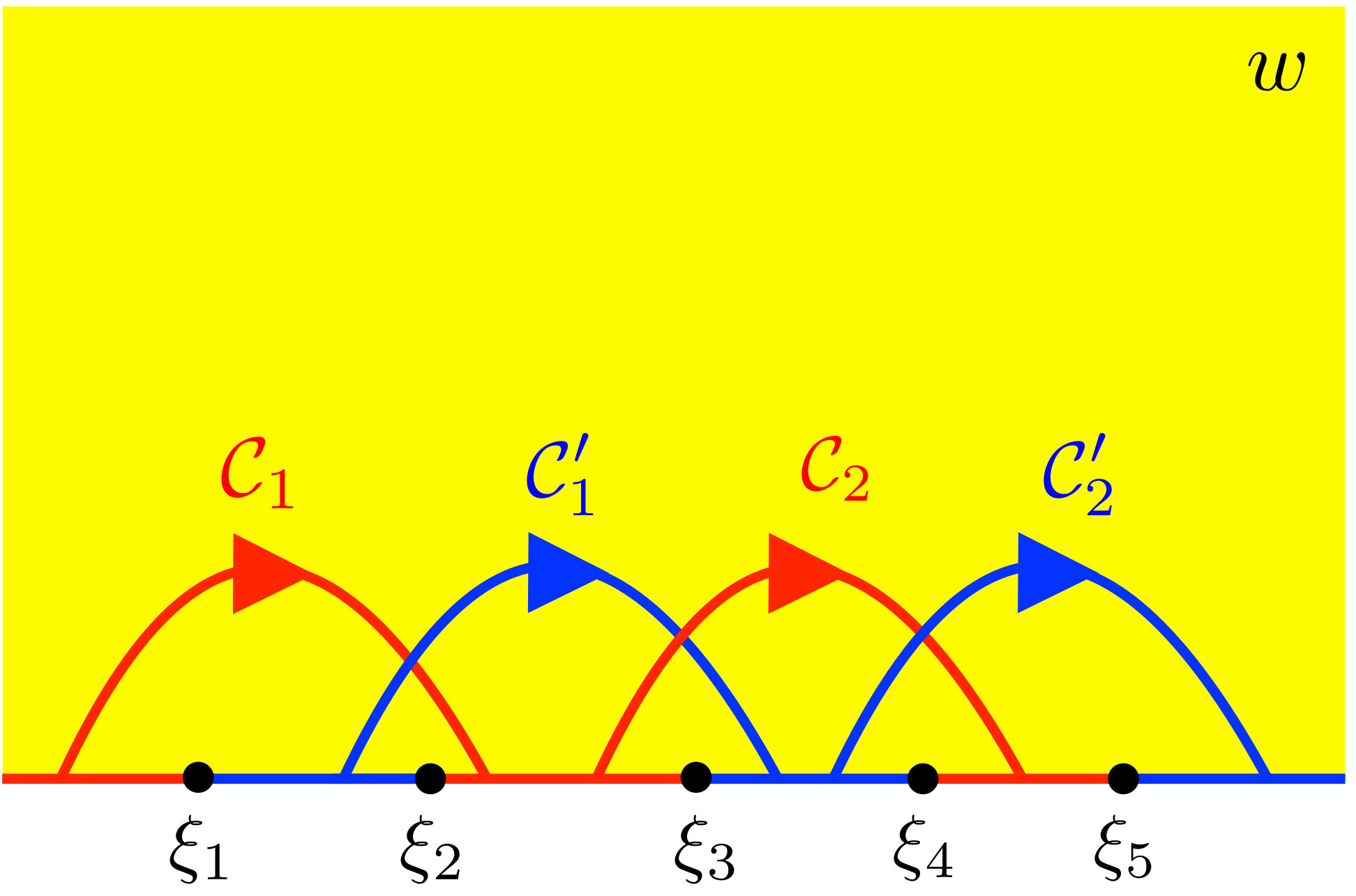 Figure 1
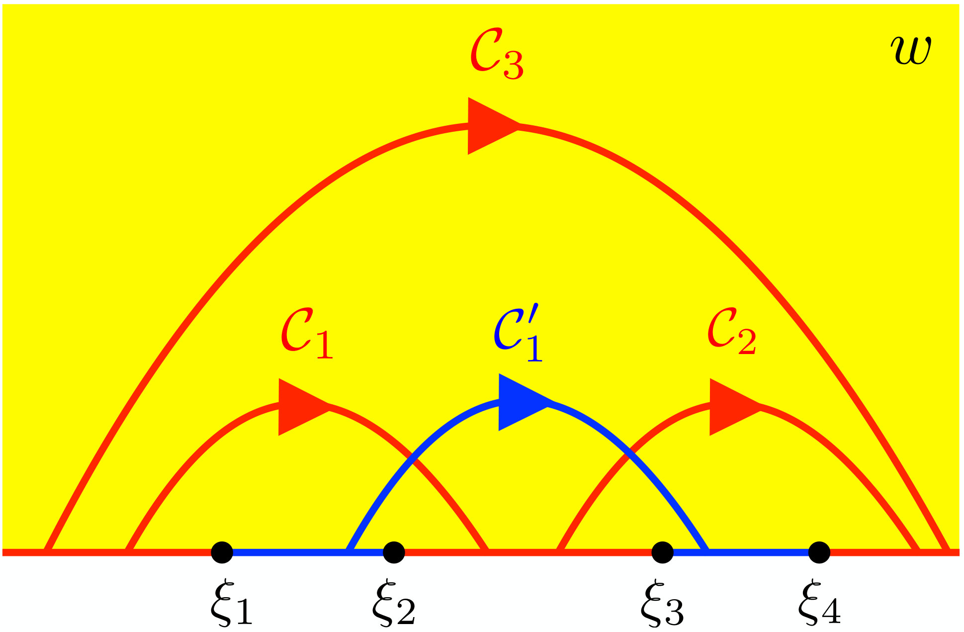 Figure 2
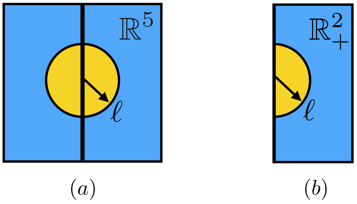 Figure 3
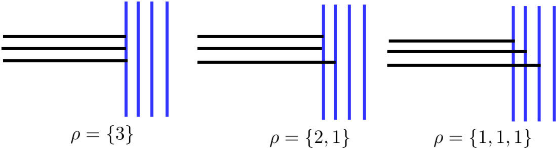 Figure 1
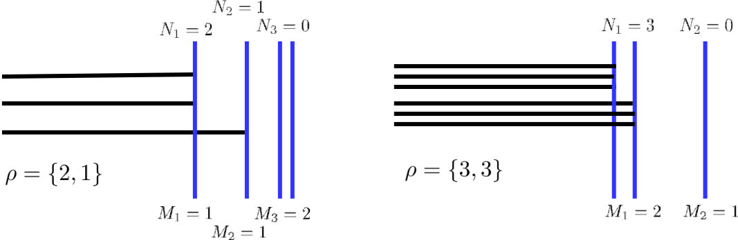 Figure 2
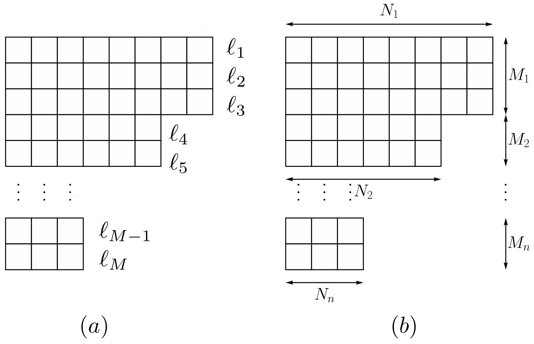 Figure 6
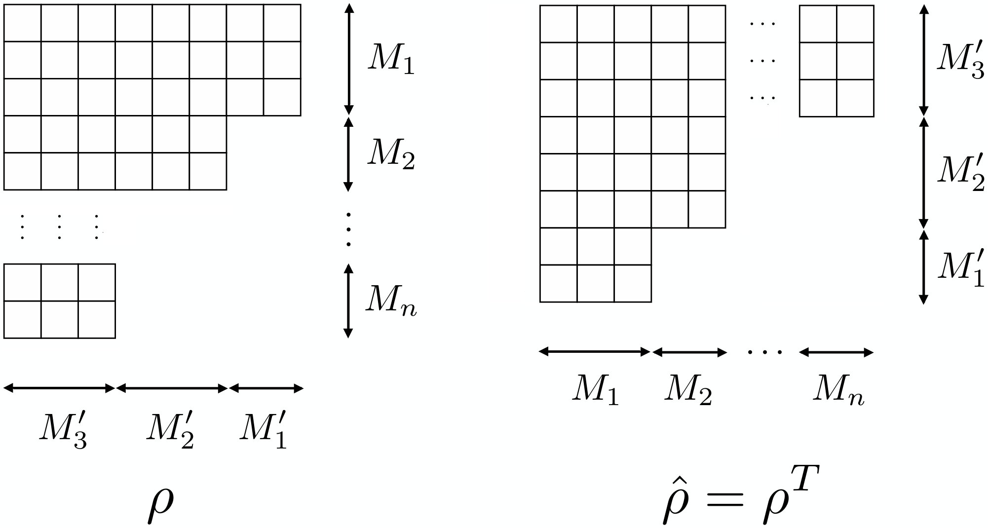 Figure 7
Peer Reviews
No public reviews on file for this paper yet. If you reviewed it on a platform where reviews are public (OpenReview, ICLR, NeurIPS, ICML), you can paste yours below so the community can read it here.
Videos
No videos yet. Explain this paper in a talk, walkthrough, or lecture? Add one.
11institutetext: New York City College of Technology, City University of New York, 300 Jay Street, Brooklyn, NY, 11201, USA22institutetext: STAG Research Centre, Physics and Astronomy, University of Southampton, Highfield, Southampton SO17 1BJ, UK
Wilson Surface Central Charge from Holographic Entanglement Entropy
John Estes 1
Darya Krym 2
Andy O’Bannon 2
Brandon Robinson 2
and Ronnie Rodgers
Abstract
We use entanglement entropy to define a central charge associated to a two-dimensional defect or boundary in a conformal field theory (CFT). We present holographic calculations of this central charge for several maximally supersymmetric CFTs dual to eleven-dimensional supergravity in Anti-de Sitter space, namely the M5-brane theory with a Wilson surface defect and three-dimensional CFTs related to the M2-brane theory with a boundary. Our results for the central charge depend on a partition of M2-branes ending on M5-branes. For the Wilson surface, the partition specifies a representation of the gauge algebra, and we write our result for the central charge in a compact form in terms of the algebra’s Weyl vector and the representation’s highest weight vector. We explore how the central charge scales with and for some examples of partitions. In general the central charge does not scale as or , the number of degrees of freedom of the M5- or M2-brane theory at large or , respectively.
Keywords:
AdS/CFT correspondence, Gauge/gravity correspondence
1 Introduction
M-theory is currently the leading candidate for an ultra-violet (UV) complete theory of quantum gravity. M-theory is defined as the (presumably unique) UV completion of 11d supergravity (SUGRA), which is a remarkably simple theory Becker:2007zj ; West:2012vka : the only bosonic fields are the metric and a three-form, . The stable BPS solitons of 11d SUGRA include M2- and M5-branes charged under electrically and magnetically, respectively. A complete formulation of M-theory will necessarily entail understanding these M-branes and other non-perturbative objects of 11d SUGRA more fully.
In a fashion similar to strings ending on D-branes or D-branes ending on other D-branes Strominger:1995ac , M2-branes can end on M2- or M5-branes, and M5-branes can end on other M5-branes. When the distance between two parallel D-branes shrinks to zero, the strings stretched between them become massless point particles and give rise to non-Abelian gauge multiplets. The low-energy worldvolume theory of multiple coincident D-branes is thus a maximally supersymmetric (SUSY) non-Abelian gauge theory Witten:1995im . However, when parallel M2- or M5-branes become coincident, the M2- or M5-branes stretched between them that become massless are extended objects, not point particles—making the low-energy worldvolume theory more challenging to identify.
For M2-branes the low-energy theory turns out to be a conventional quantum field theory (QFT), and in fact a conformal field theory (CFT): the low-energy theory of coincident M2-branes at a singularity is a 3d SUSY Chern-Simons-matter theory, called the Aharony-Bergman-Jafferis-Maldacena (ABJM) theory Bagger:2006sk ; Gustavsson:2007vu ; Bagger:2007jr ; Bagger:2007vi ; Aharony:2008ug . When the Chern-Simons level or the SUSY is enhanced to . When ABJM is holographically dual to 11d SUGRA on Maldacena:1997re . The CFT and holographic descriptions have provided a wealth of information about M2-branes. For example, at large the number of worldvolume degrees of freedom scales as Klebanov:1996un ; Drukker:2010nc .
For coincident M5-branes the low-energy worldvolume theory is less well-understood. The 11d SUGRA soliton solution for M5-branes indicates that the worldvolume theory has 6d SUSY and that the worldvolume fields should consist of five scalars, a chiral two-form , and their fermionic superpartners filling out a tensor multiplet Kaplan:1995cp . The fields in the tensor multiplet arise as Goldstone modes: the scalars from breaking translations in the five normal directions, from breaking the symmetry of shifting by the exterior derivative of a two-form, and the fermions from breaking half the SUSY. The SUSY has R-symmetry, which acts to rotate the five transverse directions, hence the five scalars transform as a vector of . The existence of the chiral in the tensor multiplet means that the three-form field strength, , is self-dual on the M5-brane worldvolume, i.e. . Furthermore the tensor multiplet fields are believed to be valued in a worldvolume gauge algebra Strominger:1995ac . We will henceforth ignore the overall representing the center-of-mass motion of the coincident M5-branes.
The existence of is also intuitive because an M2-brane ending on an M5-brane produces in the M5-brane worldvolume a 2d 1/2-BPS soliton, i.e. a string, which naturally couples to Howe:1997ue . Moreover, implies that this string has equal electric and magnetic charges, and hence is called a “self-dual string.” When the distance between two parallel M5-branes goes to zero and hence the M2-branes stretched between them become massless, the result should be a 6d theory of massless self-dual strings Strominger:1995ac .
Since strings are extended objects, such a perspective suggests that the M5-brane theory might be non-local. However, compelling evidence has accumulated that in fact the M5-brane theory is not only local, but is a conventional CFT. In particular, when the 11d SUGRA soliton solution for M5-branes has a near-horizon geometry in the decoupling limit, suggesting that 11d SUGRA on should be holographically dual to the M5-brane theory Maldacena:1997re . The factor indicates that all 6d field theory observables computed holographically are consistent with those of a local CFT. Additionally, non-trivial solutions to 6d conformal bootstrap equations have been found that are consistent with SUSY and locality Beem:2015aoa .
From the perspective of conventional, perturbative QFT, the existence of any unitary, interacting QFT in is surprising, since power counting rules out any local Lagrangian. Two additional challenges arise in writing a local Lagrangian for the M5-brane theory. First, imposing self-duality at the level of the Lagrangian in any dimension is difficult. Second, generalizing gauge transformations to a higher-form gauge field, such as the two-form , is challenging. Remarkably, for the Abelian case, , a classical action for the M5-brane worldvolume fields that has gauge invariance, superconformal symmetry, and locality, as well as 6d self-duality of enforced by auxiliary scalar field (acting as a Lagrange multiplier), is known Pasti:1997gx ; Bandos:1997ui . However, whether a classical action can be written for remains unknown.
Despite the challenges, the M5-brane theory is extremely important to study, not only because M5-branes are key ingredients of M-theory, but also because the M5-brane worldvolume theory holds a uniquely privileged place among QFTs. In 6d, is the maximal amount of SUSY possible, and 6d is the maximal dimension in which superconformal symmetry is possible Nahm:1977tg . A 6d SUSY CFT cannot be reached as the infra-red (IR) fixed point of a local renormalization group (RG) flow from a free UV fixed point. The M5-brane theory has no known dimensionless parameters besides that could be tuned to allow a perturbative expansion. In short, the dimensionality, symmetries, and determine the M5-brane theory completely. The M5-brane theory is thus an isolated, intrinsically strongly-interacting fixed point. Via compactification the M5-brane theory can describe many lower-dimensional SUSY QFTs and dualities among them, and could potentially be a “master theory” containing information about all lower-dimensional QFTs.
In this paper, we will use holography to study the M5-brane theory with a 2d conformal defect as well as 3d CFTs with boundaries (BCFTs) related to the ABJM BCFT, using the following 1/4-BPS intersection of M-branes:
[TABLE]
Schematically, this table represents a stack of coincident M2-branes, a stack of coincident M5-branes, and another stack of coincident M5-branes that we label M5*′* to distinguish them from the first stack. Most importantly, the M2-branes end on the M5- and M5*′*-branes at .
Consider first setting , that is, the intersection of M2-branes ending on M5-branes, with no M5*′*-branes. Recall that the endpoint of a semi-infinite string ending on a D-brane gives rise to an infinitely massive (s)quark in the D-brane’s worldvolume. Integrating out the heavy (s)quark yields a Wilson line, i.e. the holonomy of the D-brane worldvolume gauge field along the (s)quark worldline Maldacena:1998im ; Rey:1998ik . Similarly, the end of a semi-infinite M2-brane ending on an M5-brane produces a self-dual string with infinite tension, which can be integrated out to yield a “Wilson surface” operator Ganor:1996nf . In the Abelian case, , a precise form is known for the 1/2-BPS Wilson surface operator, , with the integral over the surface spanned by the self-dual string and the ellipsis denoting terms required by SUSY, involving the M5-branes’ worldvolume scalars, see for example ref. Bullimore:2014upa . In the non-Abelian case, , a precise form is unknown but is believed to be schematically , with the trace in representation of . The representation describes how the M2-branes are partitioned among the M5-branes, as we discuss in detail below.
We will consider only flat Wilson surfaces, i.e. Wilson surfaces extended along the spanned by and . From the M5-brane theory’s perspective the Wilson surface is a 1/2-BPS 2d superconformal soliton. The M5-brane theory’s bosonic symmetry is , where is the 6d conformal group. The table above shows that the Wilson surface preserves an subgroup, where the global 2d conformal group leaves invariant the Wilson surface, and the first rotates while the second rotates . The R subscripts indicate that these act as R-symmetries on the supercharges preserved by the Wilson surface, forming a 2d “large” SUSY (“small” has a single ).
We will compute a central charge associated with the Wilson surface using holography. The holographic description’s geometry is an and two ’s fibered over a Riemann surface D'Hoker:2008wc ; DHoker:2008rje ; Estes:2012vm ; Bachas:2013vza and hence has the expected isometry . The holographic description represents a large limit with arbitrary . The geometry is asymptotically locally for all , and becomes precisely when .
As is well-known, 2d large super-groups actually come in a one-parameter family called , where is the free parameter Sevrin:1988ew ; Frappat:1996pb . The most general solutions of 11d SUGRA that have super-isometry and locally asymptote to are known Bachas:2013vza . The bosonic subgroup of is , and hence these solutions all involve an and two ’s fibered over a Riemann surface DHoker:2008wvd . The solutions describing Wilson surfaces in the M5-brane theory at large and arbitrary have .
Additionally, the most general solutions of 11d SUGRA with super-isometry are known that locally asymptote to “half” of , in a sense we explain below Bachas:2013vza . These solutions are holographically dual to 3d maximally SUSY BCFTs. The exact BCFTs are not yet known, though some properties are clear from the 11d SUGRA solutions. In particular, in these solutions generically both and are non-zero. The solutions thus describe M2-branes ending on M5- and M5*′*-branes, and hence the BCFTs must be cousins of the maximally SUSY ABJM BCFT.111Solutions of 11d SUGRA that are candidates for the holographic dual of the maximally SUSY ABJM BCFT appear in ref. Bachas:2013vza , but have potentially dangerous singularities. Presumably these BCFTs are obtained from the ABJM BCFT by couplings to 2d SUSY multiplets at the boundary, and/or by sources or expectation values of scalar operators away from the boundary, similar to the superconformal interfaces between ABJM theories in refs. DHoker:2009lky ; Bobev:2013yra . We will henceforth refer to these theories as “cousins of the ABJM BCFT.”
For or , ABJM’s bosonic symmetry is enhanced to , where is the 3d conformal group, and in the intersection above the acts on . Maximally superconformal boundary conditions at preserve the that leaves the boundary invariant, and R-symmetry. The maximally SUSY ABJM BCFT’s bosonic symmetry is thus , and the super-group of the theory is with . The cousins of the maximally SUSY ABJM BCFT that we will study have arbitrary , and their holographic duals again involve an and two ’s fibered over a Riemann surface Bachas:2013vza . These solutions correspond to a limit with large and a large number of M5- and M5*′-branes. However the values of and are in fact undetermined, intuitively because the M2-branes do not “know” how many M5- and M5′-branes have zero M2-branes ending on them, and so cannot know the total numbers of M5- and M5′*-branes. Additionally, sending both and to zero produces a singular solution, presumably because removing a BCFT’s boundary is a singular operation.
Using these 11d SUGRA solutions, we will compute a central charge associated with the Wilson surface or 3d BCFT boundary. Crucially, the Wilson surface or 2d boundary is not a 2d CFT, but a 2d defect in, or boundary of, an ambient CFT that has , which implies in general that the full Virasoro symmetry is not present. To be more precise, the Wilson surface or boundary breaks the ambient or conformal symmetry down to , i.e. the global part of the Virasoro symmetry, in which the usual central charge does not appear. We must therefore define a central charge some other way.
We will use entanglement entropy (EE). Following refs. Jensen:2013lxa ; Estes:2014hka ; Gentle:2015jma , we will compute holographically the EE of a spherical region centered on the 2d defect or of a semi-circle centered on the 2d boundary. This EE has UV divergences, as expected, so we introduce a UV cutoff and subtract the EE of the ambient CFT. What remains is a term logarithmic in the cutoff, a constant term, and terms that vanish as the cutoff is removed. In analogy with the EE of a single interval in a 2d CFT Holzhey:1994we ; Calabrese:2004eu , we identify the coefficient of that logarithmic term as times the central charge. In short, we compute the change in the coefficient of the EE’s logarithmic term due to the 2d defect or boundary, and use the result to define a central charge. We will denote the resulting Wilson surface or 2d boundary central charge as or , respectively. Again in analogy with 2d CFT, we will interpret these as counting massless degrees of freedom supported on the Wilson surface or 2d boundary.222In a 3d BCFT the boundary central charge defined from EE is proportional to a central charge that appears in the trace anomaly Fursaev:2013mxa ; Fursaev:2016inw and obeys a c-theorem, strictly decreasing in a boundary RG flow Jensen:2015swa . Our thus counts massless degrees of freedom at the 2d boundary. However, a similar interpretation of may not always be justified. In particular, examples of defects in higher-d CFTs are known in which central charges defined from EE do not decrease along defect RG flows Kumar:2016jxy ; Kumar:2017vjv ; Kobayashi:2018lil . These examples include certain RG flows on a Wilson surface in a totally symmetric representation Rodgers:2018mvq . Whether and how these central charges defined from EE are related to other potential definitions, for example via the thermodynamic entropy, stress tensor correlators, and so on, we leave as an important open question.
Our main result, for , takes a remarkably simple form,
[TABLE]
where is the highest weight vector of the Wilson surface’s representation , is the Weyl vector, and is defined with the Killing form on the weight space. The inner product is invariant under the action of the Weyl group, hence so is . In particular, is invariant under complex conjugation of a representation, , which acts as a Weyl reflection. Eq. (1.1) is also reminiscent of the results for the M5-brane theory’s own central charges, and , which can similarly be written in terms of purely group theoretic data Beem:2014kka ; Cordova:2015vwa . However, eq. (1.1) obscures ’s dependence on and . In sec. 4 we present for some specific , such as the rank totally symmetric and anti-symmetric representations, to explore the dependence on and . Our results for cannot be written so neatly as eq. (1.1), largely because we do not know the total number of M5- and M5*′*-branes and thus do not know or .
However, a key observation about our results for both and is that neither naturally scales as , characteristic of M2-branes at large Klebanov:1996un ; Drukker:2010nc , or as , characteristic of M5-branes at large ( at large ) Freed:1998tg ; Harvey:1998bx ; Henningson:1998gx . In other words, in general for the M-brane intersections we consider, the number of massless degrees of freedom on the Wilson surface or 2d boundary does not scale, in any obvious way, with the total number of degrees of freedom of the M2- or M5-brane theory.
This paper is organized as follows. In sec. 2 we review the 11d SUGRA solutions describing M5-branes with Wilson surfaces or cousins of the ABJM BCFT with . In sec. 3 we derive an integral for the holographic EE, and then evaluate the integral to extract and . In sec. 4 we summarize our results, including for specific , and compare to existing results. (Readers interested only in our results can skip directly to sec. 4.) We conclude in sec 5 with discussion and suggestions for future research.
The companion paper ref. Rodgers:2018mvq reproduces our results for for the fundamental, totally anti-symmetric, and totally symmetric representations, using probe branes in , namely a probe M2-brane when or M5-brane when . Ref. Rodgers:2018mvq also uses the probe M5-branes to explore RG flows on Wilson surfaces.
Note added: After this paper appeared on the arxiv, ref. Jensen:2018rxu clarified how our central charge obtained from the EE of a (hemi-)sphere is related to central charges in the defect’s contribution to the Weyl anomaly. This clarifies the relationship between unitarity and positivity of discussed in sec. 4.1, among other things.
For a CFT in with and a 2d conformal defect, the trace of the stress tensor splits into two terms, , where is the CFT’s trace anomaly, which is [math] for odd but may be non-zero for even , is a delta function that localizes to the 2d defect, and Graham:1999pm ; Henningson:1999xi ; Schwimmer:2008yh
[TABLE]
where is the defect’s induced metric (), is the Ricci scalar built from , is the defect’s traceless extrinsic curvature, is the Weyl tensor pulled back to the defect, and the dimensionless numbers , , and are the defect central charges. In a 3d BCFT the boundary’s contribution to the trace anomaly has the form of eq. (1.2), but identically, so does not exist. All of , , and can depend on boundary conditions imposed on CFT fields at the defect or boundary and on degrees of freedom supported only at the defect or boundary. Indeed, obeys a -theorem Jensen:2015swa , and may thus serve as a measure of the number of massless degrees of freedom at the defect or boundary. However, unlike a 2d CFT’s central charge, unitarity does not require , and in fact even simple, unitary theories can have , such as a 3d free, massless scalar BCFT with Dirichlet boundary conditions Nozaki:2012qd ; Jensen:2015swa ; Solodukhin:2015eca . Whether a lower bound exists on remains unknown, though for 3d BCFTs is conjectured Herzog:2017kkj , where unitarity requires Herzog:2017xha ; Herzog:2017kkj . Ref. Jensen:2018rxu showed that if the average null energy condition is valid in a CFT with a 2d conformal defect, then also.
Refs. Kobayashi:2018lil ; Jensen:2018rxu showed that
[TABLE]
For , as is the case for the cousins of ABJM, this reproduces the result Fursaev:2013mxa ; Fursaev:2016inw . For , eq. (1.3) implies that may be negative even when and are both positive. Indeed, for Wilson surfaces in the M5-brane theory, ref. Jensen:2018rxu used eq. (1.3), our result for in eq. (1.1), and the result of ref. Gentle:2015jma for to calculate
[TABLE]
both of which are positive for any . However, the linear combination in eq. (1.3) can be negative for some , as we discuss in sec. 4.1. These results show that does not signal violation of unitarity.
2 Review: the SUGRA Solutions
The solutions of 11d SUGRA in ref. Bachas:2013vza that holographically describe Wilson surfaces or cousins of the ABJM BCFT (and which built upon the solutions in refs. DHoker:2008rje ; D'Hoker:2008wc ; Estes:2012vm ) are 1/2-BPS, meaning they support 16 real supercharges, and have super-isometry with . The super-group has bosonic subgroup , where the super-charges anti-commute into a linear combination of the generators of these three bosonic factors. The parameter determines the relative weights of the coefficients in that linear combination. The super-group is invariant under the simultaneous operations and swapping the two ’s. Without loss of generality we can thus restrict to , and in fact all the solutions we consider below will have . These symmetries of the 11d SUGRA solutions match those of 2d large SUSY, which admits exactly the same one-parameter family of Lie super-groups Sevrin:1988ew ; Frappat:1996pb .333Ref. Sevrin:1988ew classifies and constructs the Virasoro extension of the super-group. We leave the full details of these 11d SUGRA solutions to refs. Bachas:2013vza ; DHoker:2008rje ; D'Hoker:2008wc ; Estes:2012vm , and here review only features that we will need in subsequent sections. In particular, we will consider the solutions of refs. DHoker:2008rje ; Bachas:2013vza , using the conventions of ref. Bachas:2013vza .444To clarify, ref. D'Hoker:2008wc constructed solutions for three special values of , ref. Estes:2012vm constructed the solutions for general , and refs. DHoker:2008rje ; Bachas:2013vza identified the specific solutions we consider in this paper.
The isometry implies that the metric involves and two ’s fibered over a Riemann surface, which we take to be the upper half plane,
[TABLE]
where and are the coordinates of the upper half plane (so ). The functions , , , and depend only on and . We denote by the metric for a unit-radius round and the metric for a unit-radius , that is,
[TABLE]
where , with boundary at , is the time coordinate, and is the spatial coordinate parallel to the Wilson surface or 2d boundary.
The solutions in ref. Bachas:2013vza that we will use are completely determined by a triple of data , where is a harmonic function over the upper half plane, and is a complex-valued function that obeys
[TABLE]
although is not completely determined by . If we define the complex-valued functions
[TABLE]
where is the constant parametrizing the supergroup, then in these solutions , , , and are given by
[TABLE]
The parameters , , and are constants that obey , so that only two are independent. In fact, a simultaneous re-scaling of , , and can be absorbed by re-scaling without changing the solution, so only a single constant is independent. That single constant must map to : the precise relation is . As mentioned above, the solutions that we will consider have .
When , global regularity of these solutions requires that and obey and everywhere on the interior of the upper half plane (all ) and that and on the boundary of the upper half plane (). All the solutions that we consider below will obey these conditions.
The four-form of these solutions appears in ref. Bachas:2013vza . We will not present the solution for explicitly, but in sec. 2.3 we will discuss the M2- and M5-brane charges determined by the solution for .
The invariance of under and swapping of sub-groups appears in these 11d SUGRA solutions as invariance under and exchange of . As clear from eq. (2.9), that leaves and invariant but trades , thus effectively interchanging the geometry’s two factors.
2.1 Asymptotically Locally Solutions
The 11d SUGRA solutions holographically describing Wilson surfaces in the M5-brane theory at large are of the form in eq. (2.5) with
[TABLE]
where the integer and the are real-valued constants determining ’s branch points on the boundary of the upper half plane. More specifically, the are points on the real line where changes sign from to .
In general, the upper half plane is invariant under the group of transformations, which is three-dimensional. Implicitly we fixed two transformations with our choice of . The third transformation is translations, which we can use to fix one of the . The remaining values of the determine the M2- and M5-brane charges of the solution, as we discuss in sec. 2.3. The solutions describing M2-branes ending on M5-branes have , whereas describes M2-branes ending on M5*′*-branes. However the latter map to the former via and swapping the two ’s, as described above. In what follows, we will consider arbitrary in many intermediate steps but will always set in our final results.
Another form of the in eq. (2.10) that will be useful for describing the geometry’s asymptotics comes from using polar coordinates in the upper half plane, with and . If we expand in Legendre polynomials, ,
[TABLE]
then the determine the expansion coefficients , where is finite but .
Though not immediately obvious, the solutions in eq. (2.10) are asymptotically locally . Indeed, asymptotically we can put the metric of these solutions in the Fefferman-Graham (FG) form of ,
[TABLE]
where is the FG holographic coordinate, with boundary at , is the distance to the defect, is the zenith angle of the asymptotic , and the ellipsis represents terms sub-leading in . The change of coordinates to FG form admits the following asymptotic expansion,
[TABLE]
which determines the radius of curvature of the asymptotic ,
[TABLE]
The factor in eq. (2.12) indicates that for generic the dual M5-brane theory lives on a space with a conical singularity at . These 11d SUGRA solutions thus suggest that deformations of the M5-brane theory with super-group are only possible, for generic , on spaces with such a conical singularity. Only for does the singularity disappear such that the theory lives on 6d Minkowski space.
Eqs. (2.12) and (2.13) show clearly that in these solutions we can approach the asymptotic boundary in two ways. First, if we fix and send then with fixed , which means that we arrive at the boundary a distance from the defect. Second, if we fix and send , then but now , and so we arrive at the boundary precisely on the defect. Recall from eq. (2.6) that is the boundary of the factor.
The solution is simply the and case, which has two branch points. Using the translational symmetry we place these two branch points on the real line symmetrically, at , such that the solution has only one free parameter, . In this case, in eq. (2.13) the higher-order powers of vanish, and hence the ellipsis in eq. (2.12) vanishes. We will see below that determines and hence , the single free parameter of the solution. The cases with and then describe Wilson surfaces in the M5-brane theory.
2.2 Asymptotically Locally Solutions
The 11d SUGRA solutions holographically describing cousins of the ABJM BCFT with are of the form in eq. (2.5) with
[TABLE]
where the integer and the are real-valued constants determining ’s branch points on the boundary of the upper half plane, i.e. on the real line . As in sec. 2.1, we have implicitly fixed two transformations of the upper half plane with our choice of , and we can use translation symmetry to fix one of the . The remaining values of the then determine the solutions’ M2- and M5-brane charges, as we discuss in sec. 2.3. We will consider solutions with .
As in sec. 2.1, we can obtain another form of the in eq. (2.15) that will be useful for describing the asymptotics by introducing with and . Expanding in Legendre polynomials then gives
[TABLE]
where the determine the expansion coefficients .555We use the same symbol for the expansion coefficients in both eq. (2.11) and (2.16), though the difference should always be clear from the context.
The solutions in eq. (2.10) are in fact asymptotically locally “half” of , in the following sense. Asymptotically we can put the metric of these solutions in the FG form of ,
[TABLE]
where the ellipsis represents terms sub-leading in , and where the asymptotic radius, , is given by
[TABLE]
The change of coordinates to FG form has the following asymptotic expansion,
[TABLE]
where implies . Eq. (2.19) shows that implies the FG holographic coordinate , with boundary at , but crucially . The background geometry for the holographically dual field theory thus has coordinates , , and , i.e. half of 3d Minkowski space with a boundary at . In this sense, these solutions are locally asymptotic to “half” of , as advertised.
As a result, no continuous limit exists in which these solutions reduce to the exact solution. In fact, the exact solution differs from these solutions in several ways. For example, in these solutions the in eq. (2.15) has a single pole at , and , whereas in the exact solution has two poles and . Since we cannot continuously send , the BCFTs holographically dual to our solutions therefore appear to be cousins of, but not continuously connected to, the ABJM BCFT. Identifying the dual BCFTs is an important question we leave for future research.
Eqs. (2.17) and (2.19) also show that, as in sec. 2.1, we can approach the asymptotic (half) boundary in two ways. First, if we fix and send , then with fixed , so that we arrive at the boundary a distance from the BCFT’s boundary. Second, if we fix and send , then but now , and so we arrive at the boundary precisely on the BCFT’s 2d boundary.
2.3 Partitions and M-brane Charges
The M-brane intersection of sec. 1 describes coincident M2-branes ending on coincident M5-branes and coincident M5*′-branes. Such an intersection is characterized by a partition of describing which M5- or M5′*-brane each M2-brane ends on. In this section we will briefly sketch how we extract this partition from the 11d SUGRA solutions reviewed above, leaving the full details to ref. Bachas:2013vza .
The asymptotically locally solutions of sec. 2.1 describe M2-branes ending only on M5-branes, not on M5’-branes, and are fully characterized by a partition of M2-branes among the M5-branes. The asymptotically locally solutions of sec. 2.2 describe M2-branes ending on both M5 and M5’-branes, but are still fully characterized by a partition of M2-branes among M5-branes. The special features of both solutions will be discussed in more detail below. Our discussion of the partitions will applies to both solutions, with one crucial exception: the partitions of the solutions include cases in which some M5-branes have no M2-branes ending on them, whereas the solutions do not admit such partitions.
We will denote the partition as , which we will order with entries decreasing from left to right. To illustrate which M2-brane ends on which M5-brane, we will temporarily imagine separating the M2-branes in one of the directions and separating the M5-branes in the direction, as shown in figs. 1 and 2. Once is specified we will re-collapse the M2- and M5-branes back to the original intersection of coincident stacks.
We will use two parametrizations of . In the first parametrization we label as the number of M2-branes ending on the M5-brane and write the partition as with integers . In this parametrization the total number of M5-branes is simply the upper limit of , while the total number of M2-branes is
[TABLE]
We allow for some , representing M5-branes with zero M2-branes ending on them. However, when writing we will omit all zero entries. As examples, fig. 1 shows all for the case with and .
In the second parametrization we write the partition as
[TABLE]
representing M5-branes each with M2-branes ending on them, M5-branes each with M2-branes ending on them, and so on with . In other words, the are distinct non-zero integers, each with degeneracy . The final entries in are , with degeneracy , representing the number of M5-branes with no M2-branes ending on them. We thus specify by specifying the set of integers and the set of their degeneracies . The partition has a total of parameters, the distinct integers in plus the distinct integers in . In this parametrization the total numbers of M2-branes and of M5-branes are
[TABLE]
As in the first parametrization, when writing we will omit all zero entries, that is, we omit the entries . As examples, fig. 2 shows the sets and for with (fig. 2 left) and with (fig. 2 right).
The ordered partition determines a Young tableau, with the physical interpretation that each box in the Young tableau represents an M2-brane and each row represents an M5-brane. In the first parametrization, with , each gives the number of boxes in the row of the Young tableau, as shown in fig. 3 (a). In the second parametrization, eq. (2.21), is the number of rows with boxes, is the number of rows with boxes, and so on, as shown in fig. 3 (b).
When the M2- and M5-branes re-collapse back to the original intersection of coincident stacks, the gauge algebra on the M5-branes’ worldvolume is and the M2-branes’ boundary represents the Wilson surface. The partition , or the corresponding Young tableau, then determines the Wilson surface’s representation of . Complex conjugation of the representation, , acts in the first parametrization as and in the second parametrization as
[TABLE]
As mentioned above, the asymptotically locally solutions are also fully characterized by a partition of . Crucially, however, the partition will have only non-zero entries, as we explain below. In particular, in the parametrization by and we will not have a value for . Eq. (2.22) will thus give us but not . Of course, generically the with will be non-zero, so we know must be non-zero, but we will not be able to fix its value. In the parametrization all the will be non-zero, and the total number will still be a sum of the as in eq. (2.20), though the upper limit of the sum will be . In a similar fashion, the asymptotically locally solutions will have whose value we will not be able to fix. Without or we will not be able to identify gauge algebras or . The partition will still specify a Young tableau, as described above, but without an algebra we will not be able to identify a representation with the Young tableau.
2.3.1 Asymptotically Locally Solutions
In the asymoptotically locally solutions reviewed in sec. 2.1, no explicit M2- or M5-brane sources appear in the 11d SUGRA equations. However, the solutions have non-zero flux of the 11d SUGRA 4- or 7-form wrapping closed, non-contractible 4- or 7-cycles, respectively. Presumably the M2- and M5-branes have been replaced by these fluxes, or “dissolved into flux,” similar to how D3-branes are replaced by five-form flux in the solution of type IIB SUGRA (i.e. how open string degrees of freedom are replaced by closed string degrees of freedom). As explained in ref. Bachas:2013vza , from these fluxes we can recover an ordered partition and hence a Wilson surface representation , as follows.
How do we identify closed, non-contractible 4- and 7-cycles in the geometry eq. (2.5) with the and of eq. (2.10)? As an example, fig. 4 shows the upper-half complex plane for , that is, with branch points on the axis, , , , . Fig. 4 also shows that geometry’s three independent non-contractible 4-cycles, the curves , , and , and a single, non-independent 4-cycle, , obeying . However, unlike the other 4-cycles, can be continuously deformed to .
To see why the curves , , and determine closed, non-contractible 4-cycles, recall from sec. 2 that the geometry has two ’s, and that regularity requires and on the axis. At each point on the axis one of the two ’s collapses to a point, while the other does not. Specifically, from eqs. (2.5), (2.8), and (2.9) we see that and implies while , and so one collapses to a point while the other does not. Conversely, and implies and interchanging the behavior of the two ’s. When we cross a branch point , flips sign from to , which implies that different ’s collapse to a point on the two sides of . As a result, any curve in the upper-half complex plane that begins on the axis, jumps over two branch points, and then ends on the axis, when combined with the that collapses at the curve’s endpoints, forms a closed, non-contractible 4-cycle. In contrast, a curve jumping over an odd number of branch points does not define a closed 4-cycle. Each closed, non-contractible 4-cycle also defines a closed, non-contractible 7-cycle: given a 4-cycle in which one collapses, simply take the product with the that does not collapse. In short, every consecutive pair of branch points defines a closed, non-contractible 4-cycle and 7-cycle.666A word of caution: in ref. Bachas:2013vza the notation refers only to a curve in the upper-half plane, while in this paper it refers to a 4-cycle, i.e. the curve times the that collapses at the curve’s endpoints. Correspondingly, in this paper a 7-cycle will be denoted .
As mentioned above, in fig. 4 the 4-cycle can be decomposed as , and can be continuously deformed to . As mentioned below eq. (2.13), fixing and sending takes us to the asymptotic boundary a distance from the defect, and so we identify the 4-cycle at as the of the asymptotic local .
The total number of non-contractible 4-cycles in these geometries is , i.e. the number of branch points minus one. The number of non-contractible cycles thus matches the number of free parameters in the solution: as mentioned in sec. 2.1, we can fix one of the branch points using translations, leaving free parameters.
Integrating over a non-contractible 4-cycle yields a charge that we interpret as a number of dissolved M5- or M5*′*-branes. We will not write the explicit form for , which appears in ref. Bachas:2013vza , but we will need the explicit forms for these charges in terms of the locations of branch points . In the upper-half complex plane and starting from the left-most cycle, let , with , denote the independent non-contractible 4-cycles all involving the same collapsing . In the example above these are the 4-cycles and . Anticipating their role in a partition , we refer to the integrals of the 4-form flux over as , i.e.
[TABLE]
with the 11d Newton’s constant. For , turns out to be proportional to (minus) the distance between two consecutive branch points Bachas:2013vza :777As mentioned below eq. (2.9), these solutions are invariant under simultaneous re-scaling of and . Re-scaling clearly means re-scaling and hence the branch points . As a result, the charges , , and in eqs. (2.25), (2.26), and (2.30), respectively, are invariant under the re-scaling.
[TABLE]
We have chosen an orientation so that for positive and , the are positive. In the upper-half complex plane and starting from the left-most cycle, let , with , denote the independent non-contractible 4-cycles that all involve the same collapsing orthogonal to the that collapses in the cycles. In the example above, this is the 4-cycle . Since the that collapses in the is orthogonal to that of the , we refer to the integral of the 4-form flux over as M5*′*-brane charge, which we denote . We define with the same conventions as eq. (2.24). For , also turns out to be proportional to the distance between two consecutive branch points Bachas:2013vza ,
[TABLE]
Again, we have chosen the orientation so that for positive and , the are positive. Such M5*′-brane charge presumably arises from brane polarization, a.k.a. the Myers effect Myers:1999ps : the M2-branes source in a background with non-zero from the M5-branes, so that the Wess-Zumino (WZ) term in the 11d SUGRA action produces non-trivial flux orthogonal to that of the M5-branes, i.e. M5′-brane flux.888The presence of M5′-branes is also related to the fact that totally anti-symmetric representations can be described by a probe M5′*-brane in , wrapping and Lunin:2007ab .
The 4-cycle at identified as the in the asymptotically locally region can be decomposed as . Correspondingly, the 4-form flux through that cycle determines the total number of M5-branes, . Using eq. (2.25), we can relate to the coefficient defined in the Legendre polynomial expansion of eq. (2.11),
[TABLE]
Plugging eq. (2.27) into eq. (2.14) we thus recover the usual relation between and the radius of the asymptotic ,
[TABLE]
In contrast to the 4-form flux, the integrated 7-form flux, which we interpret as the number of dissolved M2-branes, is ambiguous: due to the WZ term in the 11d SUGRA action, when we cannot define 7-form flux that is simultaneously local, conserved, quantized, and invariant under large gauge transformations of Marolf:2000cb . At best we can define 7-form flux that has three of these properties but not the fourth. Following ref. Bachas:2013vza we will use the 7-form flux that gives the Page charge, which is local, conserved, and quantized, but not gauge invariant. Explicitly, we will integrate over a closed, non-contractible 7-cycle, where the term comes from the WZ term, and clearly produces a M2-brane charge that is not invariant under large gauge transformations of .
With that choice, to extract a fixed value of M2-brane charge we must fix a gauge of , which we do as follows. In the solutions of ref. Bachas:2013vza , can be written as a sum of three terms, one with legs along , and two with legs along the two ’s, respectively. Let denote the term with legs along the that collapses in a 4-cycle but not in a 4-cycle . To gauge-fix, we demand that when the collapses at one endpoint of one of the .999Regularity demands that vanish whenever it wraps a vanishing cycle, so our gauge choice simply enforces regularity. However, due to the presence of M5-branes we can make well defined only on a patch. The entire geometry can be covered with patches corresponding to gauge choices. Since the geometry has 4-cycles , each with two endpoints, we have choices of such endpoints, namely the left end-point of each 4-cycle plus the right endpoint of the right-most 4-cycle. For any such choice, in the solutions of ref. Bachas:2013vza the M2-brane charges are ordered from smallest to largest as we move from left to right in the upper-half complex plane, but generically include negative values. Of the gauge choices for , only one allows for the M2-brane charges to be all positive: choosing at the right endpoint of produces all positive M2-brane charges, with the right-most M2-brane charge vanishing. To see why, deform all the to lie along the real axis and note that vanishes along the real axis since it wraps a vanishing 7-cycle. The only contribution then comes from the WZ contribution . Since we have set along the cycle , the WZ contribution also vanishes along this cycle.
With gauge-fixed, and anticipating their role in a partition , we denote the integrals of 7-form flux through as , which we interpret as the total number of M2-branes ending on the M5-branes associated with ,101010Our in eq. (2.29) was defined as in ref. Bachas:2013vza .
[TABLE]
For the solutions in ref. Bachas:2013vza , and using eq. (2.26), turns out to be the sum of M5*′*-brane fluxes on all 4-cycles from to ,
[TABLE]
and where the vanishing of the right-most 7-form flux implies .
Validity of the SUGRA approximation requires curvatures to be small compared to the Planck scale. This requires the branch points to be far apart for all , and therefore for all , and also (recall the are ordered). However, with asymptotics, when the are of order unity the system should be well-described by probe branes. Taking the probe limit in our results for indeed reproduces calculations using probe branes, so our results seem to apply over a wider regime than might be expected. Similar statements about the range of validity of our results apply to what follows (i.e. the in eq. (2.35)).
The total number of dissolved M2-branes is the sum of 7-form fluxes of all the , . Eq. (2.30) shows that the 7-form fluxes through the non-contractible 7-cycles is fixed by 4-form fluxes, and hence are not independent parameters. The total number of free parameters thus remains , though we have a choice to package some of them as either the or the . In what follows we will choose the latter.
In short, eqs. (2.25) and (2.30) allow us to extract the free parameters of a partition , namely the sets of distinct non-zero integers and the distinct degeneracies , from the free parameters, i.e. the branch points , of the asymptotically locally solutions. We therefore identify the same partition determining the brane intersection, the 11d SUGRA solution, and the Wilson surface’s representation .
For a Wilson line in Yang-Mills theory all observables are invariant under the combined operations of complex conjugation of the representation, , and orientation reversal of the Wilson line. We expect the same to be true for a Wilson surface in the M5-brane theory. Indeed, we can demonstrate that these combined operations can be realized in these 11d SUGRA solutions by the combined operations of a gauge transformation of , which produces all negative M2-brane charges, followed by an orientation reversal of the 7-cycles, which flips the M2-brane charges back to being positive.
To implement these combined operations in the geometry, we start with a geometry parametrized by a partition corresponding to a representation . We perform the unique gauge transformation of that makes all the M2-brane charges negative, namely requiring at the left endpoint of . Under this gauge transformation, the are all shifted as . The shifted are thus all negative, and of course the shifted vanishes. To obtain positive M2-brane charges we reverse the orientation of the 7-cycles, thereby flipping the signs of the shifted . We can do so for example by reversing the orientation of the two ’s and the direction of integration in the upper-half plane (reversing the arrows in fig. 4). Finally, it is convenient, but not necessary, to make the coordinate transformation . This yields a geometry parametrized by a set of branch points in the same gauge we defined above eq. (2.30). Computing the M5- and M2-brane charges via eqs. (2.25) and (2.30), respectively, then reveals that the charges have been shifted as and . From eq. (2.23) we recognize this shift as complex conjugation of the representation, .
Crucially, the geometry is invariant under these combined operations. As we review in sec. 3, the CFT’s EE is proportional to the area of a minimal surface in the dual geometry Ryu:2006bv ; Ryu:2006ef ; Nishioka:2009un (eq. (3.36) below). That surface only “knows” about the geometry, and hence is invariant under any operations that leave the geometry invariant. Indeed, our results for EE, and in particular , are invariant under , as mentioned below eq. (1.1).
The operations leading to complex conjugation in these 11d SUGRA solutions have a simple interpretation in the corresponding brane intersection, as Hanany-Witten moves Hanany:1996ie . As a simple example, consider a brane intersection of the type in figs. 1 and 2, with M2-branes ending on distinct M5-branes (out of the total number of M5-branes), producing a totally anti-symmetric representation of rank . Imagine we move an M5*′-brane from infinity on the left to a finite value of , to the left of the M5-branes. If we send this M5′-brane to infinity on the right, then when the M5′-brane passes through the stack of M5-branes the M2-branes will be destroyed and anti-M2-branes will be created between the M5′-brane and each M5-brane that did not have an M2-brane ending on it. An orientation reversal then maps the anti-M2-branes to M2-branes, while the M5- and M5′*-branes are not mapped to anti-branes. Clearly the total number of M2-branes is ambiguous, as in the 11d SUGRA solutions above. Moreover, such a Hanany-Witten move clearly corresponds to complex conjugation of the representation, which for a totally anti-symmetric representation of rank indeed acts as .
2.3.2 Asymptotically Locally Solutions
Similar to the asymptotically locally solutions, in the asymptotically locally solutions reviewed in sec. 2.2 no explicit M2- or M5-brane sources appear. However the solution does have non-zero 4- and 7-form fluxes supported on non-contractible 4- and 7-cycles, respectively, representing dissolved M2-, M5-, and M5*′*-branes. We can extract an ordered partition from these fluxes in a fashion very similar to the asymptotically locally solutions in sec. 2.3.1.
The procedure to identify closed, non-contractible 4- and 7-cycles in the asymptotically locally solutions is nearly identical to the asymptotically locally solutions in sec. 2.3.1, with one crucial difference: where the latter solutions had an even number of branch points, the asymptotically locally solutions have an odd number. Explicitly, the in eq. (2.10) involves a sum over of the branch points , while the in eq. (2.15) is a sum over of the . As an example, fig. 5 shows the upper-half complex plane for , meaning branch points on the axis, . Fig. 5 also shows the geometry’s four independent closed, non-contractible 4-cycles, namely , , , and . By exactly the same arguments as in sec. 2.3.1, each consecutive pair of branch points defines a closed, non-contractible 4- and 7-cycle.
Another key difference with the asymptotically locally solutions is that none of the non-contractible 4-cycles can be continuously deformed to , as obvious in the example of fig. 5. Indeed, as these solutions are asymptotically locally , which has no non-contractible 4-cycles (besides ) and one non-contractible 7-cycle, . The latter cannot be decomposed into the other 7-cycles, and , which have the topology of and hence have non-contractible 4- and 3-cycles, unlike .
We define the closed, non-contractible 4-cycles as in sec. 2.3.1 by the collapse of one or the other , denoted and with . The total number of such and in these geometries is . The number of non-contractible 4-cycles thus matches the number of free parameters in the solution: as mentioned in sec. 2.2, we can fix one of the branch points using translations, leaving free parameters.
Integrating over a non-contractible 4-cycle gives us 4-form charge, which we again interpret as a number of dissolved M5- or M5*′*-branes. As in sec. 2.3.1, is defined as the integral of the 4-form flux over in eqs. (2.24), and similarly for and . In these solutions the expressions for and in terms of the are in fact identical to those in eqs. (2.25) and (2.26), respectively.
As in sec. 2.3.1, and again following ref. Bachas:2013vza , we will use the 7-form that gives the Page charge, . We thus need to fix a gauge for . Following ref. Bachas:2013vza we make the unique gauge choice in which the gauge potential vanishes in the asymptotic region and produces regular 7-form flux through the at , whose integral represents the total number of dissolved M2-branes, . Specifically, with defined in sec. 2.3.1, we demand that at the left end-point of , and that the part of with legs along the that collapses in a 4-cycle vanishes at the right endpoint of . With these gauge choices the WZ contribution vanishes and
[TABLE]
Additionally, with these gauge choices the expression for , the 7-form flux through a 7-cycle , is identical to eq. (2.30). We interpret as the number of M2-branes that end on the M5-brane associated with . A crucial difference from sec. 2.3.1, however, is that now all of these 7-form charges are non-zero, and in particular there are only independent charge , as opposed to the independent charges of sec. 2.3.1. Although the is not a sum of the 7-cycles , the total number of M2-branes nevertheless turns out to be the sum of 7-form charges, Bachas:2013vza .
Using eqs. (2.25), (2.26), and (2.30) for , , and , respectively, we can relate to the radius of the asymptotic in eq. (2.18). In particular, we need , with the coefficients and defined via the Legendre polynomial expansion of in eq. (2.16),
[TABLE]
Plugging eq. (2.32) into eq. (2.18) and using , we recover the usual relation between and the radius of the asymptotic ,
[TABLE]
In short, eqs. (2.25) and (2.30) allow us to extract the free parameters of a partition , the sets of distinct non-zero integers and degeneracies , from the free parameters of the asymptotically locally solutions, the branch points .
In contrast to sec. 2.3.1, only degeneracies appear because the geometry has only 4-cycles . In particular, as mentioned below eq. (2.23), we cannot determine a value for from these solutions, and hence cannot determine . However, will be non-zero, implying . Analogous statements apply for the and . In 11d SUGRA terms, these solutions have no asymptotically regions that would allow us to fix or . As a result, we will not be able to identify or , so while we will have a partition and corresponding Young tableau, we will not be able to identify a representation .
Also in contrast to sec. 2.3.1, the M5-branes and M5*′*-branes appear here on equal footing: no 4-cycle in the asymptotic region selects one over the other. As a result, instead of labelling the solutions by the partition defined by the charges and coming from the cycles, we could have labeled the solutions by another partition defined by the charges and coming from the cycles,
[TABLE]
The are defined as in eq. (2.26) and the are defined by an analogue of eq. (2.30),
[TABLE]
Requiring the branch points to be well separated so that the SUGRA approximation is reliable, we find the condition for all . The free parameters of these solutions are fully determined by either or , hence the two must be related. To see how, we use the fact that we can fix any free parameters we like, and hence can determine using and . In that parametrization, the are the degeneracies of columns, as shown on the left in fig. 6. In the transposed partition, , the become the degeneracies of rows, as in , so we immediately identify .
Indeed, we can show that the solution determined by and is identical, up to a choice of orientation, to the solution determined by and , as follows. As mentioned above, taking leaves and invariant but maps , effectively interchanging the geometry’s two ’s and hence swapping the M5- and M5*′-branes. (The transformation of the 4-form fluxes under is consistent with this statement.) Performing two operations, namely followed by trading the two ’s, and hence the M5- and M5′-branes, is thus a symmetry of the solution. However, the orientation of the 7-cycles, and hence the sign of the M2-brane fluxes, is reversed in the process. The sign can be reversed by an overall orientation reversal, as in the case. The effect on is to map , which because the M5- and M5′* were swapped, we identify as . In short, the solution determined by and is identical to the solution determined by and , up to an overall orientation reversal, as advertised. We will see in section 4.2 that our result for EE, and in particular for , is indeed invariant, up to an overall sign, under the simultaneous operations and .
This symmetry should appear in the holographically dual BCFT. Of course, as mentioned in sec. 1, the exact BCFTs dual to these 11d SUGRA solutions remain unknown. However, the symmetry relating solutions determined by or suggests that the BCFTs arise from M2-branes ending on both M5- and M5*′-branes, as in the brane intersection of sec. 1. If we separate the M5-branes from one another (the Coulomb branch), then a partition will determine which M5-brane each M2-brane ends on. Alternatively, if we separate the M5′-branes from one another (the Higgs branch), then the partition will determine which M5′-brane each M2-brane ends on. Simultaneously separating both M5- and M5′-branes (moving onto the Coulomb and Higgs branches simultaneously) should not be possible. The BCFT should have a duality that simultaneously swaps the separated M5-branes with separated M5′*-branes, sends , and sends .
3 Holographic Entanglement Entropy
In this section we calculate and holographically from EE, following Ryu and Takayanagi’s (RT’s) prescription Ryu:2006bv ; Ryu:2006ef ; Nishioka:2009un . A very similar calculation for the asymptotically locally solutions appears in ref. Gentle:2015jma . In this section we will follow ref. Gentle:2015jma very closely.
To compute EE in a QFT vacuum we fix time , separate space into two regions by an “entangling surface,” and trace out states outside the entangling surface, thus obtaining a reduced density matrix for the region inside. The EE is this reduced density matrix’s von Neumann entropy. Generically EE diverges due to strong UV correlations near the entangling surface, so to extract physical information we must introduce a UV regulator.
Holographically, in an asymptotically AdS geometry, RT’s prescription for the EE for a sub-region of the CFT is
[TABLE]
where is the area of the minimal surface in the holographically dual geometry that approaches the entangling surface at the AdS boundary. Computing is thus a two-step process. First, determine the minimal area surface by writing the area functional and solving the associated Euler-Lagrange equations. Second, plug that solution back into the area functional and integrate to obtain . The UV divergences of appear as divergences in near the AdS boundary. In AdS spacetime, the standard regulator is thus a cutoff on the FG holographic coordinate: rather than integrating to the AdS boundary we integrate only to .
In eq. (3.36) reproduces known results for 2d CFTs Ryu:2006bv ; Ryu:2006ef ; Nishioka:2009un ; Holzhey:1994we ; Calabrese:2004eu . For example, when the entangling surface consists of two points a distance apart, the minimal surface in is a semi-circle at fixed with diameter centered on the boundary. In that case eq. (3.36) gives
[TABLE]
with CFT central charge . Henceforth, we will use a superscript to distinguish in different dimensions, such as the superscript on . Crucially, re-scaling the cutoff changes the terms, while the coefficient of , namely , is cutoff-independent and hence physical. In eq. (3.36) produces the form expected for a 3d CFT Ryu:2006bv ; Ryu:2006ef ; Nishioka:2009un . For example when the entangling surface is a circle of radius , the minimal surface in is a hemisphere at fixed with radius centered on the boundary. In that case eq. (3.36) gives
[TABLE]
where and are constants. Re-scalings of the cutoff change but not , so only the latter is physical. Indeed is proportional to minus the logarithm of the Euclidean CFT partition function on Casini:2011kv . The solution of 11d SUGRA gives Klebanov:1996un ; Drukker:2010nc . In eq. (3.36) produces the form expected for a 6d CFT Ryu:2006bv ; Ryu:2006ef ; Nishioka:2009un . For example, when the entangling surface is an of radius , the minimal surface in is a five-dimensional hemisphere at fixed with radius centered on the boundary. In that case eq. (3.36) gives
[TABLE]
where , and are constants. Only is invariant under re-scalings of the cutoff, hence only is physical. Indeed, , where is a central charge of the 6d CFT Casini:2011kv . The solution of 11d SUGRA gives Freed:1998tg ; Harvey:1998bx ; Henningson:1998gx .
Following refs. Jensen:2013lxa ; Estes:2014hka ; Gentle:2015jma , in our (B)CFTs we choose (hemi-)spherical entangling surfaces centered on the 2d defect or boundary, as follows. For the 11d SUGRA solutions reviewed in sec. 2.1, dual to the M5-brane theory with a Wilson surface, our entangling surface will be an of radius centered on the Wilson surface, as shown in fig. 7 (a). For the 11d SUGRA solutions reviewed in sec. 2.2, dual to cousins of the ABJM BCFT, our entangling surface will be a semi-circle centered on the CFT’s boundary, as shown in fig. 7 (b).
As mentioned above, the first step in the holographic calculation of is to find the minimal surface in the holographically dual geometry at fixed that approaches our entangling surface at the asymptotic boundary. Luckily, this first step has already been done for us in refs. Jensen:2013lxa ; Estes:2014hka . Actually refs. Jensen:2013lxa ; Estes:2014hka ’s results are much more general: for any holographic dual of a CFT with conformal defect or boundary, and for a (hemi-)spherical entangling surface centered on the defect or boundary, refs. Jensen:2013lxa ; Estes:2014hka found the solution for the global minimum of the area functional.
We can immediately adapt the solution of refs. Jensen:2013lxa ; Estes:2014hka to our case: the minimal surface at fixed wraps both ’s and the upper-half complex plane, and in the subspace is given by . A quick check of this solution is that for and fixed , which takes us to the asymptotic boundary at , the surface becomes , which is indeed the equation for an in or semi-circle in half of . For fixed and , which takes us to the boundary, the surface reduces to , representing the endpoints of an interval of length on the 2d defect or boundary.
As mentioned above, the second step in the holographic calculation of is to plug the solution for the minimal surface into the area functional and then integrate to obtain the minimal area and hence . In our cases, plugging the solution for the minimal surface into the area functional produces
[TABLE]
where is the volume of a unit-radius , and the integrals are over the upper-half complex plane and , resdpectively. The latter integration only covers one branch of the minimal surface , hence the overall factor of .
If we switch to the FG coordinates of eq. (2.12) or (2.17) and introduce an FG cutoff , then the in eq. (3.40) exhibits divergences, as expected. In particular, for the asymptotically locally solutions looks like the EE of the 6d CFT, of the form of in eq. (3.39), plus a contribution from the 2d defect that has the form of in eq. (3.37). This structure is common in holographic calculations of EE for CFTs with defects or boundaries Jensen:2013lxa ; Estes:2014hka ; Gentle:2015jma . As mentioned in sec. 1, following refs. Estes:2014hka ; Gentle:2015jma we will subtract the 6d CFT’s contribution (using the same cutoff) and then extract the coefficient of any remaining logarithmic term. In other words, we will extract the change in the coefficient of the logarithmic term due to the Wilson surface. In SUGRA terms, we will subtract the area of the minimal surface in bounded by a sphere of radius on the boundary of , described above. Stated precisely, we will compute
[TABLE]
where because is of the form of in eq. (3.37), extracts the coefficient of the logarithmic term, and the factor of simply accounts for the normalization of the central charge in eq. (3.37).
For the asymptotically locally solutions our result for looks like half the EE of a 3d CFT, meaning times the in eq. (3.38), plus a contribution from the CFT’s 2d boundary of the form of in eq. (3.37). Intuitively, in CFT terms the factor appears because introducing the boundary “cuts off” half of the 3d CFT, or in SUGRA terms because these solutions are only asymptotic locally to “half of” , as discussed in sec. 2.2. Again following refs. Estes:2014hka ; Gentle:2015jma , we will subtract the 3d contribution (using the same cutoff), and then extract the coefficient of the logarithmic term. In other words, we will extract the change in the coefficient of the logarithmic term due to the CFT’s 2d boundary—which of course comes entirely from the 2d boundary, since has no logarithmic term. In SUGRA terms, we will subtract the area of the minimal surface in that approaches a circle of radius at the boundary, described above. Stated precisely, we will compute
[TABLE]
The FG cutoff preserves the symmetry of a Minkowski slice at fixed , dual to the CFT’s Poincaré symmetry. However in our CFTs the 2d defect or boundary breaks Poincaré symmetry to the subgroup that leaves the defect or boundary invariant. In what follows we will thus not use the FG cutoff , rather we will use the cutoff prescription of refs. Estes:2014hka ; Gentle:2015jma for the and coordinates, which preserves the reduced symmetry.
The prescription of refs. Estes:2014hka ; Gentle:2015jma actually involves two cutoffs. First is an FG cutoff in , that is, in eq. (3.40) we perform the integration from a cutoff to ,
[TABLE]
so that the integral for in eq. (3.40) becomes
[TABLE]
We define as the remaining integral,
[TABLE]
To write explicitly we plug in ,
[TABLE]
and in the second equation of eq. (3.46) we choose the sign to guarantee a positive integrand, given that as mentioned below eq. (2.8). Eq. (3.45) then becomes
[TABLE]
Using from eqs. (2.10) and (2.15), we have . Introducing polar coordinates , so that and , we find
[TABLE]
where we have made the endpoints of integration explicit, including a large- cutoff, . The prescription of refs. Estes:2014hka ; Gentle:2015jma is to choose in a way that preserves the subgroup of the Poincaré group that leaves the 2d defect or boundary invariant. Crucially, a constant does not preserve those symmetries, rather must be a more complicated function whose form depends on the details of the 11d SUGRA solution. In the next two subsections we will compute and then extract in eq. (3.48).
As mentioned above, in principle we would like to extract or from a term in that is , with FG cutoff . However, how do we do so using the cutoffs and ? The result for the integral will be a sum of terms, including terms with positive powers of , a term independent of , and terms with negative powers of . In eq. (3.44) these all multiply . The terms with positive powers of , which are clearly cutoff-dependent and hence unphysical, will turn out to be identical to those of the undeformed or (half of) solutions, and so will cancel in the background subtraction or . The terms with negative powers of clearly vanish as and so can be safely ignored. We will thus be left with the term independent of , or more precisely what remains of that term after the background subtraction, which still multiplies . Applying , as in eqs. (3.41) and (3.42), then extracts this coefficient of , which is thus our or . In short, we will apply eqs. (3.41) and (3.42) as advertised, though the form of divergences will look very different in terms of and as compared to the usual FG cutoff . For a more detailed comparison of these cutoffs, see ref. Gentle:2015jma .
3.1 Asymptotically Locally Solutions
For the asymptotically locally solutions reviewed in sec. 2.1 we follow ref. Gentle:2015jma very closely, but with three major differences. First, where ref. Gentle:2015jma set we will leave arbitrary as long as practicable. Second, where ref. Gentle:2015jma set , we will leave arbitrary. Third and most importantly, we will translate our result into the data and of a partition/Young tableau, as described in sec. 2.3.
As discussed above, we implement the double cutoff of refs. Estes:2014hka ; Gentle:2015jma . First, in the asymptotic large- region we put the metric in a form that makes manifest the symmetries of the 2d defect,
[TABLE]
where asymptotically at large ,
[TABLE]
where , , and the ellipsis represent terms orthogonal to and sub-leading in . In these coordinates, we can approach the asymptotic local boundary in two ways. First is to fix and send , where the latter is equivalent via eq. (3.50a) to , which takes us to the asymptotically local boundary at a point away from the 2d defect. For the dual field theory’s metric is that of , which is conformal to 6d Minkowski space, while for a conical singularity appears, as in eq. (2.12). Second is to fix and send , which takes us to the boundary, i.e. to a point on the 2d defect.
The prescription of refs. Estes:2014hka ; Gentle:2015jma is to introduce an FG cutoff for , that is a cutoff , which translates to a cutoff that depends on and . Explicitly, in eq. (3.50a) we set and then invert to find in a small expansion,
[TABLE]
where we have kept an additional order as compared to eq. (3.50a), which will be necessary to extract from . When , eq. (3.1) simplifies considerably,
[TABLE]
Plugging the expression for in eq. (2.10) into eq. (3.48) gives
[TABLE]
where is the cutoff in eq. (3.1). The integrals in eq. (3.1) are performed in ref. Gentle:2015jma ,111111In ref. Gentle:2015jma the first and second lines of eq. (3.1) are denoted and , respectively. and are very similar to those in the asymptotically locally case performed in the appendix, so here we only quote the result:
[TABLE]
where we dropped terms that vanish as . We will continue to do so in what follows. If we set then eq. (3.1) becomes
[TABLE]
As expected, eq. (3.55) contains terms that diverge as . To extract using eq. 3.41, we will need the result for for the exact solution, which we denote . As mentioned at the end of sec. 2.1, the solution has two branch points at . These can be eliminated by conformally mapping the upper half plane to a semi-infinite strip via , where with and . In the semi-infinite strip coordinates,
[TABLE]
In semi-infinite strip coordinates the metric takes the form
[TABLE]
Mapping eq. (3.57) to the asymptotic form in eq. (3.49) gives at leading order . As a result, the cutoff maps to a cutoff . Plugging eq. (3.57) into eq. (3.45) and performing the integration with the cutoff , we find
[TABLE]
Comparing eqs. (3.55) and (3.58), we see that all divergent terms cancel in , as advertised. Extracting via eq. (3.41) then gives
[TABLE]
If we use the scaling symmetry to set , then eq. (3.59) reproduces the result of ref. Gentle:2015jma . However, we can go farther, and write of eq. (3.59) in terms of the partition data and , as follows. On the right-hand-side of eq. (3.59), we use eq. (2.27) to replace the factors of in the denominators with factors of . Next we consider the combination in the second term on the right-hand side of eq. (3.59). While and are not individually invariant under translations of the , the combination is invariant. That is important, since such shifts are equivalent to a coordinate transformation, under which our final expression must be invariant. Using the definition of the in terms of the in eq. (2.11), we can write
[TABLE]
which can be proven using recursion. Using eqs. (2.25) and (2.26) to replace the with and , and then using eq. (2.30) to replace the with the , we find
[TABLE]
All that remains in eq. (3.59) is the sum over . We decompose this sum as
[TABLE]
which can be proven using recursion. Again using eqs. (2.25) and (2.26) to replace the with and , and then using eq. (2.30) to replace the with the , we find
[TABLE]
Plugging eqs. (3.61) and (3.1) into eq. (3.59), using eq. (2.22), and setting and then gives
[TABLE]
which can be simplified by rearranging the summations to give our main result,
[TABLE]
3.2 Asymptotically Locally Solutions
As in the previous case, in the asymptotic large- region we put the metric in a form that makes manifest the symmetries of the 2d boundary,
[TABLE]
where asymptotically at large
[TABLE]
where , , and the ellipsis represent terms orthogonal to and sub-leading in . In these coordinates, we can approach the asymptotic local (half) boundary in two ways. First is to fix and send , where the latter is equivalent via eq. (3.67a) to , which takes us to the asymptotically local boundary at a point away from the 2d boundary. Second is to fix and send , which takes us to the boundary, i.e. to a point on the 2d boundary.
We introduce an FG cutoff , which we plug into eq. (3.67a) and invert to find
[TABLE]
Plugging the expression for given in eq. (2.15) into eq. (3.48) we obtain
[TABLE]
These integrals are very similar to those in the asymptotically local case. We perform the integrals in the appendix, with the result
[TABLE]
As expected, eq. (3.70) diverges as . To extract using eq. 3.42, we will need the result for for the exact solution, which we denote . In slicing, the metric takes the form
[TABLE]
where and . By matching the large- asymptotics of this metric to that of eq. (3.66), we find with cutoff . Plugging eq. (3.71) into eq. (3.45) and performing the integration with that cutoff, we find
[TABLE]
Comparing eqs. (3.70) and (3.72), we see that the divergence cancels in , as advertised. Extracting via eq. (3.42) then gives
[TABLE]
To rewrite this expression in terms of the partition data and , we decompose the sum in eq. (3.73) as
[TABLE]
which can be proven using recursion. Using eqs. (2.25) and (2.26) to replace the with and , and then using eq. (2.30) to replace the with the , we find
[TABLE]
Plugging eq. (3.75) into eq. (3.73) then gives
[TABLE]
Using and , we find
[TABLE]
and hence we obtain our main result for ,
[TABLE]
4 The Central Charge
In this section, we explore our results for and in several ways. In sec. 4.1 we show that our result for in eq. (3.65) can be written in the compact form of eq. (1.1), that is, in terms of , the highest weight vector of the representation , and , the Weyl vector of . We also determine how scales with and for some specific choices of . Similarly, in sec. 4.2 we determine how scales with for some specific choices of partition . In sec. 4.3 we briefly survey some previous calculations of self-dual string central charges, and discuss how and why these results differ from ours.
4.1 Wilson Surface
Our first goal is to show that our result for in eq. (3.65),
[TABLE]
can we re-written in the form of eq. (1.1),
[TABLE]
where is the highest weight vector of the representation , is the Weyl vector of , and is the inner product on the weight space. To show the equivalence between the two expressions for we will actually work backwards: starting from eq. (4.80) we will re-write various sums until we reach eq. (4.79).
We start with the parametrization of the partition , with integers , where with is the number of M2-branes ending on the M5-brane, as illustrated on the left in fig. 3. In this parametrization the inner products in eq. (4.80) are simple to write in terms of the Dynkin indices of the representation , ,
[TABLE]
As is clear from the definition of , non-zero contributions to the sums in eq. (4.81) only come from cases where the number of boxes in the Young tableau changes from one row to the next. The non-zero contributions are thus more conveniently described using the parametrization of the partition in eq. (2.21), in terms of the set of distinct integers with degeneracies for and . In this parametrization, the non-zero contributions to the sums in eq. (4.81) come from , and the row number can be written as . Plugging these expressions into eq. (4.81) gives
[TABLE]
Expanding the sums in eq. (4.82) then leads to
[TABLE]
which we simplify using the fact that the total number of M2-branes is :
[TABLE]
Plugging eq. (4.84) into eq. (4.80) we find
[TABLE]
as advertised. We can alternatively express in terms of the quadratic Casimir of the representation, ,
[TABLE]
The inner product is invariant under the action of the Weyl group. These compact forms of thus make manifest that is invariant under the action of the Weyl group on and , including in particular the Weyl reflection affected by the complex conjugation of the representation, . Such invariance is expected, given that the 11d SUGRA solutions are invariant under , as explained at the end of sec. 2.3.1. Such invariance is also expected in the field theory: combined with orientation reversal of the Wilson surface must leave all observables invariant. The EE of our spherical region is invariant under the orientation reversal alone, and hence must also be invariant under alone, not just under the combined operation. As a result, is invariant under .
These compact forms of do not make immediately obvious how scales with the total numbers of M5-branes or of M2-branes. To see such scaling explicitly, we consider two relatively simple examples of . First, consider a totally symmetric representation of rank , which corresponds to a Young tableau with a single row of boxes. In terms of the partition data, , , and for , which describes all M2-branes ending on a single M5-brane. In this case we find121212 Note added: A natural question is whether the value at which in eq. (4.1) vanishes has any physical significance. In particular, does imply that the symmetric-representation Wilson surface with is somehow equivalent to a trivial-representation object, like a “baryon vertex”? We suspect not, because as shown in eq. (1.3), with and defined as coefficients in the defect trace anomaly eq. (1.2), and taking the values in eq. (1.4). In particular, both and are positive for the symmetric representation with , and vanishes because of a cancellation between them, whereas we would expect both of them to vanish independently for a trivial-representation object.
[TABLE]
where the second line helps facilitate probe limits. For example, the limit gives . As shown in ref. Rodgers:2018mvq , this probe limit result agrees with a calculation of EE using probe M5-branes in wrapping an submanifold inside and sitting at a point on the . This is true even when , in which case we would expect the SUGRA approximation to break down, as discussed below eq. (2.30).
Our second example is a totally anti-symmetric representation of rank , which corresponds to a Young tableau with a single column of boxes. In terms of the partition data, and , which describes M5-branes each having one M2-brane ending on them. In this case we find
[TABLE]
where again the second line helps facilitate probe limits. For example, the limit gives . As shown in ref. Rodgers:2018mvq , this limit agrees with a calculation of EE using probe M5-branes in wrapping an submanifold of and submanifold of , again for all values of . For a totally anti-symmetric representation , complex conjugation acts as . Our result for in eq. (4.1) is clearly invariant under , as expected. Furthermore, a totally anti-symmetric representation of rank , meaning , is equivalent to a trivial representation, and indeed plugging into eq. (4.1) gives .131313 Note added: In terms of the trace anomaly coefficients and defined in eq. (1.2), vanishes for an antisymmetric representation with because and each individually vanish in that case, as expected for a trivial representation.
Assuming that counts degrees of freedom localized to the Wilson surface, a naïve expectation is that in the large- and/or limit should scale with the number of degrees of freedom of the M5- or M2-brane theory, or , respectively Berman:2007bv . We can force our result for to scale as or by choosing a representation such that scales as a certain power of . For example, for a totally symmetric representation of rank , in eq. (4.1) at large the term with all other terms sub-leading. However, in general none of our results for naturally scale as or . Instead, in our results for most terms scale linearly or quadratically with or .
As displayed above, our result for can become negative. For example, for a totally symmetric representation of rank , eq. (4.1) clearly shows that . In a standard 2d CFT, unitarity and normalizability of the ground state require the central charge to be non-negative. However, whether unitarity imposes a lower bound on is currently unknown. In similar cases, such as 3d BCFTs, unitarity allows negative values of the boundary central charge. For example, in the free massless scalar 3d BCFT with a Dirichlet boundary condition—a perfectly unitary theory—the boundary central charge is negative Nozaki:2012qd ; Jensen:2015swa ; Fursaev:2016inw . More generally, for unitary 3d BCFTs ref. Herzog:2017kkj conjectured a lower bound on the boundary central charge that was negative. The fact that Wilson surfaces in the M5-brane theory and their holographic duals have no other known violations of unitarity leads us to suspect strongly that does not necessarily signal unitarity violation.
4.2 Cousins of the ABJM BCFT
As discussed in sec. 2.3.2, in the asymptotically locally solutions we cannot identify , so while we can identify a partition and corresponding Young tableau, we cannot identify or a representation . We can thus write our result for in eq. (3.78),
[TABLE]
only in terms of , and not . As mentioned below eq. (2.15), we consider asymptotically locally solutions with .
As explained at the end of sec. 2.3.2, the asymptotically locally solutions are invariant, up to an orientation reversal, under the combined operations and . To see how these operations act on , we re-write eq. (4.89) in terms of the sets and ,
[TABLE]
which can be proven using recursion. Eq. (4.2) makes clear that the combined operations of and , which acts as and , sends . Equivalently, in the parametrization and ,
[TABLE]
In this parametrization, acts as , which when combined with clearly sends .
To see how in eq. (4.89) scales with we consider two examples of partitions analogous to our two examples for in eqs. (4.1) and (4.1). First, we consider the analogue of the rank totally symmetric representation, which corresponds to a Young tableau with a single row of boxes. In terms of partition data, this example has , , and for , which gives
[TABLE]
The large- limit of eq. (4.92) gives . As a second example, we consider the analogue of a rank the totally anti-symmetric representation, which corresponds to a Young tableau with a single column of boxes. In terms of partition data, this example has and , which gives
[TABLE]
The large- limit of eq. (4.93) gives . Clearly in both cases at large we find that scales as rather than . Of course, as discussed in sec. 1, in these cases the 3d BCFTs are only cousins of the ABJM BCFT, and in particular have a different supergroup from that of the maximally SUSY ABJM BCFT. We therefore have no reason a priori to expect to scale as at large .
As with in sec. 4.1, the in eq. (4.89) can become negative. The examples in eqs. (4.92) and (4.93) never are, because . However, as we saw that combined with sends , so any partition giving has a corresponding giving within the same super-group. For the reasons discussed at the end of sec. 4.1, even if some choices of and make eq. (4.89) negative, we strongly suspect that does not necessarily signal unitarity violation.
4.3 Comparisons to Other Calculations
In this sub-section we will review two previous calculations of the self-dual string central charge, one by Berman and Harvey (BH) Berman:2004ew in sec. 4.3.1 and one by Niarchos and Siampos (NS) Niarchos:2012cy in sec. 4.3.2. We will denote these as and , respectively. In sec. 4.3.3 we will compute the central charge in the maximally SUSY ABJM BCFT in the free limit, which we will denote as .
Put simply, we find that none of the calculations of the central charge of the self-dual string or Wilson surface— and , BH, NS, and free ABJM—agree perfectly with any of the others, though some share certain features. Indeed, all of these calculations extract a central charge from different quantities (EE, anomalies, and thermodynamic entropy), and use different limits of and , and so we have little reason a priori to expect agreement. Nevertheless, aside from the and scalings of the ambient CFTs, these are some of the few readily available results that we have for comparison.
4.3.1 R-symmetry Anomaly
In ref. Berman:2004ew BH considered M2-branes ending on M5-branes and performed an anomaly inflow analysis. In particular, BH demanded that the total R-symmetry chiral anomaly on the self-dual string’s 2d worldsheet vanishes. Let us briefly review their arguments.
The 2d R-symmetry is , where acts on the directions tangent to the M5-brane, , and acts on the directions normal to the M5-brane, . If we gauge each , where the subscripts indicate 2d chirality, with corresponding field strengths , then the Euler class of the gauge bundle over the 2d self-dual string worldsheet is . Written as an exact 4-form, where the 3-form has the gauge transformation for some 2-form, . The 2d chiral R-symmetry has an anomaly that receives contributions from both 2d and 6d degrees of freedom, the latter via anomaly inflow. An anomaly descent calculation shows that the 2d contribution to the anomaly is , where and are the and connections, respectively, on the normal bundle to the self-dual string. BH define a central charge as the coefficient . They determine by demanding that the total 2d chiral R-symmetry anomaly vanishes, i.e. that the 6d anomaly inflow contribution cancels the 2d contribution.
With a single M5-brane, , the 2d R-symmetry chiral anomaly is , and so . The anomaly, , is cancelled by a local counterterm on the M5-brane’s wordvolume, , where as in sec. 1, is the M5-brane’s worldvolume 2-form gauge field. The anomaly, , is cancelled by the gauge variation of the self-dual string’s minimal coupling to .
With multiple M5-branes, , BH move onto the Coulomb branch, separating some M5-branes out of the stack of coincident M5-branes. In that case, the M5-branes’ effective action includes the Ganor-Intriligator-Motl term Ganor:1998ve ; Intriligator:2000eq , , where is known. Starting from a stack of M5-branes with ADE Lie algebra and breaking to a subgroup with ADE Lie algebra times , . The pullback of the Ganor-Intriligator-Motl term to the 2d self-dual string worldsheet produces a term with an anomaly that must cancel the 2d contribution, which allows BH to identify
[TABLE]
If we separate a single M5-brane from the stack then and (as mentioned in sec. 1, we ignore the overall center-of-mass ), so and hence
[TABLE]
If we separate all M5-branes from each other such that and , then and hence
[TABLE]
If we compare in eqs. (4.95) and (4.96) to of the totally symmetric or anti-symmetric representations in eq. (4.1) or (4.1), respectively, then the only obvious similarities are terms scaling as and , with different numerical coefficients. However, we can identify at least four reasons why and need not agree. First, whether and are the same quantity is unclear. In a 2d CFT the chiral R-symmetry anomaly coefficient is proportional to the central charge Benini:2012cz , and BH assume the same remains true for a 2d defect in a higher-d CFT. However, that has not been demonstrated, and moreover, whether and how either quantity is related to the defect’s EE is unclear. Second, we calculated for any representation . However, seems to involve no data about a representation. Which representation(s) are appropriate in comparing and (if any) is unclear. Third, our was computed at the conformal point where all M5-branes are coincident, whereas was computed on the Coulomb branch. Fourth, we computed in the SUGRA limit of large , whereas the calculation of is in principle valid for any . At best we might expect agreement between and ’s large- limit, and indeed, both our results for in eqs. (4.1) and (4.1) and the results for in eqs. (4.95) and (4.96) scale as at large but with different numerical coefficients.
If we compare of the totally “symmetric” or “anti-symmetric” partitions in eqs. (4.92) or (4.93), then the only obvious similarities are terms scaling as , with different numerical coefficients. However, as before, BH compute a different quantity, which appears to involve no information about a partition. We can also identify two further reasons why and need not agree. First, as discussed in secs. 1 and 2.3.2, arises from a case with both M5- and M5*′-branes, while arises from a case with no M5′*-branes. Second, as discussed in sec. 1 and 2.2, arises in a case with super-group with , while BH presumably have .
4.3.2 Blackfolds
In refs. Niarchos:2012pn ; Niarchos:2012cy NS found a blackfold description Emparan:2009at ; Emparan:2011hg ; Emparan:2011br of a fully localized intersection of M2- and M5-branes. Specifically, in ref. Niarchos:2012pn in an effective M5-brane theory they found a 1/4-BPS “spike” solution representing M2-branes ending on the M5-branes. In ref. Niarchos:2012cy they generalized the spike solution to non-zero temperature , in the limit , and computed the thermal entropy density . In the low- limit, relative to the system’s spatial size, they found
[TABLE]
where the constant arises as a matching parameter when “gluing” the spike to the M5-branes. NS then compare the term in eq. (4.97) with the Cardy entropy density of a 2d CFT, Cardy:1986ie , and hence identify a central charge,
[TABLE]
Our result for shares at least one superficial similarity with , namely in eq. (4.79) includes a term , similar to . However, whether a limit exists—including in particular NS’s limit —in which that term dominates over the others in is unclear. Moreover, we can identify at least three reasons why and need not agree. First, whether and are the same quantity is unclear. Specifically, for a 2d defect there appears to be no universal relation between the defect central charge defined from EE and any Cardy-like contribution to Jensen:2018rxu . Second, whether NS’s result for should be interpreted as a Cardy entropy is highly suspect: NS’s result is a low- limit, relative to the system’s spatial size, whereas Cardy’s result is the high- limit. In a 2d CFT modular invariance relates the high- and low- limits of , so that determines both limits. Whether that remain true for a 2d defect is unclear—especially since modular invariance is generically absent for a 2d defect. Lastly, seems to involve no data about a representation, which again leaves open which representation(s) to choose in order to compare and , if any.
The of the totally “symmetric” or “anti-symmetric” partitions in eqs. (4.92) or (4.93) does not appear to have any similarities with . As in the comparison to BH in sec. 4.3.1, and need not agree: they are different quantities, involves no information about a partition, NS’s solution has no M5*′*-branes, and NS’s solution at presumably has rather than .
Ref. Niarchos:2012cy pointed out that if we define the combination
[TABLE]
then the central charge (4.98) can be written
[TABLE]
depending on whether is substituted for or , respectively. Hence, for fixed , scales both as , characteristic of M2-branes, and , characteristic of M5-branes. However, the same is not true for our results, in general. For example, making the same substitution in result eq. (4.1) for the central charge of a Wilson surface in an antisymmetric representation, we find (using )
[TABLE]
which includes a term scaling as or , but also another term scaling with a power of or that is not necessarily subleading in the SUGRA approximation. Indeed these terms are required to ensure that for the antisymmetric representation with , corresponding to a trivial representation.
4.3.3 Free Limit of the ABJM BCFT
A Wilson surface has two equivalent descriptions. The first is from the M5-brane theory perspective, as a non-local operator in the 6d SUSY CFT. The second is from the M2-brane perspective, as the boundary of the ABJM BCFT with maximally SUSY boundary conditions Berman:2009xd , and possibly coupled to 2d SUSY multiplets Niarchos:2015lla . In this section we will compute the boundary central charge for the maximally SUSY ABJM BCFT in the free limit, which we denote . We will assume no 2d SUSY multiplets are present, that is, we will calculate the contributions to only from the fields of ABJM.
As mentioned in sec. 1, the ABJM theory Aharony:2008ug is a 3d SUSY Chern-Simons matter CFT, and is the low-energy description of M2-branes at a singularity. When the SUSY is enhanced to . The field content is two vector multiplets, two adjoint hypermultiplets, and two bi-fundamental hypermultiplets in complex conjugate representations of the gauge group. The on-shell degrees of freedom include, from the adjoint multiplets, the Chern-Simons gauge fields and their fermionic super-partners, and from the bi-fundemental hypermultiplets, eight real scalar fields describing the positions of the M2-branes in the eight transverse directions, and their fermionic super-partners. The theory’s ’t Hooft coupling is , hence the theory becomes weakly-coupled when and free when with fixed.
The maximally SUSY boundary conditions on the ABJM fields that describe M2-branes ending on M5-branes appear for example in ref. Berman:2009xd , which we now briefly review. Four of the scalars have Dirichlet boundary conditions, representing the fact that the M2-branes cannot move away from the M5-branes in the directions . The other four scalars obey a Basu-Harvey-type equation Basu:2004ed , which in the free limit with fixed reduces to a Neumann boundary condition, representing the fact that the M2-branes can move freely along the M5-branes in the directions . The bi-fundamental gauge indices on the scalars must also encode the partition describing which M5-brane each M2-brane ends on. The boundary conditions on the Chern-Simons gauge fields and fermionic super-partners follow from SUSY.
We also want the boundary conditions to preserve conformal symmetry. In the free limit, for scalar fields Dirichlet and Neumann boundary conditions each preserve conformal symmetry. For Chern-Simons gauge fields conformal invariance requires a boundary term producing a Wess-Zumino-Witten (WZW) model at the 2d boundary. For Dirac fermions conformal symmetry requires acting with a projector that produces a single chiral fermionic mode at the 2d boundary. The maximally superconformal boundary conditions ensure that the WZW and 2d chiral fermion degrees of freedom together preserve parity. For what follows we will need no further details about the boundary conditions.
For 3d BCFTs the central charge defined from EE appears also as a central charge in the trace anomaly Fursaev:2013mxa ; Fursaev:2016inw , in essentially the same way as a 2d CFT. To be precise, in a 3d BCFT the only non-zero contribution to the trace anomaly comes from the 2d boundary Schwimmer:2008yh , and includes a term localized at the boundary, where is the Ricci scalar of the boundary’s induced metric. The coefficient of that Ricci scalar term obeys a -theorem for boundary RG flows, and hence serves as a measure of the number of degrees of freedom localized at the boundary Jensen:2015swa . In 3d the contribution to the trace anomaly’s 2d Ricci scalar term is known for Chern-Simons gauge fields, free Dirac fermions, and free scalars with Dirichlet and Neumann boundary conditions Jensen:2015swa ; Nozaki:2012qd ; Fursaev:2016inw . We can thus calculate for the maximally SUSY ABJM BCFT in the free limit simply by summing the known results for the on-shell fields in the SUSY multiplets mentioned above.
Crucially, for a free Dirac fermion in 3d, , so in the maximally SUSY ABJM BCFT in the free limit the fermion’s contribution to is zero. For a free real scalar in 3d the values of for Dirichlet and Neumann boundary conditions are equal and opposite. In the maximally SUSY ABJM BCFT in the free limit, four scalars have Dirichlet boundary conditions and the other four have Neumann, so the scalars’ net contribution to is also zero. As a result, will be blind to the partition describing which M5-brane each M2-brane ends on. We are left with only the Chern-Simons gauge fields, whose contribution to is two copies of the WZW central charge with the same but levels and . Starting from a Chern-Simons theory with gauge Lie algebra at level , the central charge of the corresponding WZW model is
[TABLE]
where is ’s dual Coxeter number. For , we have and . The maximally SUSY ABJM BCFT in the free limit therefore has a boundary central charge
[TABLE]
which indeed contains no information about a partition.
The only similarity between and is that contains terms scaling as at large , though generically with different coefficients, as obvious in the examples of eqs. (4.1) and (4.1). In some cases the term in dominates. For example, a totally symmetric representation in the large- and limits has , which however clearly disagrees with , even in sign.
Superficially, is more similar to than is. Indeed, the examples in eqs. (4.92) and (4.93) clearly scale as at large . In fact, the coefficient even agrees in one case, namely for the “anti-symmetric” partition in eq. (4.93), with .
However, we can identify at least two reasons why or and need not agree. First, similar to the previous comparisons, for the 3d BCFT has a different super-group from the maximally SUSY ABJM BCFT. Second, we calculated and via holography, and thus in the limit of large ’t Hooft coupling and hence , whereas obviously we calculated in the free limit. As a result, any agreement between or and is likely just a coincidence, and should probably be treated with skepticism.
5 Discussion and Outlook
We used the 11d SUGRA solutions of refs. Bachas:2013vza ; DHoker:2008rje ; D'Hoker:2008wc ; Estes:2012vm to compute holographically the EE in two cases. First was a spherical region centered on a Wilson surface in the M5-brane theory, describing M2-branes ending on M5-branes at large . Second was the EE of a semi-circular region centered on the 2d boundary in cousins of the maximally SUSY ABJM BCFT, also at large . The Wilson surface or 2d boundary is characterized by a partition of , which for the Wilson surface determines a representation of the M5-branes’ worldvolume gauge algebra. From our result for EE we extracted a central charge, or , as a contribution from the Wilson surface or 2d boundary to the coefficient of the term logarithmic in the cutoff. Presumably or provides one measure of the number of massless degrees of freedom on the Wilson surface or 2d boundary, respectively.
Our main result for in eq. (1.1) is written compactly in terms of ’s highest weight vector, , and the Weyl vector, , and is manifestly invariant under the action of the Weyl group, including complex conjugation, . We found that neither nor naturally scales with the number of degrees of freedom of the M5- or M2-brane theories at large or , namely or , respectively. Instead, for several examples of we found that and typically scale as or . Our results also do not meaningfully agree with previous calculations of self-dual string central charges by Berman and Harvey Berman:2004ew and Niarchos and Siampos Niarchos:2012cy (nor do the results in those two references agree with each other), and indeed we provided a long list of reasons why. For example, a chiral anomaly was calculated in ref. Berman:2004ew while ref. Niarchos:2012cy computed thermodynamic entropy. The relation of either of these quantities to EE for a 2d defect or boundary is unclear. Moreover, neither of the previous putative central charges contain any information about the partition of , and so it is unclear which to chose for our comparisons.
Indeed, we know of several more promising possible comparisons, which could provide more details about the origin and implications of our results. Examples include holographic EE in the asymptotically locally solutions dual to M2-branes ending on M5-branes Bachas:2013vza (which have potentially dangerous singularities), elliptic genera of M2-branes suspended between M5-branes Haghighat:2013gba , or the superconformal index of the M5-brane theory compactified on —where upon dimensional reduction along the the Wilson surface reduces to a Wilson line of the effective 5d maximally SUSY Yang-Mills (SYM) theory on Bullimore:2014upa . In some sense all of these should be counting the same massless degrees of freedom that contribute to our , though perhaps in different limits.
Our result for in eq. (1.1) also suggests a tantalizing potential connection to Toda CFTs. In particular, an Toda CFT has primaries labeled by representations which have scaling dimensions with background charge . Our is functionally similar to that with , but with an overall factor instead of .
A natural question is thus whether we can reproduce our result for via the AGT correspondence Alday:2009aq . Imagine compactifying M5-branes on a Riemann surface times a squashed . The low-energy effective theory on the squashed will be an SYM theory whose field content depends on the Riemann surface’s genus and punctures. The AGT correspondence is the statement that the 4d SYM theory’s partition function on the squashed , which can be computed via SUSY localization Pestun:2007rz ; Hama:2012bg , is equivalent to a certain correlator in a Toda CFT on the Riemann surface, with background charge determined by the ’s squashing parameters. A 2d defect in the M5-brane theory that descends to a 2d defect in the 4d SYM theory appears in the Toda theory as a degenerate operator Alday:2009fs ; Kozcaz:2010af . A key question is thus whether and how the dimension of that degenerate operator determines our . In other words, can we reproduce our result for , in whole or in part, from a calculation either in the Toda CFT with degenerate operator or in the 4d SYM theory with 2d defect Bullimore:2014nla ; Gomis:2014eya ; Gomis:2016ljm ? In particular, does the dimension of the degenerate operator in the Toda CFT determine the EE of the 2d defect in the 4d SYM? Or is the similarity we found merely a coincidence?
We are currently investigating all of the above possible comparisons. However, more generally we hope our results may help shed light on the mysterious degrees of freedom of self-dual strings, the 6d CFT, and most of all, M-theory.
Acknowledgements.
We would like to thank Costas Bachas, David Berman, Matthew Buican, Nadav Drukker, Christopher Herzog, Matti Järvinen, Kristan Jensen, S. Prem Kumar, Bruno Le Floch, Vasilis Niarchos, and Kostas Skenderis for useful discussions and correspondence. D. K. acknowledges support of PSC-CUNY Research Award. A. O’B. is a Royal Society University Research Fellow. B. R. and R. R. acknowledge support from STFC through Consolidated Grant ST/L000296/1. A. O’B., B. R., and R. R. thank the Institut Henri Poincaré for hospitality while this work was in progress.
Appendix A Integrals for the Entanglement Entropy
In this appendix we perform the integrals for in the asymptotically locally case, eq. (3.69), obatining the result in eq. (3.70). The integrals in eq. (3.69) are
[TABLE]
with the cutoff in eq. (3.68). We re-write the sums in eq. (A.104) as
[TABLE]
After substituting, the integral eq. (3.69) becomes
[TABLE]
We decompose the integral into the following pieces
[TABLE]
where
[TABLE]
and we will not need to perform the integration because will cancel against a term in (specifically a term in : see eq. (A.116)), where we define , , and as follows.
If we plug eq. (A) into eq. (A.104) then we obtain integrals nearly identical to those of ref. Gentle:2015jma . In fact, our results will differ from those of ref. Gentle:2015jma only because we have branch points rather than , we will leave arbitrary rather than restricting to , and our cutoff will be different. Explicitly, if we plug eq. (A) into eq. (A.104) then from the terms involving the sums over and we obtain the integrals
[TABLE]
where we define , , and by expansions in Legendre polynomials, ,
[TABLE]
The integrals and are identical in form to those in ref. Gentle:2015jma , though with sums up to rather than , while in we correct a few typos in ref. Gentle:2015jma , although we still reproduce the subsequent equations of ref. Gentle:2015jma . Performing the integrals over and in and , we find
[TABLE]
Performing the integral over in , we find
[TABLE]
Let , with and representing the contributions from the lower and upper endpoints of the integration in eq. (A.112), respectively. The lower limit is independent of the cutoff , hence upon performing the integration over our result for is nearly identical to that of ref. Gentle:2015jma ,
[TABLE]
As in ref. Gentle:2015jma , miraculous cancellations occur, leading to a very simple expression for
[TABLE]
For we find
[TABLE]
The term involving is independent of and . Using the fact that , we find that the term in involving exactly cancels against . In the remaining terms of , we plug in from eq. (3.68) and perform the integration, with the result
[TABLE]
We perform the sums over and using the definition of the in eq. (2.16),
[TABLE]
We thus find
[TABLE]
Using eq. (2.33) to replace with we find
[TABLE]
Plugging into eq. (A.107), we thus find
[TABLE]
Using eq. (3.77) to eliminate , , and in the first term, we find
[TABLE]
which we quote in eq. (3.70).
The reference list from the paper itself. Each links out to its DOI / PubMed record.
- 1(1) K. Becker, M. Becker and J. H. Schwarz, String theory and M-theory: A modern introduction . Cambridge University Press, 2006.
- 2(2) P. West, Introduction to strings and branes . Cambridge University Press, 2012.
- 3(3) A. Strominger, Open p-branes , Phys. Lett. B 383 (1996) 44–47 , [ hep-th/9512059 ]. · doi ↗
- 4(4) E. Witten, Bound states of strings and p-branes , Nucl. Phys. B 460 (1996) 335–350 , [ hep-th/9510135 ]. · doi ↗
- 5(5) J. Bagger and N. Lambert, Modeling Multiple M 2’s , Phys. Rev. D 75 (2007) 045020 , [ hep-th/0611108 ]. · doi ↗
- 6(6) A. Gustavsson, Algebraic structures on parallel M 2-branes , Nucl. Phys. B 811 (2009) 66–76 , [ 0709.1260 ]. · doi ↗
- 7(7) J. Bagger and N. Lambert, Gauge symmetry and supersymmetry of multiple M 2-branes , Phys. Rev. D 77 (2008) 065008 , [ 0711.0955 ]. · doi ↗
- 8(8) J. Bagger and N. Lambert, Comments on multiple M 2-branes , JHEP 02 (2008) 105 , [ 0712.3738 ]. · doi ↗