Progress in the solving nonperturbative renormalization group for tensorial group field theory
Vincent Lahoche, Dine Ousmane Samary

TL;DR
This paper advances the functional renormalization group approach to tensorial group field theory, introducing a new effective vertex expansion method to analyze flow equations and fixed points, with implications for phase transitions.
Contribution
It introduces the effective vertex expansion method for solving Wetterich flow equations in tensorial group field theory and explores the impact of Ward-Takahashi constraints on fixed points.
Findings
Identification of non-Gaussian fixed points in tensorial models.
Disappearance of global fixed points when Ward-Takahashi constraints are considered.
Proposal of an alternative phase transition scenario involving reduced phase space.
Abstract
This manuscript aims at giving our new advance on the functional renormalization group applied to tensorial group field theory. It is based on a series of our three papers [arXiv:1803.09902], [arXiv:1809.00247] and [arXiv:1809.06081]. We consider the polynomial Abelian models without closure constraint, especially we discuss the case of quartic melonic interaction. We present a new approach to solve the exact Wetterich flow equation called the effective vertex expansion method, and investigate the resulting flow equations, especially about the existence of non-Gaussian fixed points for their connection with phase transitions. To complete this method, we consider a non-trivial constraint arising from the Ward-Takahashi identities, and discuss the disappearance of the global non-trivial fixed points taking into account this constraint. Finally, we argue in favor of an alternative…
Click any figure to enlarge with its caption.
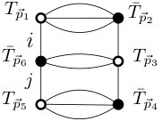 Figure 1
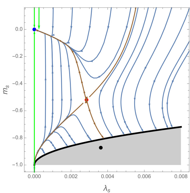 Figure 2
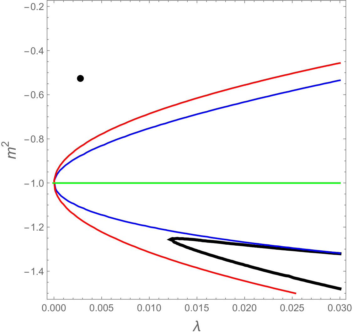 Figure 3
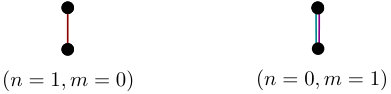 Figure 4
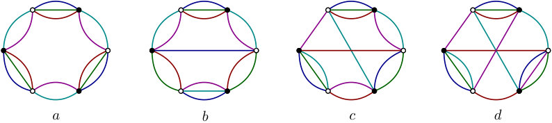 Figure 5
 Figure 6
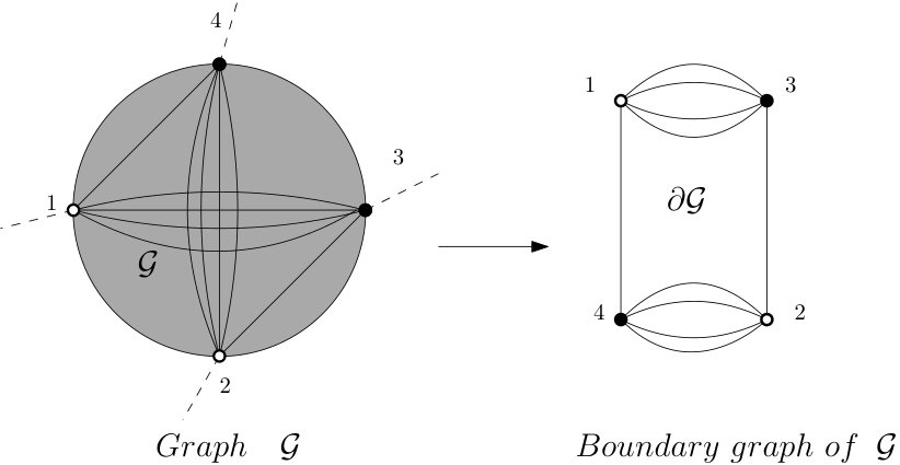 Figure 7
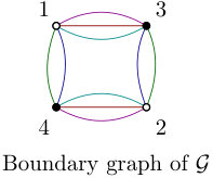 Figure 8
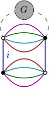 Figure 9
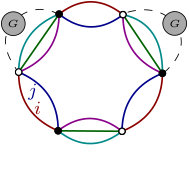 Figure 10
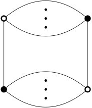 Figure 11
 Figure 12
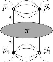 Figure 13
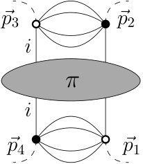 Figure 14
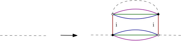 Figure 15
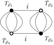 Figure 16
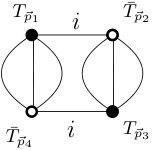 Figure 17
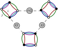 Figure 18
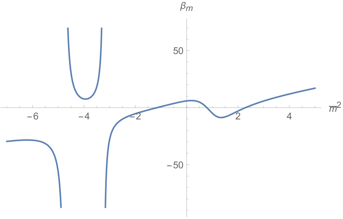 Figure 19
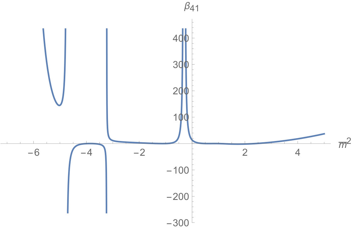 Figure 20
 Figure 21
 Figure 22
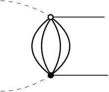 Figure 23
 Figure 24
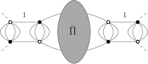 Figure 25
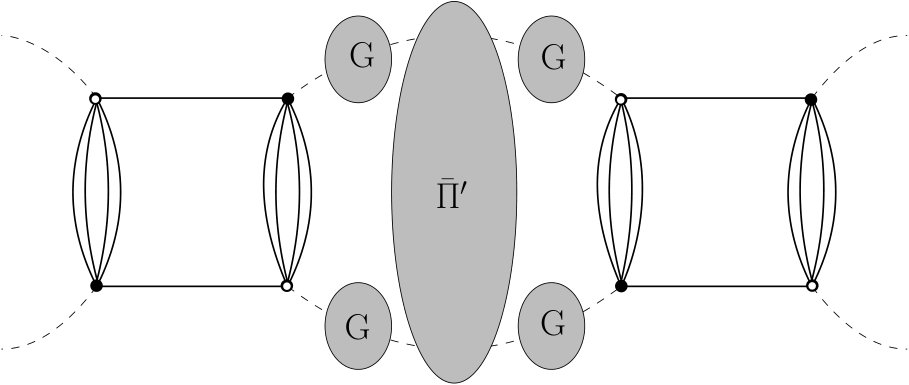 Figure 26
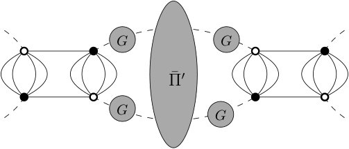 Figure 27
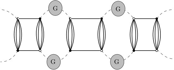 Figure 28
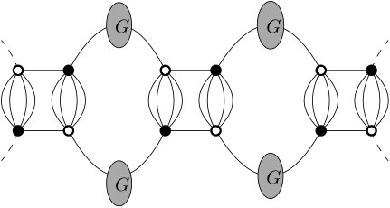 Figure 29
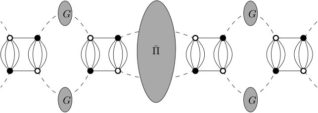 Figure 30
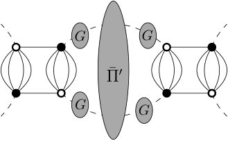 Figure 31
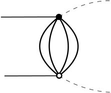 Figure 32
 Figure 33
 Figure 34
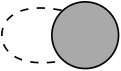 Figure 35
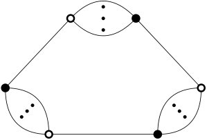 Figure 36
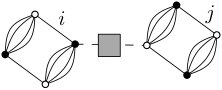 Figure 37
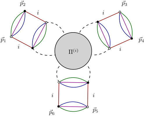 Figure 38
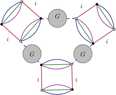 Figure 39
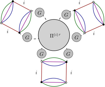 Figure 40
Peer Reviews
No public reviews on file for this paper yet. If you reviewed it on a platform where reviews are public (OpenReview, ICLR, NeurIPS, ICML), you can paste yours below so the community can read it here.
Videos
No videos yet. Explain this paper in a talk, walkthrough, or lecture? Add one.
Progress in Group Field Theory and
Related Quantum Gravity Formalism
**Progress in solving nonperturbative renormalization group for tensorial group field theory **
Vincent Lahochea[email protected], and Dine Ousmane Samarya,b[email protected]
a) Commissariat à l’Énergie Atomique (CEA, LIST), 8 Avenue de la Vauve, 91120 Palaiseau, France
c) Faculté des Sciences et Techniques/ ICMPA-UNESCO Chair, Université d’Abomey- Calavi, 072 BP 50, Benin
Abstract
This manuscript aims at giving new advances on the functional renormalization group applied to the tensorial group field theory. It is based on a series of our three papers [arXiv:1803.09902], [arXiv:1809.00247] and [arXiv:1809.06081]. We consider the polynomial Abelian models without closure constraint. More specifically, we discuss the case of the quartic melonic interaction. We present a new approach, namely the effective vertex expansion method, to solve the exact Wetterich flow equation, and investigate the resulting flow equations, specially regarding the existence of non-Gaussian fixed points for their connection with phase transitions. To complete this method, we consider a non-trivial constraint arising from the Ward-Takahashi identities, and discuss the disappearance of the global non-trivial fixed points taking into account this constraint. Finally, we argue in favor of an alternative scenario involving a first order phase transition into the reduced phase space given by the Ward constraint.
1 Introduction
In seeking a theory to unify modern physics, i.e. a well defined theory of quantum gravity, numerous contributions have been made. Despite the fact that none of them has given a complete resolution to the problem, several major advances have been observed. In the number of these advances, we count the very recent propositions such as loop quantum gravity [1]-[2], dynamical triangulation [3]-[5], noncommutative geometry [6]-[7], group field theories (GFTs) [8]-[12] and tensors models (TMs) [13]-[22]. These approaches are considered as new background independent approaches according to several theoreticians. GFTs are quantum field theories over the group manifolds and are considered as the second quantization version of loop quantum gravity [12]. These theories are caracterized by the specific form of non-locality in their interactions. TMs, especially colored ones, allow one to define probability measures on simplicial pseudo-manifolds such that the tensor of rank represents a -simplex. TMs admit the large -limit ( is the size of the tensor) dominated by the graphs called melons, thanks to the Gurau breakthrough [20]-[22]. The large -limit or the leading order encodes a sum over a class of colored triangulations of the -sphere and its behaviour is a powerful tool which allows us to understand the continuous limit of these models through, for instance, the study of critical exponents and phase transitions. TM and GFT are combined to give birth to a new class of field theories called tensorial group field theory. These class of field models enjoy renormalization and asymptotic freedom [23]-[39]. Using the functional renormalization group (FRG) method, it is also possible to identify the equivalent of Wilson-Fisher fixed point for some particular cases of models.
There are several ways to introduce the FRG in field theories. The first approach is the one pioneered by Wilson, simple and intuitive and therefore yields a powerful way to think about quantum field theories [40]. This method allows a smooth interpolation between the known microscopic laws IR-regime and the complicated macroscopic phenomena in physical systems UV-regime and is constructed with the incomplete integration as cutoff procedure. Well after Polchinski provided a new approach called Wilson-Polchinski FRG equation [41] to address the same question inspired from the Wilson’s method. This very practicable method, which may be integrated with an arbitrary cutoff function and expanded up to the next to leading order of the derivative expansion. Despite the fact that all these approaches seem to be nonperturbative, in practice, the perturbative solution has appeared more attractive. More recently the so called Wetterich flow equation [67], is proposed to study the nonperturbative FRG and this study requires approximations or truncations and numerical analysis which is not very well controlled. The FRG equation allows to determine the fixed points and probably the phase transition. These phase transitions in the case of TGFT models may help to identify the emergence of general relativity and quantum mechanics through the pregeometrogenesis scenario [42]-[45]. Indeed, the way the quantum degrees of freedom are organized to shape a geometric structure which can be identified with a semi-classical space-time is one of the challenges for GFT approach. In the geometrogenesis point of view, the standard space-time geometry is understood as an emergent property, the scenario leading to this geometric limit being assumed quite closed to Bose Einstein condensation in condensed matter physics.
In the recent works [56]-[58] the effective vertex expansion method is used in the context of the FRG. This leads to the definition of new class of equations called structure equations that help to solve the Wetterich flow equations. Taking into account the leading order contribution in the symmetric phase, the non-perturbative regime without truncation can be studied. The Ward-Takahashi (WT) identities is also derived and become a constraint along the flow. Note that the WT-identities are universal for all field theories having a symmetry, and are not specific to TGFT. Therefore all the fixed points must belong inside to the domain of this constraint line, before being considered as an acceptable fixed points. In the case of quartic melonic TGFT models it has been shown that the fixed point occurring from the solution of Wetterich equation violates this constraint for any choice of the regulator function. This violation is also independent of the method used to find this fixed point, whether it is the truncation, or the EVE method. This point will be discussed carefully in this note. Let us remark that most of the TGFT models previously studied in literature are showed to admit at least a non trivial fixed point and therefore a phase transition. The phase transitions are very useful to the likely emergence of metric and are linked to the existence of fixed points, which becomes unavoidable in the search of models which may be probably describe our universe after geometrogenesis scenario. However, in this paper, we study the quartic -TGFT models and prove that no fixed points can be found. First of all we considered the Wilson-Polchinski renormalization group method and show the weakness of this method in the nonperturbative regime. Then we consider the nonperturbative Wetterich flow equation from which the nonperturbative analysis can be made by an approximation on the average effective action called truncation. The EVE method is used to get around the approximation and therefore solves the flow without truncation. The set of Ward-Takahashi identities and structure equations are derived to provide a nontrivial constraint on the reliability of the approximation schemes, i.e. the truncation and the choice of the regulator.
The paper is organized as follows: In section (2) we recall the FGR method by Wilson-Polchinski and apply it in the context of TGFT. Despite the efficiencies of this method, we will present some questions that arise, in the search of a nonperturbative solution and then we will go further in the Wetterich flow equation. Section (3) is dedicated to the description of the Wetterich flow equation and the corresponding solution when the truncation method is applied. We also show that the only nontrivial fixed point which comes from the solution of the flows, violates the Ward identities. In the section (4), we perform new nonperturbative analysis using the so called structure equations is given and the solution of the flow equations are also derived. In the last section (5) we provide a discussion and conclusion to our work.
2 Introduction to the nonperturbative renormalization for TGFT
FRG is a powerful ingredient to think about when it comes to quantum field theories. Generally, in every situation where the scale belong to a range of correlated variables, the theory may be treated by the RG. The first conceptual framework is Wilson’s version of the RG which, by Polchinski, may be applied in the case of quantum field theory. In this section we discuss the nonperturbative renormalization group using not only the Wilson-Polchinski equation but also the Wetterich flow equation. We discuss each method and consider the Wetterich flow equation as more suitable for the treatment of FRG applied to TGFT. Thanks to the Wilson method, the renormalization and renormalization group are understood as a coarse-graining process from a microscopic theory toward an effective long-distance theory. There are in fact different implementations of this idea, depending on the context. In the context of TGFT, we consider the pair of complex fields and which takes values of -copies of arbitrary group :
[TABLE]
In a particular case we assume that is an Abelian compact Lie group. For the rest we only consider the Fourier transform of the fields and denoted by and respectively, written as (for , ):
[TABLE]
The description of the statistical field theory is given by the partition function :
[TABLE]
where is the interaction functional action assumed to be tensor invariant, , the external currents and a shorthand notation for
[TABLE]
The Gaussian measure is then fixed with the choice of the covariance . In this paper, we adopt a Laplacian-type propagator of the form:
[TABLE]
In order to prevent the UV divergences and supress the high momenta contributions, the propagator (5) has to be regularized. In usual case the Schwinger regularization is used:
[TABLE]
In general case, by defining the function such that the condition is fatisfied for and , we can write the propagator as a Laplace transform:
[TABLE]
Then, we shall make the simplest choice , where is the Heaviside function, in order to recover the Schwinger regularization (6). For the rest we keep mind that the propagator is regularized and the infinite limit will be given in an appropriate way. In this case the following result in well satisfied:
Proposition 1**.**
Let us consider two non-normalized Gaussian measures and whose covariances and are related by and such that , and are assumed to be positive. Then we get the following relation:
[TABLE]
where and .
Proof.
The proof of this formula can simply be given using the definition of the Gaussian measure with mean zero and covariance matrix as
[TABLE]
and the fact that
[TABLE]
∎
We introduce tensorial unitary invariants, or simply tensorial invariants. An invariant is a polynomial in the tensor entries and which is invariant under the following action of ( being the size of the tensors):
[TABLE]
The algebra of invariant polynomials is generated by a set of polynomials labelled as bubbles. A bubble is a connected, bipartite graph, regular of degree , whose edges must be colored with a color belonging to the set , and such that all colors are incident at each vertex (and is incident to exactly once). Examples of bubbles are displayed in Fig. 1.
In this paper we consider the quartic melonic model which is proved to be renormalizable in all orders in the perturbative theory. The interaction of this model takin into account the leading order contributions: (melon) is written graphically as:
[TABLE]
Note that the interaction (12) is invariant under the unitary transformations . In contrast, it is not the case for the kinetic terms and sources terms due to the non-trivial propagator and sources and . This implies the existence of a non-trivial Ward-identity which becomes a strong constraint and will be taking into account in the FRG point of view.
2.1 Wilson-Polchinski equation
In this subsection we discuss the Wilson-Polchinski RG equation and provide the corresponding solutions of the quartic melonic TGFT. For this let us introduce a dilatation parameter . This parameter will be used as an evolution parameter in the integration around the UV modes. The RG idea is that if we want to describe the phenomena at scales down to , then we should be able to use the set of variables defined at the scale . Indeed, define the variation
[TABLE]
In the case where is closed to , denoting by the infinitesimal version of the above variation, we get:
[TABLE]
such that the partition function can be written as an integral over two fields, respectively associated to the “slow” and “rapid” modes. Starting with the partition function at scale , we get
[TABLE]
The proposition (1) allows us to decompose into two Gaussian integrals over two fields, and , corresponding respectively to the “rapid” and “slow” modes, with covariances and :
[TABLE]
Then, identifying the effective action at scale as:
[TABLE]
and the decomposition 16 becomes:
[TABLE]
Now, for an infinitesimal step, keeping only the leading order terms in when is very close to , we find:
[TABLE]
with . At the same time, expanding the left hand side of 18 in powers of , and identifying the power of leads to :
[TABLE]
Graphically this equation is given by (and is considered as the Wilson-Polchinski RG equation):
[TABLE]
Note that we may consider not only as a fundamental scale, but also as an arbitrary step on the flow, meaning that the equation 20 holds at each step of the flow. Physically, equation 20 explains how the couplings are affected when the fundamental scale changes, and is therefore the one pioneered idea of the renormalization group flow firstly given by Wilson. This approach follows from a remarkably simple and intuitive idea and yields a very powerful way to think about quantum field theories. The relation (21) can be also expanded in the following result:
Proposition 2**.**
The set of Wilson-Polchinski renormalization group equations are given by
[TABLE]
where , . In this formula we denote by the number of black and white nodes in each interactions and we consider the following expansion for :
[TABLE]
Proof.
A pragmatic way to introduce field strength renormalization is the following. We consider a wave function and the regularized field at the scale . A new functional is associated to this field such as . The equation 20 is then modified into (we deleted the tildes notation):
[TABLE]
Then, by considering the following expansion for :
[TABLE]
we get the relation (22). ∎
The Wilson-Polchinski equation is a leading order equation in the perturbation rather than the loop expansion. Note that we can show that this equation can be turned into a Fokker-Planck equation and therefore may be formally solved by a standard method. The rest of this section is devoted to a perturbative analysis of the flow equations. Before starting this computation, we have to precise the approximation regime. We shall consider only the UV limit which corresponds to the higher values of the scale parameter or to the higher momenta variables or also for the smaller distances, and we assume that and are large. However, the analysis in the UV regime can be extended to IR limit, which corresponds to the smaller values of the scale parameter . More precisely, our approximation can be characterized by both and in the UV and by in the IR. At scale , and up to contributions of order , kipping only the melonic contribution the action providing from (12) is assumed to be of the form
[TABLE]
where the first two terms take into account the fact that the parameter of Gaussian measure, the mass and the Laplacian term, can be affected by the integration of the UV modes, and these counter-terms, assumed to be of order , take into account these modifications. The vertex is a product of delta function and is given by
[TABLE]
Moreover, note that in this approach the corrections to the Laplacian term are not suppressed by an effective counter-term in the action, but absorbed in the wave function renormalization. It is fixed such that all the Laplacian corrections are canceled by the term in the RG equation for . We adopt the standard Ansatz, namely that the generic interaction of valence are of order . This allows to organize systematically the perturbative solution, for which we shall construct the order.
at order
The first corrections occur at order for , whose flow equation write as:
[TABLE]
where
[TABLE]
and and . The r.h.s involves two typical contributions which are pictured graphically in figure 2, where the contraction with is represented by a dotted line with a gray box.
In the UV limit that we consider, the non-melonic contractions of type 2b, creating only one internal face (of color 5 in this figure), can be neglected in comparison to the melonic contributions of the form of figure 2a. Retaining only the melonic contractions, equation 28 becomes:
[TABLE]
with . Expanding this relation in power of , we generate mass and wave function corrections, and also the sub-dominant corrections, involving powers of greater than two. They correspond to the first deviation to the original form 26. Neglecting these sub-dominant contributions, we get the expansion
[TABLE]
for which we only keep the leading order terms in , we can extract the dominant contributions to the mass and wave-function renormalization. The term in generates a non-local 2-point interaction of the form , where is the Laplacian on , and the first term generates a mass correction. Summing over the five colors, we find, at first order in :
[TABLE]
and at order
Let us focus on the second order perturbative solution i.e. at in which we have to take into account the contributions of interactions of valence six, , verifying the flow equation:
[TABLE]
which can be easly integrated with the initial condition as:
[TABLE]
As for the interaction of degree , the structure of this effective interaction can be understood as a contraction between two bubbles, as pictured in figure 3, where the dotted line with a gray box represents the contraction with .
.
Let us now build the effective coupling for the quartic melonic interaction at order , for which we shall extract only the leading behavior. From the Wilson-Polchinski flow equations (22), it seems that the coupling evolution receives many contributions in which the first one comes from . Now deriving two times this interaction with respect to the fields, we obtain an interaction of degree two, which can be either 1PI, when the contraction with links two black and white nodes of two different bubbles, or one particle reducible (1PR) if the two nodes stand on the same interaction bubble. Explicitly we get
[TABLE]
where:
[TABLE]
and
[TABLE]
Equation 35 gives the exact behavior for the beta function at order , but we can easily see that it reduces to the expression of the beta function already obtained for the one loop computation in the deep UV sector. Indeed, retaining only the melonic contributions, and noting that 1PR contributions of the r.h.s are exactly canceled by the term involving the mass correction in the l.h.s, we get:
[TABLE]
The computation of the loop appearing on the r.h.s leads to
[TABLE]
from which we finally deduce that:
[TABLE]
which, as claimed before, is exactly the value of the one-loop beta function already obtained in the one loop computation of the beta function.
We conclude that the main advantage of the Wilson-Polchinski equation is that it provides a very well defined interpretation of the renormalization group flow in the space of couplings. However, except for perturbative computations, the Wilson-Polchinski equation is more adapted to mathematical and formal proofs than to non-perturbative analysis. The analysis beyond the perturbative level requires another formulation of the coarse-graining renormalization group, called Wetterich equation, which allows usually to better capture the non-perturbative effects. The price to pay is an approximation scheme a bit more difficult to use. This non-perturbative approach to the renormalization group flow will be the subject of the next sections.
3 Wetterich flow equation
The Wetterich method and its incarnation into the FRG approach is a set of techniques allowing to go beyond the difficulties coming from the Wilson-Polchinski equation, in particular in regard to track non-perturbative aspects. The Wetterich equation is a first-order functional integro-differential equation for the effective action. The central object of the method is a continuous set of models labelled with a real parameter running from UV scales () to the IR scales (). The physical running scale define for each models what is UV and what is IR, the fluctuation with a large size with respect to the referent scale (the UV fluctuations) being integrated out. The renormalization group equation then describes how the coupling constant change when the referent scale change. To say more, each model is characterized by a specific partition function , labeled by and defined as:
[TABLE]
As a result, the original model corresponds to , and because physically this limit have to match with the IR limit , we require that vanish in the same limit. The term called IR regulator play the same role as a momentum dependent mass term, becoming very large in the UV and vanishing in the IR. It is chosen ultra-local in the usual sense:
[TABLE]
the regulating function being chosen to satisfy the boundary conditions in the UV/IR limit. Moreover, for fixed, aims at freezing the long distance fluctuations, which are discarded from the functional integration. In formula: for , and in the opposite limit.
The object whose we track the evolution is called effective averaged action , defined as (slightly modified version of) the Legendre transform of the standard free energy :
[TABLE]
This definition ensures that satisfies the physical boundary conditions where denote some fundamental UV cutoff. The fields and are the mean values of and respectively and are given by
[TABLE]
where . In general the regulator is chosen to be r_{s}=Z(s)k^{2}f\Big{(}\frac{\vec{p}\,^{2}}{k^{2}}\Big{)},\,\,k=e^{s}, and such that the boundary conditions is well satisfied.such that the boundary conditions in the UV/IR limit are well satisfied. Taking the first derivative with respect to the flow parameter , one can deduce the Wetterich equation, describing the behavior of the effective action when changes:
[TABLE]
where denotes the second order partial derivative of with respect to the mean fields and . This equation is exact, but generally impossible to be solved exactly. A large part of the FRG approach is then devoted to approximate the exact trajectory of the RG flow. In this review, we will discuss two methods, the truncation method, and the effective vertex expansion method.
This section is especially devoted to the truncations. The general strategy is to cut crudely in the full theory space, projecting systematically the flow into the interior of a finite dimensional subspace. To say more, the average effective action is chosen to be of the form:
[TABLE]
where is finite, stands for the interaction function of order and and are the mass and coupling constants. With this truncation and with an appropriate regulator it is possible to solve the Wetterich flow equation (45). In the case of quartic melonic interaction and by taking the standard modified Litim’s regulator:
[TABLE]
the Wetterich equation can be solved analytically and the phase diagram may be given [56]-[57], [58]. The corresponding non trivial fixed points can be studied taking into account the behavior of the flow around these points. Note that the validity of the fixed point require a few analysis taking into account the Ward-Takahashi identities as a new constraint along the flow line. The full violation of this constraint for quartic melonic interaction make this class of fixed points unphysical . We discuss this point in detail in this section (for more detail see subsection (3.1)). The flow equations are
[TABLE]
with the renormalization condition
[TABLE]
where
[TABLE]
Explicitly using the integral representation of the above sum and with , we get
[TABLE]
In order to get an autonomous system, the standard strategy consist at extracting from the couplings the part coming from their own scaling, defining their canonical dimension. Strictly speaking, fields, couplings and all the parameters involved in the theory are dimensionless, because there are no referent space-time, and then not referent scale. The canonical dimension emerge taking into account quantum corrections, and is usually defined as the optimal scaling, with respect to the UV cut-off of the quantum corrections. Conversely, it can be defined as the scaling transformation allowing to get an autonomous system. Note that these two points of views are note strictly equivalent, especially with respect to the choice of the initial content of the theory. For our purpose however, the two strategy provides exactly the same rescaling, and in term of dimensionless parameter , the system (51) becomes
[TABLE]
where , and:
[TABLE]
The solutions of the system (57) is given analytically :
[TABLE]
Numerically
[TABLE]
Apart from the fact that we have a singularity line around the point in the flow equation (51), another second singularity arise from the anomalous dimension denominator, and corresponds to a line of singularity, with equation:
[TABLE]
This line of singularity splits the two dimensional phase space of the truncated theory into two connected regions characterized by the sign of the function . The region , connected to the Gaussian fixed point for and the region for . For , the flow becomes ill defined. The existence of this singularity is a common feature for expansions around vanishing means field, and the region may be viewed as the domain of validity of the expansion in the symmetric phase. Note that to ensure the positivity of the effective action, the melonic coupling must be positive as well. Therefore, we expect that the physical region of the reduced phase space correspond to the region . From definition of the connected region and because of the explicit expression (58), we deduce that :
[TABLE]
Then, only the fixed point is taking into account. In the next subsection we will discuss the violation of the Ward identity around this fixed point , and then clarify our analysis given in [56]. The phase diagram is given in the figure (4)
3.1 Convenient search of the Ward identities
Let , where the are infinite size unitary matrices in momentum representation. We define the transformation:
[TABLE]
such that the interaction term is invariant i.e. Then consider an infinitesimal transformation:
[TABLE]
where is the identity on , the identity on , and denotes skew-symmetric hermitian matrix such that and . The invariance of the path integral (3) means , i.e.:
[TABLE]
Computing each term separately, we get successively using linearity of the operator :
[TABLE]
where , , and . is the renormalized wave function usually denoted by . We get the following result:
Proposition 3**.**
The ward identity gives relation between two and four point functions as:
[TABLE]
where, defined by , the 1PI four point function, we get
[TABLE]
Proof.
The formal invariance of the path integral implies that the variations of these terms have to be compensate by a non trivial variation of the source terms. Combining the two expressions (65), (66), (67) and (68), we come to
[TABLE]
where we have used the fact that, for all polynomial the following identity holds:
[TABLE]
Equation (71) is satisfied for all . Now, expanding each derivative, the partition function of the theory defined by the action (12) verify the following (WT identity),
[TABLE]
WI-identity contains some informations on the relations between Green functions. In particular, they provide a relation between and points functions, which, maybe translated as a relation between wave function renormalization and vertex renormalization . Applying on the left hand side of (73), and taking into account the relations
[TABLE]
as well as the definition G_{s\,,\vec{p}\vec{q}\,}^{-1}:=(\Gamma^{(2)}_{s}+r_{s}\big{)}_{\vec{p}\vec{q}\,}, we find that
[TABLE]
and therefore the proposition (3) is well given. ∎
In the deep UV, for large scale , a continuous approximation for variables is suitable. Then, setting , , , we get finally, in the deep UV, the and -point functions are related as (on both sides, ):
[TABLE]
To give more comment on the structure of this equation, we have to specify the structure of the vertex function. To this end, we use this loop to discard the irrelevant contributions, and we keep only the melonic contribution of the function , denoted by . In the symmetric phase, the melonic contribution may be defined as the part of the function which decomposes as a sum of melonic diagrams in the perturbative expansion. The structure of the melonic diagrams has been extensively discussed in the literature, and specifically for the approach that we propose here in [57]-[58]. Formally, they are defined as the graphs optimizing the power counting; and they family can be build from the recursive definition of the vacuum melonic diagrams, from the cutting of some internal edges. Among there interesting properties, these construction imply the following statement:
Proposition 4**.**
Let be a -point 1PI melonic diagrams build with more than one vertices for a purely quartic melonic model. We call external vertices the vertices hooked to at least one external edge of has :
* two external edges per external vertices, sharing external faces of length one.*
* external faces of the same color running through the interior of the diagram.*
As a direct consequence of the proposition 4, we expect that melonic -points functions is decomposed as:
[TABLE]
the index running from to corresponding to the color of the internal faces running through the interiors of the diagrams building . Moreover the monocolored components have the following structure:
[TABLE]
the permutation of the external momenta and coming from Wick’s theorem: There are four way to hook the external fields on the external vertices (two per type of field). Moreover, the simultaneous permutation of the black and white fields provides exactly the same diagram, and we count twice each configurations pictured on the previous equation. This additional factor is included in the definition of the matrix , whose entries depend on the components of the external momenta running on the boundaries of the external faces of colors , connecting together the end vertices of the diagrams building .
Inserting (78) into the Ward identity given from equation (76), we get some contributions on the left hand side, the only one relevant of them in the deep UV being, graphically:
[TABLE]
Setting , and using the definition of as well as the definition of , the right hand side is reduced to . Moreover, the diagram on the left hand side can be written with the following equation such that the following equality holds:
[TABLE]
where we have defined as:
[TABLE]
Finally, from definition (78) we expect that , and because of the renormalization conditions (52) we must have the relation: . Therefore, in the deep UV regime, the Ward identity between and point functions provides a non trivial relation between effective coupling and wave function renormalization:
[TABLE]
Remark 1**.**
Let us give some important remarks regarding the derivation of the Ward identity (82). First of all, the WI is totally disconnected from the approximation used to solve the non-perturbative Wetterich equation (45). The Wetterich equation and Ward identity are both two functional results, deduced from the definition of the partition function, and have to be treated on the same footing. Their origins, moreover, are completely disconnected. One of them comes from the scale dependence of the model due to the regulator term, the second one comes from the symmetry violation of the action (including source terms) under the group and the formal translation-invariance of the Lebesgue measure. Viewing the set has a continuous family of models, one can say that the Wetterich equation dictate how to move from to whereas the WI are constraints between the observables at fixed .
From now, in the hope to provide the proof that does not live in the constraint line coming from Ward identity (82), let us give the following result which will be prove in the next section.
Proposition 5**.**
Structure equation for effective coupling: In the deep UV, the effective melonic coupling is given in terms of the renormalized coupling and the renormalized effective loop as:
[TABLE]
where we defined the quantity as:
The constraint providing from the Ward identity, which relies the -functions and the anomalous dimension is given by:
[TABLE]
This relation need to be taken into account in the Wetterich flow equation and therefore in the search of fixed point. To prove this relation, let us consider the derivative of with respect to using expression (82) and (83):
[TABLE]
In the above relation we have used the decomposition of . Remark that the Ward identity (82) can be written as where . Then (85) becomes:
[TABLE]
We now use the dimensionless quantities , , such that and reexpressing (86) as:
[TABLE]
where and much be simply compute using the integral representation of the sum. We come to:
[TABLE]
and therefore (84) is well given. It is time to prove that this constraint violate the existence of the fixed point . Let is a arbitrary fixed point of the theory. We get Then the constraint (84) implies that at the point we get
[TABLE]
The particular solution correspond to the Gaussian fixed point. For we have only
[TABLE]
It is clear that the fixed point , violate these constraints i.e. does not satisfied the contraint equation (90). The same conclusion can be made for all choice of the regulator see [56]. Finally it is possible to improve the truncation by using the so called effective vertex expansion. In this case, the fixed point obtained by solving the flow equation also violate the Ward constraint (90). We will study this point in the next section.
4 Effective vertex expansion method for the melonic sector
The effective vertex-expansion described in [56]-[58] allows to establish the structure of the Feynman graphs of our models and leads to the structure equations in the leading order sector. It can help to establish the flow equations without truncation. The Feynman graphs of the colored tensor model are -colored graphs [20]-[22]. For the sake of completeness, we remind here a few facts about these graphs, their representation as stranded graphs and their uncolored version. The graphs that we consider possibly bear external edges, that is to say half-edges hooked to a unique vertex. We denote a colored graph, the set of its internal edges (). A colored graph is said closed if it has no external edges and open otherwise. Let be a -colored graph and a subset of . We note the spanning subgraph of induced by the edges of colors in . Then for all , , a face of colors is a connected component of . A face is open (or external) if it contains an external edge and closed (or internal) otherwise. The set of closed faces of a graph is written (). The structure of the boundary graph of denoted by will be useful in the construction of the leading order contribution which may be considered in the derivative expansion to compute the structure equations and therefore the flow equations.
Definition 1**.**
Consider as a connected Feynman graph with external edges. The boundary graph is obtained from keeping only the external blacks and whites nodes hooked to the external edges, connected together with colored edges following the path drawn from the boundaries of the external faces in the interior of the graph . is then a tensorial invariant itself with blacks (resp. whites) nodes. An illustration is given on Figure (5).
The power counting theorem of these models show that the divergence degree of arbitrary Feynman graph is
[TABLE]
The topological operation on the edge of the graph such as contraction is studied extensively in a lot of literatures. We let the reader consult [20]-[22] and references therein. This operation plays an important role in the power counting theorem and allowed to identify the structure of the graph. It makes the connection between the divergence degree of and the spanning tree denoted by . Let "" is the operation of contraction, we get the following proposition:
Proposition 6**.**
Under the contraction of the spanning tree edge the number of internal faces is invariant i.e. The graph is called the rosette.
Note that the contraction of the edge , which leads to the corresponding graph is such that and the divergent degree of the rosette can be easly computed, using the following formula corresponding to the contraction of -dipole: Then the arbitrary Feynman graph is melonic if its boundary graph have the elementary melon structure i.e. the number of face is maximal:
[TABLE]
Due to the existence of the -expansion of tensors models ( denoting the size of the tensor) which provides in return a topological expansion of the partition function in terms of the generalization of genus called Gurau number , does not yield a topological expansion but rather a combinatorial expansion in terms of the degree of the graph. For a colored closed graph , the degree is such that for the melon .
4.1 Structure equations and compactibility with Ward-identities
The Structure equations is the relations between correlation function and allows to establish a constraint between -functions for mass, interactions couplings and wave function renormalization. These relations are obtained in the deep UV limit (i.e. in the domain ) without any assumption about the -functions and without any truncation of the effective action . The only assumption concern the choice of the initial conditions, ensuring the perturbative consistency of the full partition function. The first structure equation concern the self energy (or 1PI -point functions). It takes place as the closed equation for self energy. 333The rank of the tensors is fixed to , and we denote it by to clarify the proof(s). Let us summarize in the following proposition
Proposition 7**.**
In the melonic sector, the self energy is given by the closed equation which takes into account the effective coupling as:
[TABLE]
In the same way, in the melonic sector, the perturbative zero-momenta 1PI four-point contribution is given by:
[TABLE]
where is defined as:
[TABLE]
* being the effective propagator : Let us recall that and are the counter-terms discarding the UV divergences of the original partition function, the initial conditions in the UV are given such that the classical action contain only renormalizable interactions.
Proof.
Concerning the proof of relation (93) we let the reader to consult the reference [59]. Let us define as the zero momenta melonic -points functions made into the graphs for which two vertices maybe singularized (i.e. by graphs which are at least of order in the perturbative expansion). We have444The notations are similar to the ones used for the previous proof. The context however allows to exclude any confusion.:
[TABLE]
Because of the face connectivity of the melonic diagrams, the boundary vertices may be such that the two internal faces of the same color running on the interior of the diagrams building pass through of them. Then we have the following structure:
[TABLE]
where the grey disk is a sum of Feynman graphs. Note that it is the only configuration of the external vertices in agreement with the assumption that is building with the melonic diagrams. Any other configurations of the external vertices are not melonics. At the lowest order, the grey disk corresponds to propagator lines,
[TABLE]
Note that,the external faces have the same color. Now, we can extract the amputated component of , say (which contains at least one vertex, and is irreducible by hypothesis) extracting the effective melonic propagators connected to the dotted lines linked to . We get:
[TABLE]
At first order, is built with a single vertex, and there are only one configuration in agreement with the melonic structure, i.e. maximazing the number of internal faces. The higher order contributions contain at least two vertices, and the argument may be repeated so that the function appears. Finally we deduce the closed relation:
[TABLE]
This equation can be solved recursively as an infinite sum
[TABLE]
which can be formally solved as
[TABLE]
The loop diagram
maybe easily computed recursively from the definition of melonic diagrams, or directly using Wick theorem for a one-loop computation with the effective propagator . The result is:
[TABLE]
and the proposition is proved.
∎
Note that this construction can be easily cheeked to be compatible with Ward identity, especially in the form (79). Conversely, the last result may be derived directly from the equation (79) and from the closed equation for the -point function (93) (see [58]). To prove these two results we only assume that the classical mean field vanish, we deduce from our previous proof, essentially based on the assumption that the effective vertices are analytic with respect to the renormalized coupling, that the analytic domain cover what we called symmetric phase. In the hope to extract the expression of the counter-terms at all orders and to show that the wave function renormalization and the -points vertex renormalization are the same. We have the following result:
Proposition 8**.**
Choosing the following renormalization prescription:
[TABLE]
where and are the renormalized mass and coupling constant; the counter-terms are given by:
[TABLE]
where denote the melonic self-energy.
Proof.
From Proposition 1, we can get:
[TABLE]
Then, setting , we deduce that
[TABLE]
We now concentrated our self on to and . Without lost of generality, the inverse of the effective propagator has the following structure:
[TABLE]
with the notation: . Then from the renormalization conditions, we have :
[TABLE]
Setting in the closed equation for the -point correlation function, and by deriving with respect to for , we get:
[TABLE]
Using the explicit expression for in (107), we get finally:
[TABLE]
∎
Now, consider the monocolor -points function . If we replace by its expression from Proposition 8, we deduce that
[TABLE]
with the definition: . In other words, we have an explicit expression for the effective coupling ,
[TABLE]
from which we get
[TABLE]
In the above relation we introduce the dot notation
[TABLE]
In proposition 8 we have investigated the relations between counter-terms i.e. we have considered the melonic equations as Ward identities for . Far from the initial conditions, the Taylor expansion of the -point function is written as:
[TABLE]
We call the "physical" or effective mass parameter the first term in the above relation:
[TABLE]
while the coefficient is the effective wave function renormalization and is denoted by i.e.
[TABLE]
Now let us consider the closed equation given in proposition 93. By deriving with respect to and by taking , we get:
[TABLE]
Using equation (115), we can express in terms of the effective coupling , and we get:
[TABLE]
Then we come to the following relation
[TABLE]
At this stage, without all confusion let us clarify that: is the wave function counter-term i.e, whose divergent parts cancels the loop divergences, and whose finite part depend on the renormalization prescription. however is fixing to be for from our renormalization conditions.
4.2 Flow equation from EVE method
There are different methods to improve the crude truncations in the FRG literature. However, their applications for TGFTs remains difficult due to the non-locality of the interactions over the group manifold on which the fields are defined. A step to go out of the truncation method was done recently in [57]-[58] with the effective vertex expansion (EVE) method. Basically, the strategy is to close the infinite tower of equations coming from the exact flow equation, instead of crudely truncate them. To say more, the strategy is to complete the structure equation (83) with a structure equation for , expressing it in terms of the marginal coupling and the effective propagator only. In this way, the flow equations around marginal couplings are completely closed. Note that this approach cross the first hypothesis motivating the truncation: We expect that so far from the deep UV, only the marginal interactions survive, and drag the complete RG flow. Moreover, any fixed point of the autonomous set of resulting equations are automatically fixed points for any higher effective melonic vertices building from effective quartic interactions. Finally, a strong improvement of this method with respect to the truncation method, already pointed out in [57]-[58] is that it allows to keep the complete momenta dependence of the effective vertex. This dependence generate a new term on the right hand side of the equation for , moving the critical line from its truncation’s position.
Let us consider the flow equation for , obtained from (45) deriving with respect to and :
[TABLE]
where we discard all the odd contributions, vanishing in the symmetric phase. Deriving on both sides with respect to , and setting , we get:
[TABLE]
where the "prime" designates the partial derivative with respect to . In the deep UV () the argument used in the -truncation to discard non-melonic contributions holds, and we keep only the melonic diagrams as well. Moreover, to capture the momentum dependence of the effective melonic vertex and compute the derivative , the knowledge of is required. It can be deduced from the same strategy as for the derivation of the structure equation (83), up to the replacement :
[TABLE]
from which we get:
[TABLE]
The derivative with respect to may be easily performed, and from the renormalization condition (52), we obtain:
[TABLE]
and the leading order flow equation for becomes:
[TABLE]
As announced, a new term appears with respect to the truncated version (51), which contains a dependence on and then move the critical line. The flow equation for mass may be obtained from (124) setting on both sides. Finally, the flow equation for the marginal coupling may be obtained from the equation (45) deriving it twice with respect to each mean field and . As explained before, it involves at leading order, and to close the hierarchy, we use the marginal coupling as a driving parameter, and express it in terms of and only. One again, from proposition 4, have to be split into monocolored components :
[TABLE]
The structure equation for may be deduced following the same strategy as for , from proposition (4). Starting from a vacuum diagram, a leading order -point graph may be obtained opening successively two internal tadpole edges, both on the boundary of a common internal face. This internal face corresponds, for the resulting -point diagram to the two external faces of the same colors running through the interior of the diagram. In the same way, a leading order -point graph may be obtained cutting another tadpole edge on this resulting graph, once again on the boundary of one of these two external faces. The reason this works is that, in this may, the number of discarded internal faces is optimal, as well as the power counting. From this construction, it is not hard to see that the zero-momenta vertex function must have the following structure (see [57]-[58] for more details):
[TABLE]
the combinatorial factor coming from permutation of external edges. Translating the diagram into equation, and taking into account symmetry factors, we get:
[TABLE]
with:
[TABLE]
Note that this structure equation may be deduced directly from Ward identities, as pointed-out in [58] and [59]. The equation closing the hierarchy is then compatible with the constraint coming from unitary invariance. The flow equations involve now some new contributions depending on two sums, and , defined without regulation function . However, they are both power-counting convergent in the UV, and the renormalizability theorem ensures their finitness for all orders in the perturbation theory. For this reason, they becomes independent from the initial conditions at scale for ; and as pointed out in [58],we get, using the Litim’s regulator:
[TABLE]
and
[TABLE]
The complete flow equation for zero-momenta -point coupling write explicitly as:
[TABLE]
Keeping only the melonic contributions, we get finally the following autonomous system by using the Litim’s regulation:
[TABLE]
where the anomalous dimension is then given by:
[TABLE]
The new anomalous dimension has two properties which distinguish him from its truncation version. First of all, as announced, the singularity line moves toward the axis, extending the symmetric phase domain. In fact, the improvement is maximal, the critical line being deported under the singularity line . In standard interpretations [57], the presence of the region is generally assumed to come from a bad expansion of the effective average action around vanishing means field, becoming a spurious vacuum in this region.
However the EVE method show that the singularity line obtained using truncation is completely discarded taking into account the momentum dependence of the effective vertex. The second improvement come from the fact that the anomalous dimension may be negative, and vanish on the line of equation , with:
[TABLE]
Interestingly, there are now two lines in the maximally extended region where physical fixed points are expected. However, numerical integrations, show that the improved flow equations admit a non-Gaussian fixed point , which is numerically very close from the fixed point obtained in the truncation method i.e. , and then unphysical as well. The other solutions are:
[TABLE]
For we have . This fixed point cannot be taking into account by considering all the explanation given in the section (2). have the following critical exponent , . This fixed point is IR attractive and lives in the same region like . Finally all the fixed point discovered from EVE method violate the Ward identities.
4.3 Exploration of the physical phase space
In this section we will show that the EVE method leads to an alternative first order phase transition scenario, despite the fact that the fixed point is discarded. In the second time we also prove that this new behavior is only observed using EVE method and can not be obtained by implementing the usual truncation as approximation.
1) Despite the fact that the constraint equation (84) is not compatible with the fixed point , this is not the end of the history. The constraint given by equation (84) define a one-dimensional subspace, say into the whole bi-dimensional phase space . Obviously, the Ward identity will be violated everywhere except along this one-dimensional subspace ; for this reason we call physical phase space this subspace.
Solving with respect to , we can extract the coupling constant as function of the renormalized mass parameter . After a few handing computation, we get:
[TABLE]
These solutions provides only one non-trivial parametrized equation for the physical subspace : . Interestingly, it is not hard to cheek that the presence of the factor in the numerator cancel all the formal divergences occurring for , such that the flow becomes regular at this point. However, other divergences occurs, one of them being common to each beta functions. To understand the structure of the effective flow into the physical subspace, we have to insert the solutions (144) into the flow equations (140). However, even to do this, let us discuss the solution (144) in a few words. Because the theory is asymptotically free, we may expect that and have to vanish simultaneously. What we know is that, in the vicinity of the Gaussian fixed point , the constraint is approximately satisfied. For instance, up to contributions, the equation (84) reduces as:
[TABLE]
which is identically satisfied from the one-loop beta equation – see (140). As a result, in a small domain around , the flow behaves approximately according the Ward constraint, but as soon as the flow leaves this region, the Ward constraint is violated, except along the , where it hold strictly. Note that, for , the value of is so large (), and far away from the vicinity of the Gaussian fixed point.
Now, let us move on to the solutions (144). The solution corresponds to trivial flow, and:
[TABLE]
On the other hand, inserting the non-trivial solution , we get:
[TABLE]
and :
[TABLE]
[TABLE]
[TABLE]
As announced, the divergences at the value has been discarded. However, some new divergences occurs. First of all, the equation for becomes singular for the value . This singularity comes from the denominator of . Note that is such that for the small , and , . This singularity is reminescent to the first order phase transition. A second singularity occurs for the values , , which is common for , and . We now discuss this picture. To this end, let us examine the points at which the beta function vanish. We get:
[TABLE]
[TABLE]
Because , we recover our previous conclusion, in the whole theory space , no fixed point can be found using the exact FRG with the EVE method taking into account the Ward constraint. Finally at the point on the projected phase space , the discontinuity of implies the discontinuity of the effective action . The flow into the physical phase space change the direction at this point, pointing toward positive mass direction for and toward the negative mass direction for . In the last case, the flow continues on this way and reaches the singularity, where the flow becomes undefined. Both, these two features are reminiscent of a first order phase transition on the physical phase space – the singularity may indicate a point at which the effective action becomes undefined, or where the expansion around the null vacuum fails to exist – the last statement having to be rigorously investigated.
The same analysis may be performed when we consider the following prescription: by extracting the mass parameter as function of the constant : in the constraint equation and solve the -function of the coupling. In this case, the coupling becomes the parameter, and for the points and we get a singularity corresponding to the values , (see Figure (7)b). Note that around , the coupling becomes very small :
[TABLE]
and we reach a new perturbative regime for small and small .
2) When we investigated the truncation method, we do not performed such a discussion. To compare the methods, let us consider the same strategy for the phase space described with the truncation method. Solving the constraint , we get:
[TABLE]
By replacing this solution in the flow equations of mass and coupling (51) we get
[TABLE]
Now setting , only the Gaussian fixed point survives. Also the last solution leads to
[TABLE]
One more time, we recover that no solutions such that exist. Moreover, we recover that vanish for a negative mass value, not so far from ; and that the singularity at this value has been completely discarded from the solution of the Ward constraint. However, the common singularity of the beta functions as some other aspects of the previous flow equations are not reproduced in the truncation framework. The nature of the singularities, for , remains mysterious in our formalism. Obviously they are a consequence of the improvement coming from the EVE method, and their understanding may be increasing our knowledge about the behavior of the TGFT renormalization group flow.
5 Conclusion
In this manuscript we have studied with different methods the FRG applied to TGFT. First we have derived the Wilson-Polchinski equation and given the perturbative solution. In the second time we derived the Wetterich flow equation using the usual approximation called truncation. The analytic solution of this equation is given. We get a fixed point denoted by . Then we investigated the Ward identities as a new constraint along the flow and showed that the fixed point violates this constraint. Finally we improve the study of FRG by replacing the truncation method by the so called EVE. The flow equation is improved and the corresponding solution is not so far from i.e. . However, the Ward identities are strongly violated at this fixed point and therefore this unique fixed point seems to be unphysical. We have also showed the importance of EVE method in the sense that, despite the fact that the fixed point needs to be discarded, a first order phase transition exists so far from this point in the subspace of the theory space. We have showed that this new behavior can not be observed using the truncation as approximation.
In this review we focus on the EVE method for the melonic approximation, and especially on the quartic melonic just-renormalizable sector. The complete quartic sector, including all the connected quartic bubbles has already been considered in a complementary work [57], and the conclusion about the incompatibility with nonperturbative fixed points and Ward identities hold. The graphs added to the quartic melonic ones to complete the quartic sector have been called pseudo-melons due to the similarities of their respective leading order Feynman graphs. Finally, even if we expect that some aspects of the EVE method improve the standard truncation method, some limitations have to be addressed for future works. In particular our investigations are limited on the symmetric phase, ensuring convergence of any expansion around vanishing classical means field. Moreover, we have retained only the first terms in the derivative expansion of the 2-point function and only considered the local potential approximation, i.e. potentials which can be expanded as an infinite sum of connected melonic (and pseudo-melonic) interactions. Finally, a rigorous investigation of the behavior of the renormalization group flow into the physical phase space has to be addressed in the continuation of current works on this topic.
The reference list from the paper itself. Each links out to its DOI / PubMed record.
- 1[1] C. Rovelli, “Loop quantum gravity,” Living Rev. Rel. 1 , 1 (1998) doi:10.12942/lrr-1998-1 [gr-qc/9710008].
- 2[2] C. Rovelli and P. Upadhya, “Loop quantum gravity and quanta of space: A Primer,” gr-qc/9806079.
- 3[3] J. Ambjorn, Z. Burda, J. Jurkiewicz and C. F. Kristjansen, “Quantum gravity represented as dynamical triangulations,” Acta Phys. Polon. B 23 , 991 (1992).
- 4[4] J. Ambjorn, “Quantum gravity represented as dynamical triangulations,” Class. Quant. Grav. 12 , 2079 (1995). doi:10.1088/0264-9381/12/9/002
- 5[5] J. Ambjørn, A. Görlich, J. Jurkiewicz and R. Loll, “Quantum Gravity via Causal Dynamical Triangulations,” doi:10.1007/978-3-642-41992-8-34 ar Xiv:1302.2173 [hep-th].
- 6[6] A. Connes and J. Lott, “Particle Models and Noncommutative Geometry (Expanded Version),” Nucl. Phys. Proc. Suppl. 18B , 29 (1991). doi:10.1016/0920-5632(91)90120-4
- 7[7] J. Aastrup and J. M. Grimstrup, “Intersecting connes noncommutative geometry with quantum gravity,” Int. J. Mod. Phys. A 22 , 1589 (2007) doi:10.1142/S 0217751 X 07035306 [hep-th/0601127].
- 8[8] D. Oriti, “A Quantum field theory of simplicial geometry and the emergence of spacetime,” J. Phys. Conf. Ser. 67 , 012052 (2007) doi:10.1088/1742-6596/67/1/012052 [hep-th/0612301].