Fisher-Shannon complexity analysis of high-frequency urban wind speed time series
Fabian Guignard, Dasaraden Mauree, Michele Lovallo, Mikhail Kanevski,, Luciano Telesca

TL;DR
This study applies Fisher-Shannon analysis to high-frequency urban wind speed data at various heights, revealing height-dependent complexity and correlations with temperature variability, enhancing understanding of urban wind dynamics.
Contribution
It introduces the use of Fisher-Shannon complexity analysis to examine how urban wind speed variability changes with height and its relation to ambient temperature.
Findings
Fisher-Shannon complexity decreases with height.
Complexity correlates with temperature variance, especially near ground.
Wind variability is influenced by ambient temperature near the surface.
Abstract
1Hz wind time series recorded at different levels (from 1.5 to 25.5 meters) in an urban area are investigated by using the Fisher-Shannon (FS) analysis. FS analysis is a well known method to get insight of the complex behavior of nonlinear systems, by quantifying the order/disorder properties of time series. Our findings reveal that the FS complexity, defined as the product between the Fisher Information Measure and the Shannon entropy power, decreases with the height of the anemometer from the ground, suggesting a height-dependent variability in the order/disorder features of the high frequency wind speed measured in urban layouts. Furthermore, the correlation between the FS complexity of wind speed and the daily variance of the ambient temperature shows similar decrease with the height of the wind sensor. Such correlation is larger for the lower anemometers, indicating that ambient…
Click any figure to enlarge with its caption.
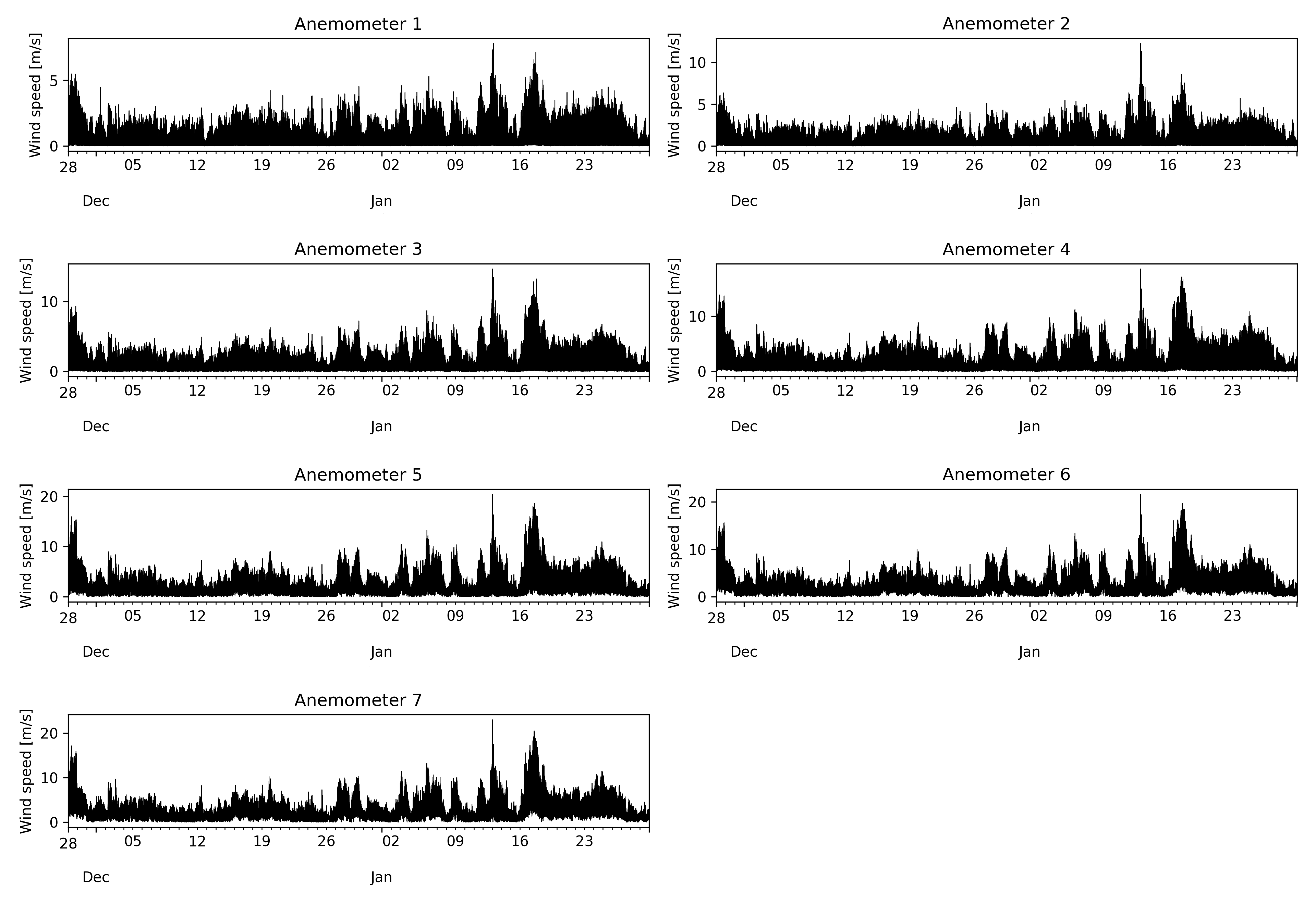 Figure 1
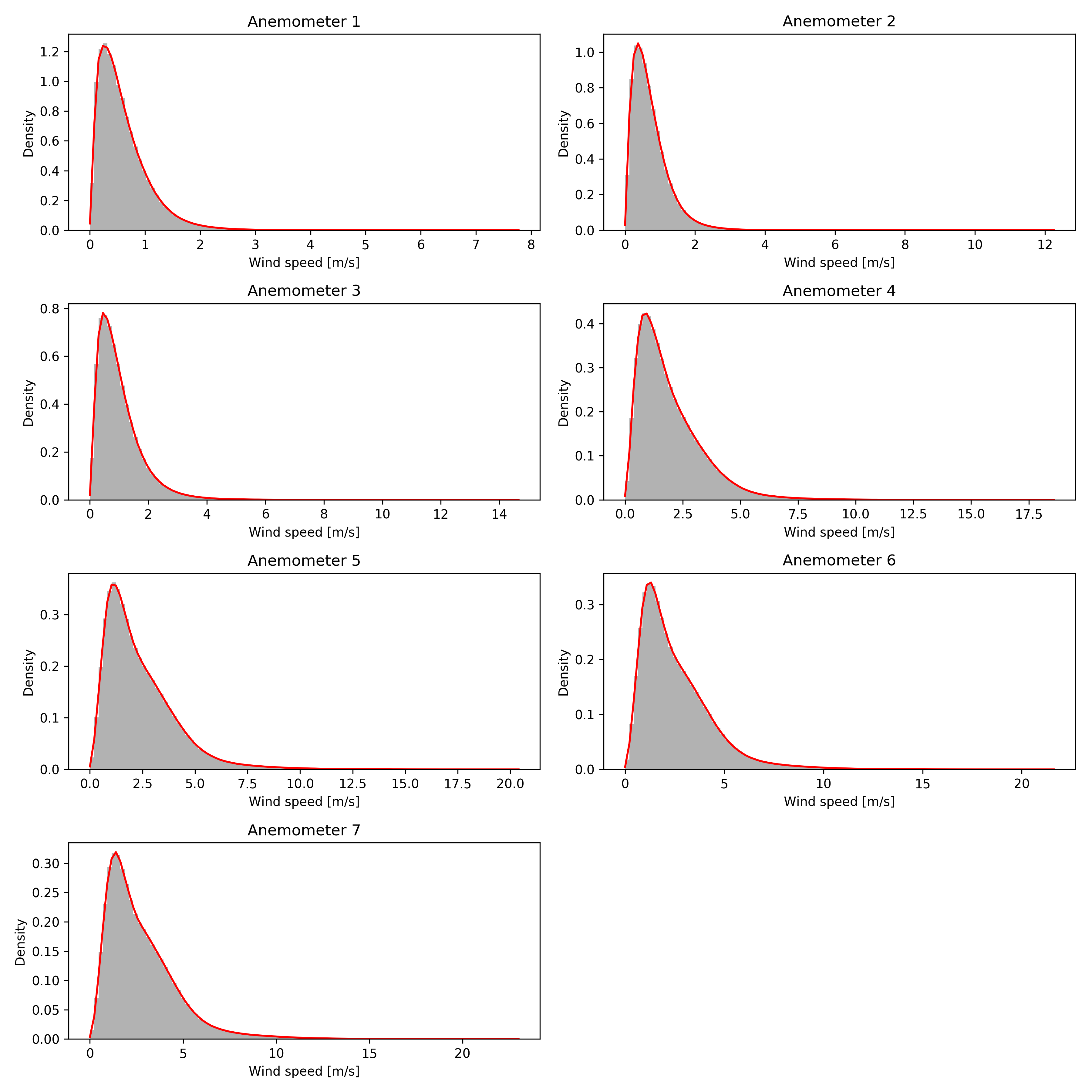 Figure 2
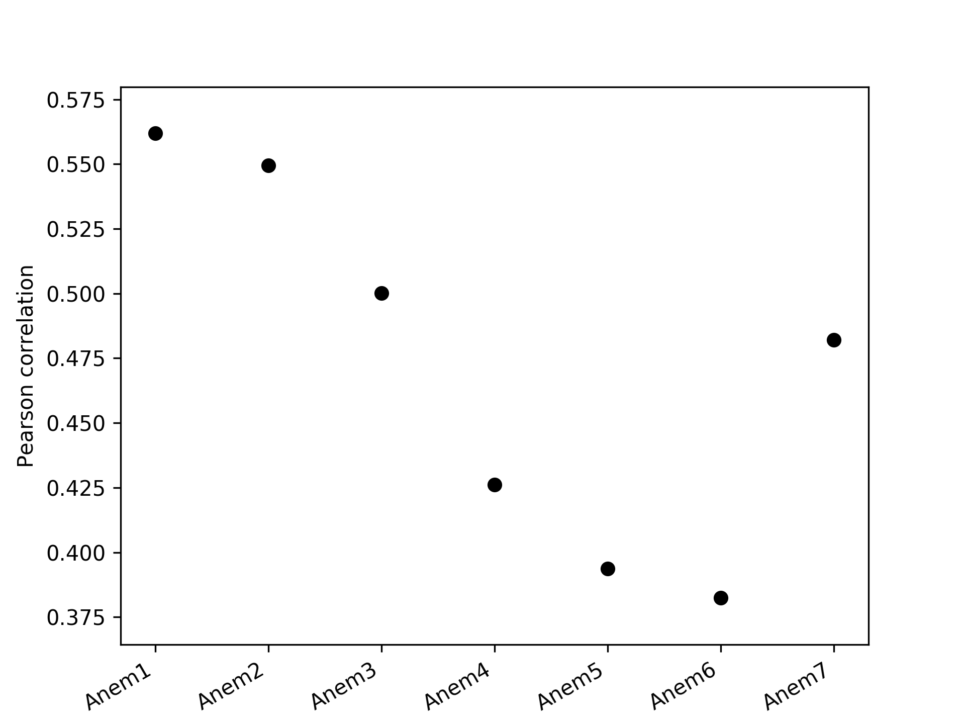 Figure 3
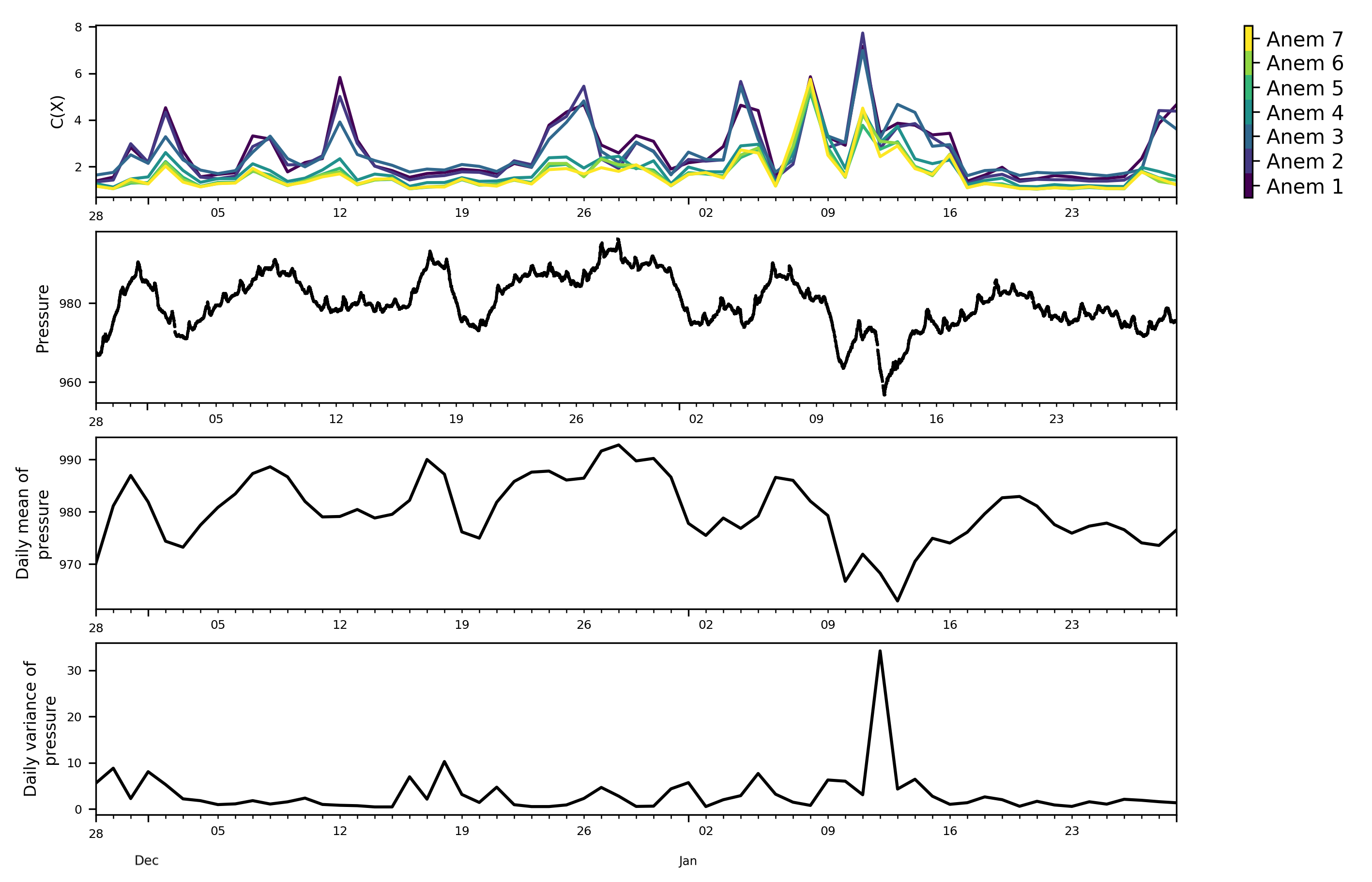 Figure 4
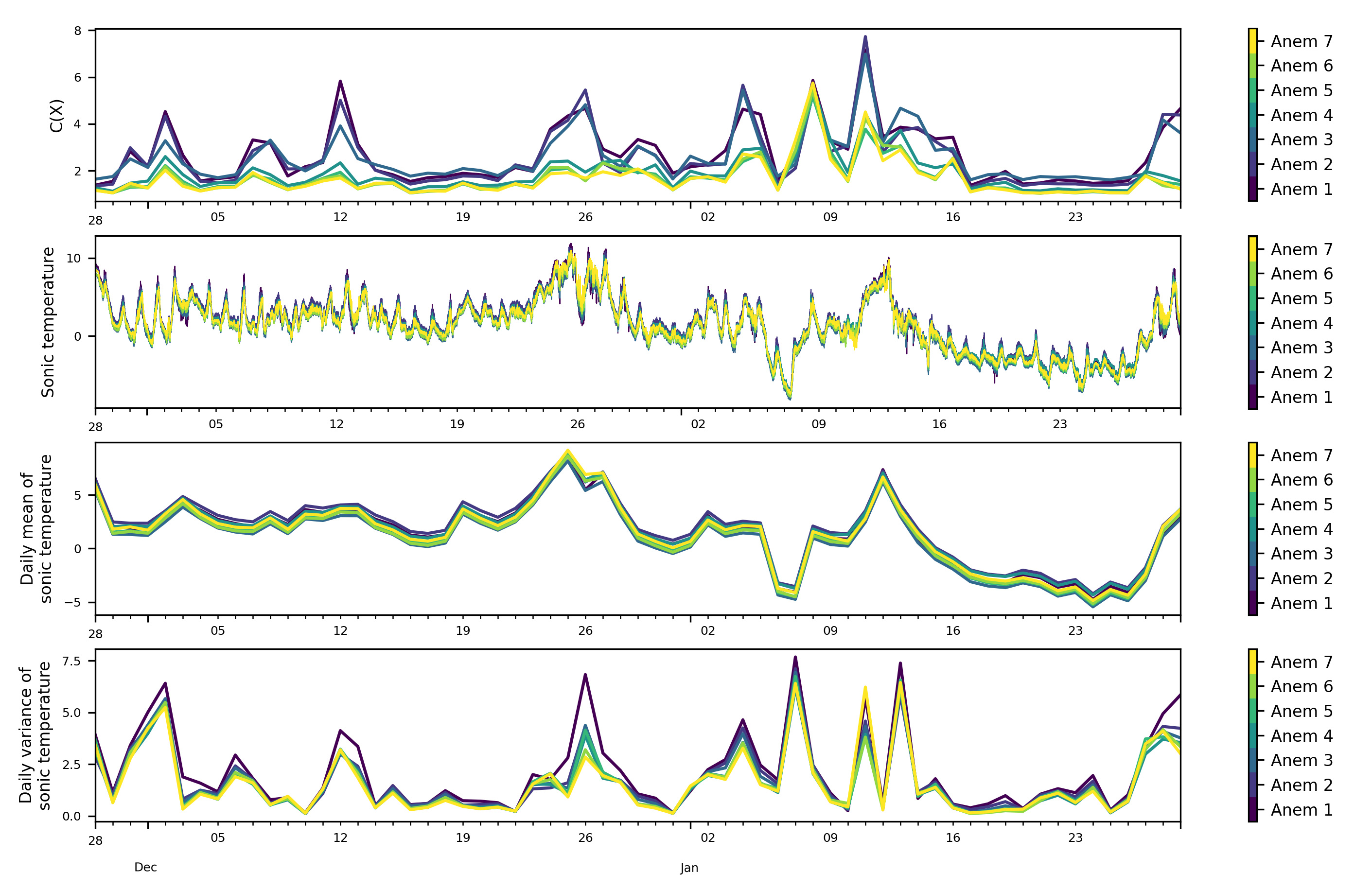 Figure 5
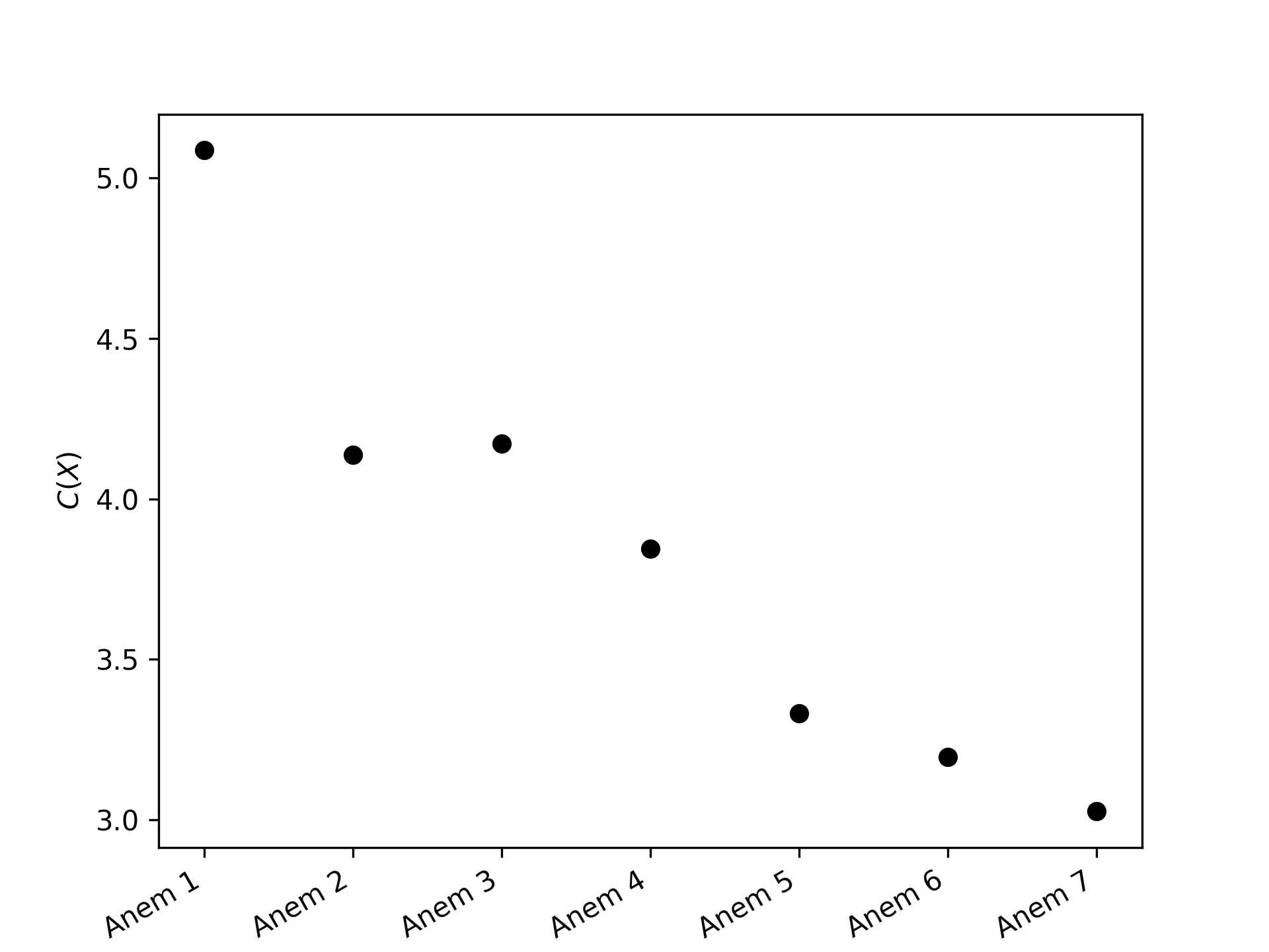 Figure 6
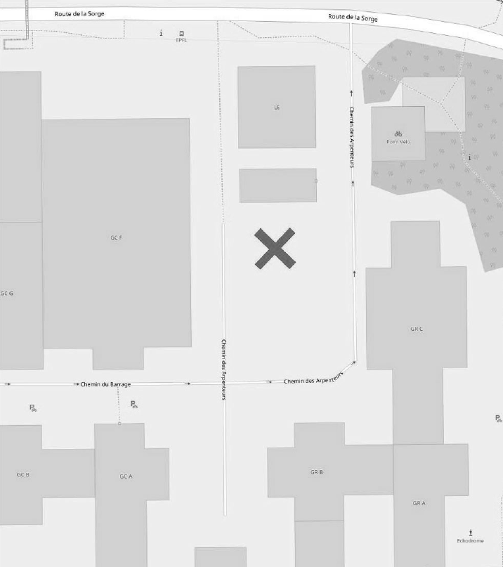 Figure 7
| An 1 | An 2 | An 3 | An 4 | An 5 | An 6 | An 7 | |
|---|---|---|---|---|---|---|---|
| Min. | 0.000 | 0.000 | 0.000 | 0.000 | 0.000 | 0.000 | 0.010 |
| 1st Qu. | 0.278 | 0.351 | 0.481 | 0.920 | 1.173 | 1.280 | 1.395 |
| Median | 0.493 | 0.602 | 0.824 | 1.575 | 1.965 | 2.124 | 2.295 |
| Mean | 0.606 | 0.721 | 1.009 | 1.932 | 2.388 | 2.574 | 2.756 |
| 3rd Qu. | 0.812 | 0.955 | 1.324 | 2.603 | 3.200 | 3.435 | 3.661 |
| Max. | 7.774 | 12.254 | 14.659 | 18.583 | 20.397 | 21.611 | 23.010 |
| Correlation | p - value | |
|---|---|---|
| Anem 1 | 0.562 | 0.001 |
| Anem 2 | 0.550 | 0.001 |
| Anem 3 | 0.500 | 0.001 |
| Anem 4 | 0.426 | 0.002 |
| Anem 5 | 0.394 | 0.002 |
| Anem 6 | 0.382 | 0.006 |
| Anem 7 | 0.482 | 0.001 |
Peer Reviews
No public reviews on file for this paper yet. If you reviewed it on a platform where reviews are public (OpenReview, ICLR, NeurIPS, ICML), you can paste yours below so the community can read it here.
Videos
No videos yet. Explain this paper in a talk, walkthrough, or lecture? Add one.
Abstract
wind time series recorded at different levels (from 1.5 to 25.5 meters) in an urban area are investigated by using the Fisher-Shannon (FS) analysis. FS analysis is a well known method to get insight of the complex behavior of nonlinear systems, by quantifying the order/disorder properties of time series. Our findings reveal that the FS complexity, defined as the product between the Fisher Information Measure and the Shannon entropy power, decreases with the height of the anemometer from the ground, suggesting a height-dependent variability in the order/disorder features of the high frequency wind speed measured in urban layouts. Furthermore, the correlation between the FS complexity of wind speed and the daily variance of the ambient temperature shows similar decrease with the height of the wind sensor. Such correlation is larger for the lower anemometers, indicating that ambient temperature is an important forcing of the wind speed variability in the vicinity of the ground.
keywords:
High frequency wind speed measurments; Fisher-Shannon complexity; Time series; Urban areas
\pubvolume
xx \issuenum1 \articlenumber5
\historyReceived: date; Accepted: date; Published: date \continuouspagesyes \TitleFisher-Shannon complexity analysis of high-frequency urban wind speed time series \AuthorFabian Guignard *1,**, Dasaraden Mauree 2, Michele Lovallo 3, Mikhail Kanevski 1 and Luciano Telesca 4 \AuthorNamesFabian Guignard, Dasaraden Mauree, Michele Lovallo, Mikhail Kanevski and Luciano Telesca
\corresCorrespondence: [email protected]
1 Introduction
When designing urban areas, it is fundamental to consider multiple meteorological parameters. In particular, the buildings and the layout of the urban spaces will strongly impact the pedestrian comfort, building energy use Mauree et al. (2017, 2018), dispersion of air pollutants, and renewable energy potential in urban planning scenarios Perera et al. (2018) due to the wind flow around the built-up spaces. Therefore, there is a need to understand better the influence of the obstacles (buildings, trees, street equipment) on the airflow. This can only be achieved with high quality and high frequency wind data that are registered through experimental campaigns and field trips. Classical meteorological or climatic stations do not measure the wind speeds and direction with a sufficiently high vertical resolution and high frequency. The BUBBLE Rotach et al. (2005) campaign in the early 2000 provided useful data for development and generalization of new parameterization schemes. However, one urban configuration and such a short observation period is not enough to generalize formulations and to understand the underlying physical processes. For instance, to determine the momentum and heat fluxes, it is necessary to measure the vertical profiles of wind speed near buildings Mauree et al. (2017); Järvi et al. (2018); Santiago et al. (2007). Additionally, urban configurations are often characterized by small scale turbulence Christen et al. (2009). Only high frequency wind speed data allow to identify such turbulence.
The complexity of the wind speed in urban areas can be related to the nonlinear interactions that take place at any timescale between the average wind speed vertical gradient, turbulent processes, shape, size and setting of buildings, etc. Hence, robust statistical methodologies are necessary to better characterize the time variability of wind speed in urban areas at different heights from the ground Mauree et al. (2017a, b). The presence of heterogeneous artificial or natural surfaces close to the ground significantly increases the complexity of the turbulent structure. As an example, the high density of vertical surfaces and the ground heating could lead to the development of thermal instabilities.
In this study we investigate the properties of order/disorder in the time variability of seven urban wind speed time series measured at different level from the ground (from 1.5 m to 25.5 m, with 4 m spacing between each anemometer), on a 27 m high mast located in the campus of Ecole Polytechnique Fédérale de Lausanne (EPFL), Switzerland (motus.epfl.ch). The average height of the building layout around the mast is about 10 m Mauree et al. (2017a, b), see Fig. 1. The experiment was performed with the aim to quantitatively evaluate how urban buildings could impact the wind. Building layouts generally cause local turbulence phenomena in the wind flow below the average height of the buildings. Thus, the main goal of the experiment was to discriminate between the turbulent dynamics of wind speed recorded by the anemometers installed below the average building height from the “free flow” dynamics of wind speed recorded by the anemometers placed above. To this aim, in the present research the Fisher-Shannon method is used. This method jointly uses both Fisher information and Shannon entropy on time series. Fisher-Shannon analysis has some useful applications, e.g. it allows to detect non-stationarity Vignat and Bercher (2003) and leads to a measure of complexity Esquivel et al. (2010).
The paper is organized as follows. First, a brief description of the experiment is presented. Then the Fisher-Shannon method is explained. Next, the results are discussed, and the final remarks are summarized in the conclusions.
2 Description of the experiment
A meteorological mast of 27 m high, where seven sonic anemometers (Gill Wind Master) are located each 4m, has been installed in the EPFL campus. The first anemometer is mounted at 1.5 m (corresponding to the average height of the center of an adult) while the last one is at 25.5 m above the ground. It can be noted that the highest sensor was placed far enough above the building layout height to be in the inertial layer Rotach (1999). The three velocity components, the sonic speed and temperature were measured. The frequency of the data is Kaimal and Finnigan (1994). In this study the wind speed and the sonic temperature are analyzed for each level on the tower. The atmospheric pressure is measured at the site, with a Gill meteorological station (GMX300), also with a frequency of . The time series of the wind speed data, collected during two months period from 28 December 2016 to 29 January 2017, are shown in Fig. 2. Fig. 3 shows histograms along with kernel density estimations Parzen (1962); Rosenblatt (1956). Summary statistics are given in Table 1.
3 The Fisher-Shannon analysis
The Fisher-Shannon (FS) method is based on the analysis of two quantities, namely, the Fisher Information Measure (FIM) and the Shannon Entropy Power (SEP).
Let be a random variable and is its probability density function (pdf). FIM of is the real number defined as Cover and Thomas (2006)
[TABLE]
FIM quantifies the amount of organization in the data. SEP of is the real number, noted , defined as E. (1948)
[TABLE]
where is the differential entropy of given by
[TABLE]
SEP is a measure of disorder in data.
Note that FIM and SEP only depend on the pdf , which requires to be estimated. This estimation is performed by the kernel density estimator approach Devroye (1987) : for a given time series of length ,
[TABLE]
where is the bandwidth, and is the kernel function, which is assumed to be continuous, non-negative, symmetric around zero and satisfying the following two constrains
[TABLE]
The computation is carried out by combining the algorithms from Troudi et al. (2008) and Raykar and Duraiswami (2006), which use a Gaussian kernel with zero mean and unit variance :
[TABLE]
Although there is no consensus about the definition of the complexity, FS analysis has been employed as a statistical complexity measure Esquivel et al. (2010); Angulo et al. (2008).
The FS complexity is defined as the product of FIM and SEP,
[TABLE]
It can be shown that , with equality if and only if is a Gaussian random variable Dembo et al. (1991), which is known as the isoperimetric inequality for entropies. Moreover, it is easy to show Vignat and Bercher (2003) that for any scalar ,
[TABLE]
In particular, the FS complexity of a random variable is constant under scalar multiplication.
4 Results and discussion
For each series, the FIM, the SEP, and the FS complexity are calculated. The FS complexity for each anemometer is shown in Fig. 4. It is evident that there is a decreasing pattern of the FS complexity with height increasing from the ground. The largest value is reached at the anemometer placed at 1.5 m and the smallest for the one placed at 25.5 m.
The daily variation of the FS complexity (top of Fig. 5) reveals a clustering tendency among the seven anemometers: the lowest three anemometers are generally characterized by larger values of FS complexity during all the investigation period, while the four highest ones display smaller values of FS complexity through time. It is interesting to note that the lowest three anemometers are placed at height lower than the average height of the buildings surrounding the mast, while the four highest anemometers are placed well above the building average height. It is reasonable to think that such clustering of the wind series into two groups could reflect the different dynamics of the wind flow below and above the average height of the building layout Coceal and Belcher (2004); Christen et al. (2007); Mauree et al. (2017); Oke et al. (2017). However, all curves of the daily variation of FS complexity show a certain coincidence of the occurrences of the peaks, especially in the last half of the investigation period.
To see if any link could be found between the daily variations of the FS complexity with meteo-climatic variables, the daily mean and variance of the ambient pressure (Fig. 5) and sonic temperature (Fig. 6) are calculated. Showing synoptically the daily variation of the FS complexity and the daily variation of the mean pressure and sonic temperature, we can observe that most of the peaks of the FS complexity seem to have a qualitative correspondence with those of the mean pressure, while no apparent correlation with the sonic temperature mean is observed.
The analysis of the correlations between the FS complexity and the variance of pressure and sonic temperature, instead, shows an apparent larger correlation between the FS complexity and the variance of sonic temperature, especially for the lower anemometers. Fig. 7 shows that the Pearson correlation coefficients between the FS complexity and the variance of the sonic temperature is larger for the lower anemometers and smaller for the higher ones. Since the data are non-normal, a non-parametric permutation test is performed for each anemometer in order to assess the significance of the correlation coefficients Davison and Hinkley (1997). The number of permutation is set to . The results are presented in Table 2.
The analysis conducted in this study can suggest two driving forces. The atmospheric pressure obviously indicates the variation in the synoptic flows, hence gives an indication of the general weather condition during the monitoring period. While looking at the variance, the sonic temperature seems to demonstrate that the variation of the temperature has a non-negligible effect on the complexity found in the wind speed (at least inside the canyon). The impact of the radiation and the differential heating of the surfaces inside the urban canyon could also lead to the increased variances Oke et al. (2017).
5 Conclusions
An analysis of the time series of the wind speed from seven anemometers, located in an urban area on a 27 m mast at EPFL, were conducted by means of the Fisher-Shannon methods. The objective of this study was to determine the possible physical causes of the variability in the time series but in the vertical profile of the wind. In particular, the Fisher Information Measure and the Shannon Entropy Power were applied. The study clearly demonstrated that there was a significant decrease in the complexity with height. This confirmed that the presence of buildings and more generally of obstacles in the street canyon, considerably modify the wind structure and profiles in an urban setup. Additionally, the temperatures from the anemometers as well as the atmospheric pressure from an on-site meteorological station were also used to provide data on the prevailing conditions during the monitoring campaign. It appears that the atmospheric pressure could be a proxy for the synoptic flows and the current meteorological conditions. On the other hand, the temperature is a reflection of the amount of heat brought by general flow but also due to the heated surfaces in the canyon. This clearly points to the importance of new parameterization, particularly for the turbulent buoyancy term, as shown in Mauree et al. (2017). Further development will include an analysis of the atmospheric stability while taking into account also the surface temperatures of the surrounding obstacles.
\authorcontributions
Software, F.G., M.L.; formal analysis, F.G., M.L.; investigation, FG, DM, LT; data curation, F.G., D.M.; writing–original draft preparation, L.T.; writing–review and editing, F.G., D.M., M.K., L.T.; visualization, F.G.; supervision, M.K.; project administration, M.K.; funding acquisition, D.M., M.K., L.T.
\funding
F. Guignard and M. Kanevski acknowledge the support of the National Research Programme 75 “Big Data” (PNR75) of the Swiss National Science Foundation (SNSF). L. Telesca thanks the support of the "Scientific Exchanges" project n∘ 180296 funded by the SNSF. The MoTUS experiment was funded by EPFL and the ENAC Faculty and has been financially supported by the Swiss Innovation Agency Innosuisse and is part of the Swiss Competence Center for Energy Research SCCER FEEB&D.
Acknowledgements.
The authors are grateful to Mohamed Laib, Federico Amato and Jean Golay for the profitable discussions. \conflictsofinterestThe authors declare no conflict of interest. \abbreviationsThe following abbreviations are used in this manuscript:
[TABLE]
\reftitleReferences \externalbibliographyyes
The reference list from the paper itself. Each links out to its DOI / PubMed record.
- 1Mauree et al. (2017) Mauree, D.; Coccolo, S.; Kaempf, J.; Scartezzini, J.L. Multi-scale modelling to evaluate building energy consumption at the neighbourhood scale. PLOS ONE 2017 , 12 , 1–21. doi: \changeurlcolor black 10.1371/journal.pone.0183437 . · doi ↗
- 2Mauree et al. (2018) Mauree, D.; Coccolo, S.; Perera, A.T.D.; Nik, V.; Scartezzini, J.L.; Naboni, E. A New Framework to Evaluate Urban Design Using Urban Microclimatic Modeling in Future Climatic Conditions. Sustainability 2018 , 10 . doi: \changeurlcolor black 10.3390/su 10041134 . · doi ↗
- 3Perera et al. (2018) Perera, A.; Coccolo, S.; Scartezzini, J.L.; Mauree, D. Quantifying the impact of urban climate by extending the boundaries of urban energy system modeling. Applied Energy 2018 , 222 , 847 – 860. doi: \changeurlcolor black https://doi.org/10.1016/j.apenergy.2018.04.004 . · doi ↗
- 4Rotach et al. (2005) Rotach, M.W.; Vogt, R.; Bernhofer, C.; Batchvarova, E.; Christen, A.; Clappier, A.; Feddersen, B.; Gryning, S.E.; Martucci, G.; Mayer, H.; Mitev, V.; Oke, T.R.; Parlow, E.; Richner, H.; Roth, M.; Roulet, Y.A.; Ruffieux, D.; Salmond, J.A.; Schatzmann, M.; Voogt, J.A. BUBBLE – an Urban Boundary Layer Meteorology Project. Theoretical and Applied Climatology 2005 , 81 , 231–261. doi: \changeurlcolor black 10.1007/s 00704-004-0117-9 . · doi ↗
- 5Mauree et al. (2017) Mauree, D.; Blond, N.; Kohler, M.; Clappier, A. On the Coherence in the Boundary Layer: Development of a Canopy Interface Model. Frontiers in Earth Science 2017 , 4 , 109. doi: \changeurlcolor black 10.3389/feart.2016.00109 . · doi ↗
- 6Järvi et al. (2018) Järvi, L.; Rannik, U.; Kokkonen, T.V.; Kurppa, M.; Karppinen, A.; Kouznetsov, R.D.; Rantala, P.; Vesala, T.; Wood, C.R. Uncertainty of eddy covariance flux measurements over an urban area based on two towers. Atmospheric Measurement Techniques Discussions 2018 , 2018 , 1–27. doi: \changeurlcolor black 10.5194/amt-2018-89 . · doi ↗
- 7Santiago et al. (2007) Santiago, J.L.; Martilli, A.; Martín, F. CFD simulation of airflow over a regular array of cubes. Part I: Three-dimensional simulation of the flow and validation with wind-tunnel measurements. Boundary-Layer Meteorology 2007 , 122 , 609–634. doi: \changeurlcolor black 10.1007/s 10546-006-9123-z . · doi ↗
- 8Christen et al. (2009) Christen, A.; Rotach, M.W.; Vogt, R. The Budget of Turbulent Kinetic Energy in the Urban Roughness Sublayer. Boundary-Layer Meteorology 2009 , 131 , 193 – 222. doi: \changeurlcolor black 10.1007/s 10546-009-9359-5 . · doi ↗