Finding Zeros of H\"{o}lder Metrically Subregular Mappings via Globally Convergent Levenberg-Marquardt Methods
Masoud Ahookhosh, Ronan M.T. Fleming, Phan T. Vuong

TL;DR
This paper introduces two globally convergent Levenberg-Marquardt algorithms for finding zeros of H"{o}lder metrically subregular mappings, with proven convergence, complexity bounds, and successful application to biological data.
Contribution
The paper develops two novel Levenberg-Marquardt methods with global convergence and complexity analysis for non-isolated zeros of H"{o}lder metrically subregular mappings.
Findings
Methods achieve global convergence to stationary points.
Worst-case complexity is O(ε^{-2}) evaluations.
Numerical results successfully applied to biological data.
Abstract
We present two globally convergent Levenberg-Marquardt methods for finding zeros of H\"{o}lder metrically subregular mappings that may have non-isolated zeros. The first method unifies the Levenberg- Marquardt direction and an Armijo-type line search, while the second incorporates this direction with a nonmonotone trust-region technique. For both methods, we prove the global convergence to a first-order stationary point of the associated merit function. Furthermore, the worst-case global complexity of these methods are provided, indicating that an approximate stationary point can be computed in at most function and gradient evaluations, for an accuracy parameter . We also study the conditions for the proposed methods to converge to a zero of the associated mappings. Computing a moiety conserved steady state for biochemical reaction networks…
Click any figure to enlarge with its caption.
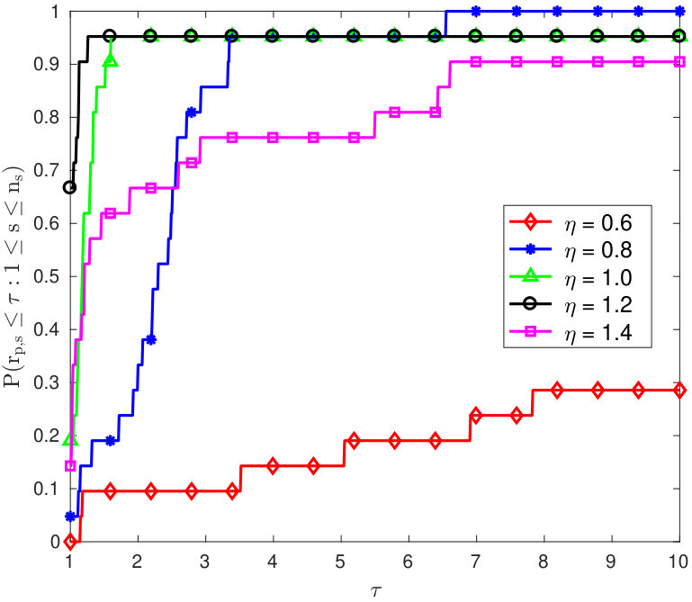 Figure 1
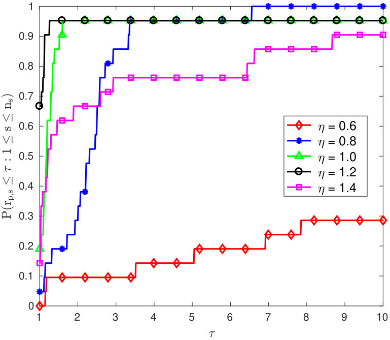 Figure 1
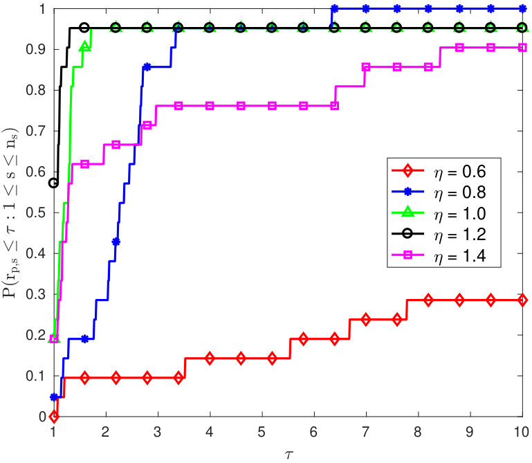 Figure 1
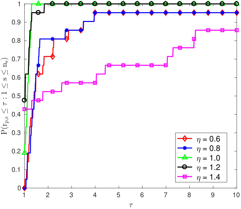 Figure 1
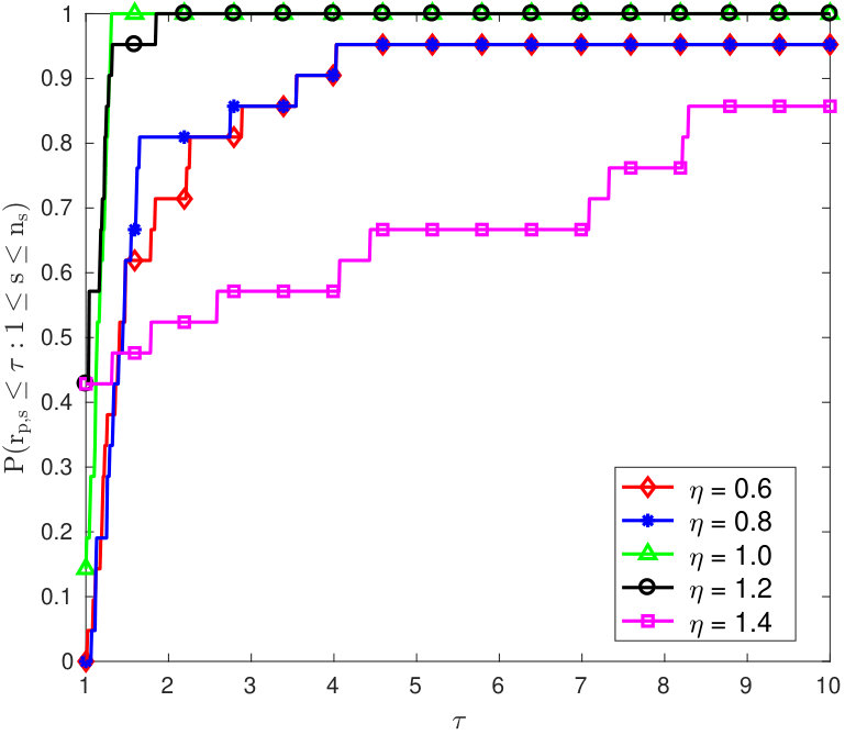 Figure 1
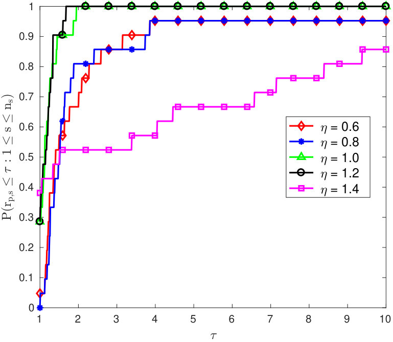 Figure 1
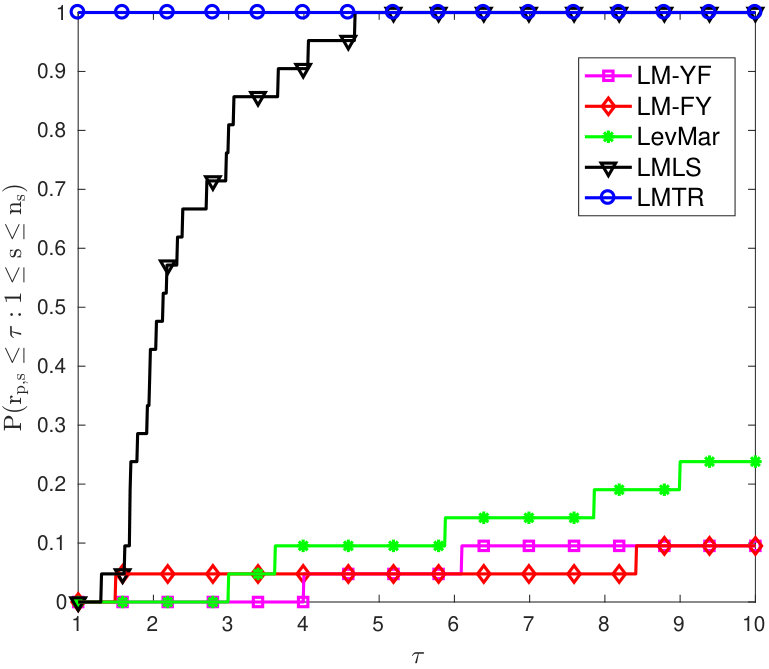 Figure 2
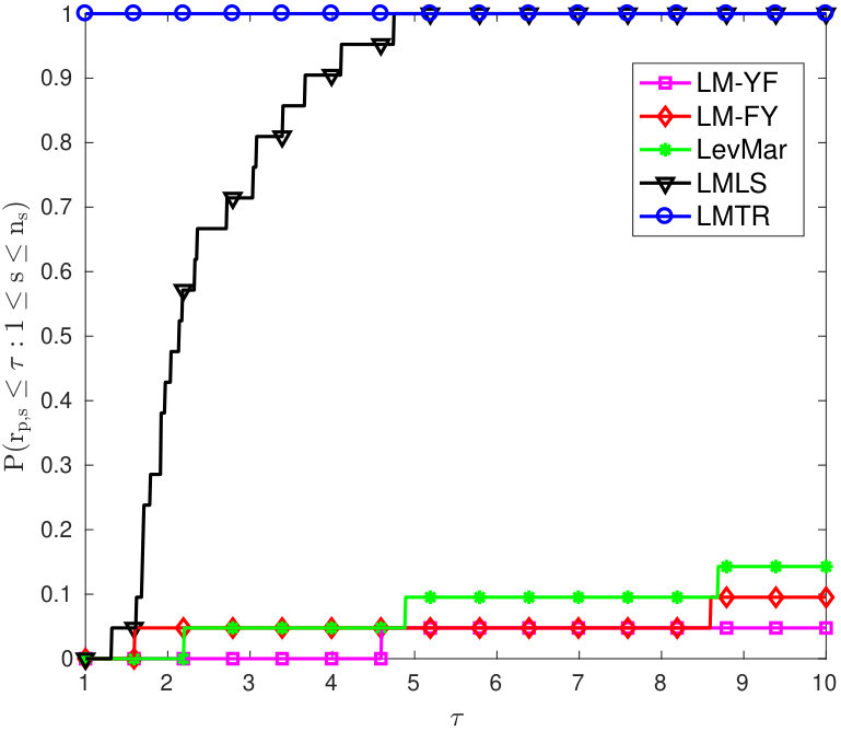 Figure 2
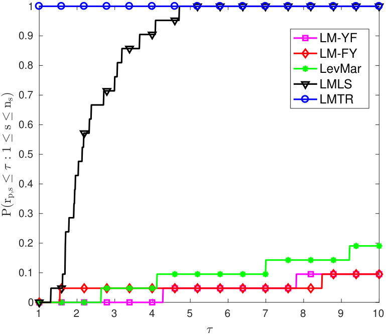 Figure 2
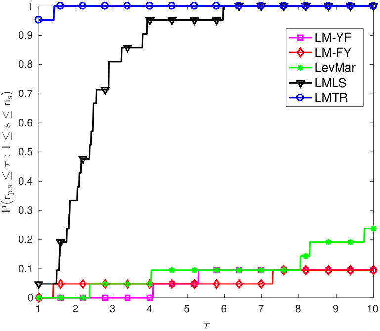 Figure 2
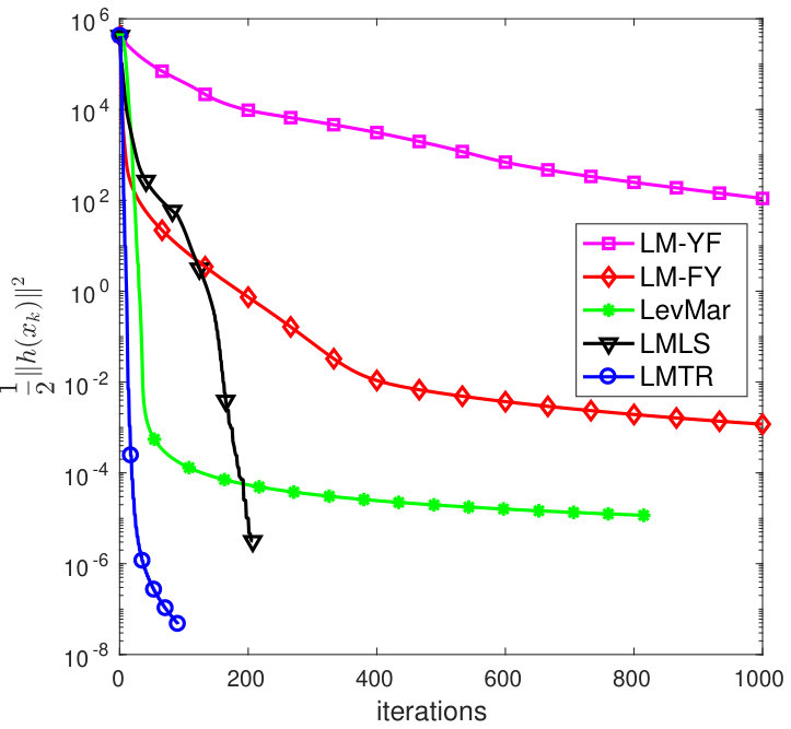 Figure 3
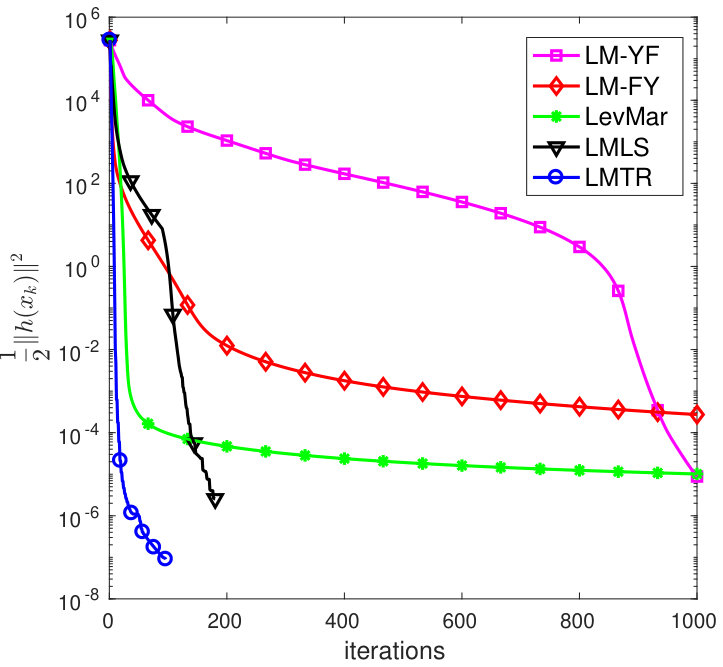 Figure 3
| Model | Model | ||||||
|---|---|---|---|---|---|---|---|
| 1. Ecoli_core | 72 | 73 | 61 | 12. iMB745 | 525 | 598 | 490 |
| 2. iAF692 | 462 | 493 | 430 | 13. iNJ661 | 651 | 764 | 604 |
| 3. iAF1260 | 1520 | 1931 | 1456 | 14. iRsp1095 | 966 | 1042 | 921 |
| 4. iBsu1103 | 993 | 1167 | 956 | 15. iSB619 | 462 | 508 | 435 |
| 5. iCB925 | 415 | 558 | 386 | 16. iTH366 | 583 | 606 | 529 |
| 6. iIT341 | 424 | 428 | 392 | 17. iTZ479_v2 | 435 | 476 | 415 |
| 7. iJN678 | 641 | 669 | 589 | 18. iYL1228 | 1350 | 1695 | 1280 |
| 8. iJN746 | 727 | 795 | 700 | 19. L_lactis_MG1363 | 483 | 491 | 429 |
| 9. iJO1366 | 1654 | 2102 | 1582 | 20. Sc_thermophilis_rBioNet | 348 | 365 | 320 |
| 10. iJP815 | 524 | 595 | 501 | 21. T_Maritima | 434 | 470 | 414 |
| 11. iJR904 | 597 | 757 | 564 |
Peer Reviews
No public reviews on file for this paper yet. If you reviewed it on a platform where reviews are public (OpenReview, ICLR, NeurIPS, ICML), you can paste yours below so the community can read it here.
Videos
No videos yet. Explain this paper in a talk, walkthrough, or lecture? Add one.
Finding Zeros of Hölder Metrically Subregular Mappings via Globally Convergent Levenberg–Marquardt Methods
Masoud Ahookhosh, Ronan M.T. Fleming, Phan T. Vuong Luxembourg Center for Systems Biomedicine, University of Luxembourg, Campus Belval, 4362 Esch-sur-Alzette, Luxembourg. Present address: KU Leuven, Stadius Centre for Dynamical Systems, Signal Processing and Data Analytics, Kasteelpark Arenberg 10, 3001 Leuven. E-mail: [email protected] Luxembourg Center for Systems Biomedicine, University of Luxembourg, Campus Belval, 4362 Esch-sur-Alzette, Luxembourg. Present address: Leiden University, Leiden Academic Centre for Drug Research, Einsteinweg 55, Leiden, NL 2333 CC, Netherlands. E-mail: [email protected]Luxembourg Center for Systems Biomedicine, University of Luxembourg, Campus Belval, 4362 Esch-sur-Alzette, Luxembourg. Present address: Institute of Statistics and Mathematical Methods in Economics, Vienna University of Technology, Austria. E-mail: [email protected]
Abstract
We present two globally convergent Levenberg–Marquardt methods for finding zeros of Hölder metrically subregular mappings that may have non-isolated zeros. The first method unifies the Levenberg–Marquardt direction and an Armijo-type line search, while the second incorporates this direction with a nonmonotone trust-region technique. For both methods, we prove the global convergence to a first-order stationary point of the associated merit function. Furthermore, the worst-case global complexity of these methods are provided, indicating that an approximate stationary point can be computed in at most function and gradient evaluations, for an accuracy parameter . We also study the conditions for the proposed methods to converge to a zero of the associated mappings. Computing a moiety conserved steady state for biochemical reaction networks can be cast as the problem of finding a zero of a Hölder metrically subregular mapping. We report encouraging numerical results for finding a zero of such mappings derived from real-world biological data, which supports our theoretical foundations.
Keywords: Nonlinear equation, Hölder metric subregularity, Non-isolated solutions, Levenberg-Marquardt methods, Global convergence, Worst-case global complexity, Biochemical reaction network kinetics.
AMS subject classifications: 90C26, 68Q25, 65K05
1 Introduction
We consider the problem of finding zeros of the nonlinear mapping , i.e.,
[TABLE]
where is continuously differentiable and satisfies the Hölder metric subregularity (see bellow). The set of zeros of such mappings is denoted by , which is assumed to be nonempty.
A classical approach for finding a solution of (1) is to search for a minimiser of the nonlinear least-squares problem
[TABLE]
where denotes the Euclidean norm. In order to guarantee the quadratic or superlinear convergence of many Newton-type schemes for solving (2), the existence of some constant satisfying
[TABLE]
is assumed, where stands for the closed ball centered at with radius , cf. [27, 48]. Such an inequality is referred as an error bound (Lipschitzian error bound or metric regularity) condition. The notion of error bound has been very popular during the last few decades to study the local convergence of optimisation methodologies; however, there are many important mappings where (3) is not satisfied , see, e.g., [4, 34]. This motivated the authors of [4] to propose a weaker condition so-called the Hölder metric subregularity (Hölderian error bound), i.e.,
[TABLE]
for and . There are many mappings satisfying this condition, see, e.g., [4, 34] and references therein. See also Section 5 for a real-world nonlinear system satisfying (4), but not (3).
The Levenberg–Marquardt method is a standard technique used to solve (1), where, in the current point and for a positive parameter , the convex subproblem
[TABLE]
is solved to compute a direction in which is the gradient of at . This requires finding the unique solution of the linear system
[TABLE]
where denotes the identity matrix. Then, the next iteration is be generated by and this scheme is continued until a stationary point of (2) is found, which may correspond to a zero , when certain conditions are satisfied.
The choice of the parameter has substantial impacts on the global convergence, the local convergence rate, and the computational efficiency of Levenberg–Marquardt methods, cf. [4, 31, 38, 47, 48]. Hence, several ways to specify and to adapt this parameter have been proposed; see, e.g., [18, 19, 48]. A recently proposed Levenberg–Marquardt method by the authors [4] suggests an adaptive parameter based on the order of the Hölder metric subregularity (4), i.e.,
[TABLE]
where , and with . In [4], this Levenberg–Marquardt method, with adaptive regularisation (LM-AR), was presented and its local convergence was studied for Hölder metrically subregular mappings.
If one assumes that the starting point is close enough to a solution of (2), then the Levenberg–Marquardt method is known to be quadratically convergent if is nonsingular, in which case it is clearly convergent to a solution to (1). In fact, the nonsingularity assumption implies that the solution of the minimisation problem (2) must be locally unique; see [10, 28, 48]. However, assuming local uniqueness of the solution might be restrictive for many applications since the underlying mappings might have non-isolated zeros. Therefore, much attention has been devoted to the study of local convergence of the Levenberg–Marquardt method under local error bounds, which enables the solution of mappings with non-isolated zeros; see, e.g., [10, 18, 19, 48]. In particular, the local convergence of the Levenberg–Marquardt method was studied in [4] under the Hölder metric subregularity condition (4).
As is the case in many applications, one cannot provide a sufficiently close starting point to a solution , and therefore the convergence of the Levenberg–Marquardt method is not guaranteed, which decreases the chance of practical applicability. To overcome this shortcoming, two globalisation techniques have been proposed to be combined with the Levenberg–Marquardt direction, namely, line search and trust-region; see, e.g., [3, 31, 30, 44]. Generally, a line search method finds a descent direction , specifies a step-size , generates the new iteration , and repeats this scheme until a stopping criterion holds. The step-size is usually determined by an inexact line search such as Armijo, Wolfe, or Goldstein backtracking schemes; see [14, 43]. In particular, the Armijo line search usually finds using a backtracking procedure, which ends up with a step-size satisfying
[TABLE]
where . In order to provide an outline for trust-region methods, let us define, firstly, the quadratic function with
[TABLE]
Then, a Levenberg–Marquardt trust-region method solves the quadratic subproblem (5) to find a direction , computes the ratio of the actual reduction to the predicted reduction
[TABLE]
and updates the parameter using . For line search and trust-region methods, the global convergence to a first-order stationary point of can be guaranteed, which results to a monotone sequence of function values, i.e., .
Regardless of the fact that the monotonicity seems natural for the minimisation goal, it has some drawbacks. We address two of them here: (i) the monotone method may lose its efficiency if iterations are trapped at the bottom of a curved narrow valley, where the monotonicity forces the iterations to trace the valley floor (causing very short steps or even an undesired zigzagging); (ii) the Armijo-type line search can break down for very small step-sizes because of rounding errors, when . In this case, the point may still be far from a stationary point of ; however, the Armijo rule cannot be satisfied due to indistinguishability of from in floating-point arithmetic. To overcome such limitations, the seminal article by Grippo et al. [22] addressed a variant of the Armijo rule (8) by substituting with , where and , for some nonnegative integer constant for all . This does not guarantee the monotonicity condition and therefore called nonmonotone. Nonmonotonicity has also been studied for trust-region methods by replacing with a nonmonotone term; cf. [1]. On the basis of many studies in this area, nonmonotone methods have been recognised to be globally convergent and computationally efficient, even for highly nonlinear problems; see [1, 5] and references therein.
1.1 Motivation and contribution
Our analysis was motivated by the problem of finding moiety conserved steady states of deterministic equations representing the dynamical evolution of molecular species abundance in biochemical reaction networks. This problem can be considered as an application of finding zeros of a mapping , that may not satisfy the local error bound (3). It was previously established [4] that this mapping is Hölder metrically subregular and that the merit function is real analytic using standard biochemical assumptions; cf. [7]. Applying a novel Levenberg–Marquardt algorithm with adaptive regularisation (LM-AR), to this problem, we proved local convergence to a zero of for all such networks if the sufficiently closeness of a starting point to can be assumed [4]. However, providing a starting point close enough to remains as a limitation in practice, as is the case for all local optimisation methods; see, e.g., [14, 16].
The global convergence and complexity of iterative methods has been the subject of intense debate within the nonlinear optimisation community over the last few decades. While the global convergence guarantees the convergence of the iteration sequence generated by a method for any given starting point , the worst-case complexity provides an upper bound on the number iterations or function evaluations needed to reach a stationary point of the underlying objective function. These two factors are more important if the convexity or structured nonconvexity of the objective function is assumed; see, e.g., [8, 11, 39, 40, 41, 49]. In the particular case of solving nonlinear least-squares problems by Levenberg-Marquardt methods, there are less results about their global convergence and complexity, compared with the volume of literature concerning Newton-type methods; cf. [45, 46]. This motivates our aim to study the global convergence properties and complexity of two Levenberg-Marquardt methods using line search and trust-region techniques.
We analyse the global convergence, and investigate the complexity of, two Levenberg–Marquardt methods using line search scheme and trust-region globalisation techniques. For the first method, we use defined in (7), solve the linear system (6) to specify , and combine this direction with a nonmonotone Armijo-type line search. We also propose a modified version of the Levenberg–Marquardt parameter (7), which is lower bounded, and combines the associated direction with a trust-region technique to adapt the Levenberg–Marquardt parameter. A global convergence analysis is provided for both methods. Moreover, we demonstrate that, for both methods, a first-order stationary point is attained after at most iterations or function evaluations. We also illustrate some special mappings where the proposed methods are convergent to a solution to the nonlinear system (1). Finally, we demonstrate that the application of these two methods mappings derived from real-world biochemical reaction networks, from a diverse set of biological species, shows encouraging numerical results in practice. To the best of our knowledge, these two Levenberg–Marquardt methods are the first methods, globally convergent to a stationary point, for finding zeros of the mapping arising in the study of biological networks. All algorithms are made available within the COBRA Toolbox v.03 [25], an open source software package for modelling biochemical reaction networks.
This paper has five sections, besides this introductory section. Section 2 describes a globally convergent Levenberg–Marquardt line search method. Section 3 addresses a globally convergent Levenberg–Marquardt trust-region method, where in both sections the global convergence and complexity of these methods are analysed. In Section 4, finding a zero of some specific mappings with the proposed methods is discussed. Section 5 reports encouraging numerical results for a mapping appearing in biochemical reaction networks. Finally, conclusions and area for further research are identified in Section 6.
2 Levenberg–Marquardt line search method
For the sake of simplicity, we define . If is not a stationary point of , from positive definiteness of , we obtain
[TABLE]
which guarantees the descent property of at . This motivates us to develop a globally convergent Levenberg–Marquardt method using (7). More precisely, we shall combine the Levenberg–Marquardt direction with a nonmonotone Armijo-type line search using the nonmonotone term
[TABLE]
A combination of the direction (given by solving (6) using the parameter (7)) with a nonmonotone Armijo-type line search using (12) leads to Algorithm 1.
In order to prove the global convergence of the sequence generated by LMLS to a stationary point of , we assume that the next assumptions hold:
(A1)
The mapping is continuously differentiable and Hölder metrically subregular of order at ; i.e., there exist some constants and such that (4) holds;
(A2)
The lower level set is bounded;
(A3)
is Lipschitz continuous, i.e.,
[TABLE]
In the subsequent proposition, we first derive a lower bound for the step-size and give a bound on the total number of function evaluations needed until the line search (Line 5 of LMLS) is satisfied.
Proposition 2.1**.**
Let be an infinite sequence generated by LMLS. Then,
(i)
;
(ii)
if LMLS does not terminate at , then
[TABLE]
with
[TABLE]
for . Moreover, the inner loop of LMLS is terminated in a finite number of steps, denoted by , which satisfies
[TABLE]
?proofname?
.
We prove Assertions (i) and (ii) by induction at the same time. Let us assume . Since , by the traditional results about the monotone Armijo line search, we have . This implies that . The proof of Assertion (ii) is similar to , i.e., we therefore omit it.
We now assume Assertions (i) and (ii) hold for and prove them for . Since satisfies the line search and , similar to Lemma 2.3 in [2], we can show . This and
[TABLE]
imply and
[TABLE]
Therefore,
[TABLE]
leading to , i.e., Assertion (i) holds for .
From (A1) and , there exists some constant such that
[TABLE]
which implies
[TABLE]
leading to
[TABLE]
From the definition of , we obtain
[TABLE]
Since LMLS does not stop at , it holds and , which imply
[TABLE]
Let us consider a constant , i.e.,
[TABLE]
We first derive a lower bound on the step-size . By (20), (18) and (21), we get
[TABLE]
Therefore, for all , we have
[TABLE]
Further, for all and , (A3) and (22) yield
[TABLE]
It follows from (18) that
[TABLE]
By this inequality, the Taylor expansion of around , and the Cauchy–Schwarz inequality, for any , we come to
[TABLE]
This inequality, (18), (23), (24), and (A3) suggest
[TABLE]
From (16), we come to
[TABLE]
For , we have
[TABLE]
which yields
[TABLE]
For , the Armijo-type line search (Line 5 of LMLS) does not hold, i.e.,
[TABLE]
This and the inequality (27) lead to
[TABLE]
Substituting , we have thanks to (20) and (19) that
[TABLE]
It follows from (28) and (21) that (13) is valid. Using and (13), we end up to
[TABLE]
which proves (14). ∎
The first main result of this section demonstrates some properties of the sequence and shows that any accumulation point of the sequence generated by LMLS is either a solution of (1) or a stationary point of .
Theorem 2.2**.**
Let be an infinite sequence generated by LMLS. Then, for all , the following assertions hold:
(i)
* is convergent and*
[TABLE]
(ii)
;
(iii)
LMLS either stops at finite number of iterations, satisfying or , or generates an infinite sequence such that any accumulation point of this sequence is a stationary point of the merit function , i.e.,
[TABLE]
?proofname?.
From (15), we have . This, Proposition 2.1 (i) and (A2) imply that is convergent. Further, since , with , we have . Taking limits from both sides of when goes to infinity, we deduce (29).
It follows from (19) and the definition of that
[TABLE]
By the definition of , (17), and (18), we get
[TABLE]
for all . This and (31) yield
[TABLE]
that is, Assertion (i) holds with .
Let us now prove the assertion (iii). If the algorithm stops in a finite number of iterations by either or , the result is valid. Let us assume that the algorithm generates an infinite sequence . For a fixed iteration , the stopping criteria of LMLS do not hold, i.e., and . Therefore, from (21), we have
[TABLE]
It can be deduced from Line 5 of LMLS and Assertion (ii) that
[TABLE]
This and the assertion (ii) yield
[TABLE]
i.e., any accumulation point of is a stationary point of . ∎
We continue the analysis of LMLS by providing the worst-case global and evaluation complexities of LMLS, which are upper bounds on the number of iterations and merit function evaluations required to get an approximate stationary point of satisfying , for the accuracy parameter , respectively. Let us denote by and the total number of iterations and merit function evaluations of LMLS required to find and an -stationary point of (2) .
Theorem 2.3**.**
Let be the sequence generated by LMLS and (A2) and (A3) hold. Then,
(i)
the total number of iterations to guarantee is bounded above and
[TABLE]
with ;
(ii)
the total number of function evaluations to guarantee is bounded above and
[TABLE]
?proofname?.
To prove Assertion (i), we define
[TABLE]
which suggests
[TABLE]
Let us assume by contradiction that , which means that the algorithm does not stop in iterations. From Line 5 of LMLS, (15), and Theorem 2.2 (ii), we obtain
[TABLE]
leading to
[TABLE]
which contradicts to (36). Therefore, (34) is valid.
Considering the bound on the number of merit function evaluations in step (, given in Proposition 2.1), the following upper bound on the total number of merit function evaluations can be provided by
[TABLE]
giving the results. ∎
Theorem 2.3 implies that the worst-case global and evaluation complexities of LMLS to attain the approximate stationary point of are of the order , which is the same as the gradient method; see, e.g., [39]. However, in practice Levenberg-Marquardt methods usually performs much better than the gradient method.
Let us compute here the second derivative of at , i.e.,
[TABLE]
where . Three types of the problem (1) are recognised with respect to the magnitude of : (i) if , the problem is called zero residual; (ii) if is small, the problem is called small residual; and if is large, the problem is called large residual; see, e.g., [16]. Under the nonsingularity assumption of at the limit point of and using (37), we investigate the superlinear convergence of generated by LMLS for zero residual problems, which is the same as the convergence rate given for quasi-Newton methods; see [15].
Theorem 2.4**.**
Let be twice continuously differentiable on , and be the sequence generated by LMLS and (A1)-(A3) hold. If converges to and has full rank, then
[TABLE]
there exists such that for all , and converges to superlinearly.
?proofname?.
Since has full rank, (30) implies . This and (37) yield that is positive definite. Hence, leads to
[TABLE]
From (37), we obtain
[TABLE]
which implies
[TABLE]
Since is twice continuously differentiable in the compact set , () is bounded. This, the last inequality, and (39) give
[TABLE]
giving (38).
From Theorem 6.4 in [15] and (38), we have that (8) is valid with , for all sufficiently large. Therefore, the superlinear convergence of follows from Theorem 3.1 in [15]. ∎
3 Levenberg–Marquardt trust-region method
Trust-region methods are known to be effective for nonconvex optimisation problems (see [14]). Therefore, this section concerns with the development of a globally convergent Levenberg–Marquardt method using a trust-region technique and the investigation on its convergence analysis and complexity.
Let us start with some details of a trust-region globalisation technique that will be coupled with the Levenberg–Marquardt direction. We first draw your attention to some literature, e.g., [1, 3] and references therein, about the efficiency of nonmonotone trust-region methods compared to monotone ones for either optimisation or nonlinear systems. This motivates us to develop a nonmonotone Levenberg–Marquardt trust-region method for solving systems of nonlinear equations. To do so, we take advantage of the quadratic function (9) and define the ratio
[TABLE]
where the nonmonotone term defined by (12). In this ratio, the nominator is called nonmonotone reduction and the denominator is called the predicted reduction. Further, let us introduce a new Levenberg–Marquardt parameter that is a modified version of (7), i.e.,
[TABLE]
where is given by (7) with , , , with , and is updated by
[TABLE]
in which and are some constants. A simple comparison between (7) and (41) indicates that is lower bounded and helps to have a better control on the Levenberg–Marquardt parameter, which shows its effect on numerical performance of the method (see Section 5 for more details).
In our Levenberg–Marquardt trust-region method, we first determine (41), specify the direction by solving the linear system (6), and compute the ratio (40). If , the trial point is accepted, i.e., ; otherwise, the parameter should be increased by setting . In the case that , the parameter is decreased by setting . The final step will be the evaluation of stopping criteria, which here is either or . We summarise this scheme in Algorithm 2.
In LMTR, the loop starts from Line 5 to Line 7 is called the inner loop and the loop starts from Line 3 to Line 14 is called the outer loop.
The subsequent proposition points out that the inner loop of LMTR is terminated after a finite number of steps and provides upper bounds for and .
Proposition 3.1**.**
Let be an infinite sequence generated by LMTR and (A1)-(A3) holds. Then,
(i)
;
(ii)
;
(iii)
the inner loop is terminated in a finite number of steps. Moreover, if LMTR does not terminate at , then
[TABLE]
with
[TABLE]
and
[TABLE]
?proofname?.
By the definition of in (9) and (19), we get
[TABLE]
giving Assertion (i).
It follows from (9) that
[TABLE]
proving Assertion (ii).
For the first part of the assertion (iii), we show that the inner loop is terminated after a finite number of steps. From Assertion (i) and (20), we obtain
[TABLE]
By (A3) and (20), for , we get
[TABLE]
By the Taylor expansion of around , we come to
[TABLE]
From this, (23), and (47), it consequently holds
[TABLE]
Since , we have . This and
[TABLE]
imply and , leading to , i.e.,
[TABLE]
It can be deduced from this and (49) that
[TABLE]
where , , and . For sufficiently large , we have . This, (10), and (46) yield
[TABLE]
It can be deduced from this and that , for sufficiently large , proving the first part of Assertion (iii).
In the second part of Assertion (iii), we provide upper bounds for and . Let us denote by the solution of the system (6) corresponding to the parameter and set . By (20) and (18), we get
[TABLE]
It follows from this and the triangle inequality that
[TABLE]
For all , (A3) and (53) imply
[TABLE]
From (18), (2), (48), and (11), we obtain
[TABLE]
Following and , it can be deduced
[TABLE]
It follows from (45) and the definition that and
[TABLE]
Combining this inequality with that in (56) suggest
[TABLE]
leading to
[TABLE]
giving (42). Since , taking the logarithm from both sides of
[TABLE]
implies (43), completing the proof. ∎
We now draw your attention to the global convergence of the sequence generated by LMTR to a first-order stationary point of satisfying . Let us first recall the following result for local convergence of the Levenberg–Marquardt method given in [4].
Theorem 3.2**.**
Let be the sequence generated by LMTR and (A1)-(A3) hold. Then, is convergent and
[TABLE]
Further, the algorithm either stops at finite number of iterations, satisfying or , or generates an infinite sequence such that any accumulation point of this sequence is a stationary point of the merit function , i.e.,
[TABLE]
?proofname?.
From (50) and (51), we have and . Hence, the sequence is decreasing and bounded below, i.e., it is convergent. From , with , we obtain . Taking limits when goes to infinity from gives (57).
If the algorithm stops in a finite number of iterations by either or , the result is valid. If the algorithm generates the infinite sequence , Proposition 3.1 (i) yields
[TABLE]
From this and (57), we obtain
[TABLE]
i.e., any accumulation point of is a stationary point of . ∎
Let us continue this section by providing global and evaluation complexities of the sequence generated by LMTR using the results presented in Proposition 3.1.
Theorem 3.3**.**
Let be the sequence generated by LMTR and (A1)-(A3) hold. Then,
(i)
the total number of iterations to guarantee is bounded above by
[TABLE]
where ;
(ii)
the total number of function evaluations to guarantee is bounded above by
[TABLE]
?proofname?.
To prove Assertion (i), we first define
[TABLE]
which is equivalent to
[TABLE]
Let us assume by contradiction that , which means that LMTR does not stop in iterations. For a successful iteration of LMTR, it follows from (15) and Proposition 3.1 (i) that
[TABLE]
leading to
[TABLE]
which contradicts to (61), proving Assertion (i).
[TABLE]
giving (60). ∎
We conclude this section by providing the local convergence rate of LMTR if the corresponding sequence is convergent to a solution of (1) under the Lojasiewicz gradient inequality (see [35, 36]). To this end, the presence of the subsequent two lemmas are necessary in our local analysis of LMTR.
Lemma 3.4**.**
[7, Lemma 1]** Let be a sequence in and let be some nonnegative constants. Suppose that and that the sequence satisfies
[TABLE]
for all sufficiently large. Then
- (i)
if , the sequence converges to [math] in a finite number of steps; 2. (ii)
if , the sequence converges linearly to [math] with rate ; 3. (iii)
if , there exists such that, for all sufficiently large,
[TABLE]
Lemma 3.5**.**
[29, Theorem 2.5 and Lemma 2.3]** The sequence generated by LMTR with satisfies
[TABLE]
and
[TABLE]
Let us describe now the Łojasiewicz gradient inequality in the following definition.
Definition 3.6**.**
Let be a function defined on an open set , and assume that the set of zeros is nonempty. The function is said to satisfy the Łojasiewicz gradient inequality if for any critical point , there exist constants and such that
[TABLE]
This inequality is valid for a large class of functions such as analytic, subanalytic, and semialgebraic functions, cf. [35, 36, 33]. See Section 5 for a mapping with a real analytic merit function, where finding zeros of this mapping is the main motivation of this study. Here, we further assume that
(A4)
the merit function satisfies the Łojasiewicz gradient inequality (64).
The next theorem is the third main result of this section, which provides the convergence of the sequences and to [math] if an accumulation point of is a solution of the nonlinear system (1).
Theorem 3.7**.**
Suppose that (A4) holds and assume that the sequence generated by LMTR is convergent to a solution of the nonlinear system (1). Then,
- (i)
for sufficiently large , it holds ; 2. (ii)
there exist constants , , and such that, for ,
[TABLE] 3. (iii)
if , the sequences and converge to [math] in a finite number of steps; 4. (iv)
if , the sequences and converge linearly to [math]; 5. (v)
if , there exist some positive constants and such that, for all large ,
[TABLE]
?proofname?.
Since is an accumulation point of and a solution of the nonlinear system (1), it can be deduced
[TABLE]
From this, Proposition 3.1 (i), Proposition 2.1 (ii), (49), , and (65), we obtain
[TABLE]
which implies that there exists a such that . Hence, for all , it follows from that
[TABLE]
which means that with that justifies Assertion (i).
We divide the proof of Assertion (ii) into three parts. First, we will provide the values of and . Let us set and such that (64) holds and let . By the definition of , (A2), and (42), we get
[TABLE]
By making smaller if needed, we can guarantee
[TABLE]
Lipschitz continuity of and , for all , lead to
[TABLE]
We now define
[TABLE]
From and , we obtain .
For , let us choose any . Lemma 3.5 and imply, for all ,
[TABLE]
Next, let us show by induction that, for ,
[TABLE]
It follows from and (67) that
[TABLE]
leading to
[TABLE]
Then, from (69), one can deduce
[TABLE]
From the convexity of the function with , we come to
[TABLE]
This and (71) suggest
[TABLE]
It follows from and (66) that . Hence, by the Łojasiewicz gradient inequality (64), we get
[TABLE]
[TABLE]
which, proves the second assertion in (70) for . Then, we have
[TABLE]
implying . Now, let us assume that (70) holds for all . From and (67), it can be deduced
[TABLE]
leading to
[TABLE]
It follows from this and (69) that
[TABLE]
A combination of this inequality and (72) leads to
[TABLE]
Further, from , (64), and (66), we obtain
[TABLE]
By the latter inequality and (75), we come to
[TABLE]
proving the second assertion in (70) for . Then, it follows from (68) that
[TABLE]
Hence, the first assertion in (70) is valid for .
Finally, we are in a position to show that Assertions (ii) is true. As shown in (70), for all . This and (66), implies that for all . Hence, for , we have
[TABLE]
Then, by (74), we get
[TABLE]
From this and (64), it can be deduced
[TABLE]
which implies that converges to [math]. This ans the Hölder metric subregularity validate the statement of the assertion (ii).
Applying Lemma 3.4 with , and , we have that the convergence rate are dependent to as claimed in Assertions (iii)-(v). Therefore, the Hölder metric subregularity of implies that converges to [math] with the rate given in (iii)-(v). ∎
4 Convergence to a solution of nonlinear systems
Let us emphasis that the algorithms LMLS and LMTR only guarantee the convergence of the sequence to a stationary point of the merit function , which can be a local non-global minimiser of (2), i.e.,
[TABLE]
Therefore, the remainder of this section concerns with considering more restrictions on the mapping such that the global convergence of to a solution of (1) is guaranteed.
The next theorem extracts some classical results for cases that is nonsingular, which implies that is a solution of (1). Moreover, the worst-case global and evaluation complexities to attain solution of (1) are provided under the nonsingularity of for all . Under the assumption that all accumulation points of are solutions of (1) and is nonsingular for the accumulation point , it is proved that the whole sequence converges to the isolated solution of (1).
Theorem 4.1**.**
Let be the sequence generated by LMLS or LMTR and (A1)-(A3) hold. Then
(i)
if is nonsingular at any accumulation point of , then is a solution of the nonlinear system (1).
(ii)
if the matrix is nonsingular for all , i.e., there exists such that , then, for LMLS,
[TABLE]
and
[TABLE]
and, for LMTR,
[TABLE]
and
[TABLE]
(iii)
*if all accumulation points of are solutions of the nonlinear system (1), *is an accumulation point of such that is nonsingular, and
[TABLE]
then converges to .
?proofname?.
For any accumulation point of , it follows from Theorem 3.2 that . This, along with the nonsingularity of , implies Assertion (i).
To prove Assertion (ii), we note that
[TABLE]
i.e., . This and Proposition 2.3 (i)-(ii) give (76) and (77), respectively. Similarly, (78) and (79) follow from this inequality and Proposition 3.3 (i)-(ii).
In order to prove Assertion (iii), let us assume that all accumulation points of are solutions of (1), is an accumulation point such that is nonsingular, and (80) holds. From the inverse function theorem and the nonsingularity of , there exists a neighborhood around 0 such that is invertible. Therefore, there exists a neighborhood for such that
[TABLE]
implying
[TABLE]
Since is an accumulation point of , contains an infinite number of iteration points of . It remains to show that there exists such that , for all . Hence, for an arbitrary , the set involves only a finite number of iterations of , i.e., there exists such that
[TABLE]
It follows from (80) that there exists such that
[TABLE]
Let us set leading to
[TABLE]
giving the result. ∎
The mapping is called strictly monotone on if
[TABLE]
In addition, the mapping is called strictly duplomonotone with constant if
[TABLE]
whenever ; see [6, 44]. In the next result, we will show that if the mapping or is strictly monotone (duplomonotone), then the sequence generated by LMLS converges to the unique solution of the nonlinear system (1).
Theorem 4.2**.**
Let be the sequence generated by LMLS or LMTR and (A1)-(A3) hold.
(i)
If the mapping or is strictly monotone, then converges to the unique solution of the nonlinear system (1).
(ii)
If the mapping or is strictly duplomonotone, then converges to a solution of the nonlinear system (1).
?proofname?.
In order to prove Assertion (i), let or be strictly monotone and be an accumulation point of . If is strictly monotone, for the points and with and , we can deduce
[TABLE]
If is strictly monotone, then
[TABLE]
By setting and in the last two inequalities, we get
[TABLE]
To prove Assertion (ii), let be strictly duplomonotone, which leads to
[TABLE]
If is strictly duplomonotone, then
[TABLE]
The result follows from the last two inequalities at , (30), and (58). ∎
Note that the strict monotonicity of does not implies the positive definiteness of . Therefore the results of Theorem 4.2 (i) is not a trivial consequence of Theorem 4.1 (i).
5 Application to biochemical reaction networks
In this section, we use the following notation: , , and . Let us consider a biochemical reaction network with molecular species and reversible elementary reactions111An elementary reaction is a chemical reaction for which no intermediate molecular species need to be postulated in order to describe the chemical reaction on a molecular scale.. We define forward and * reverse stoichiometric matrices*, , respectively, where denotes the stoichiometry222Reaction stoichiometry is a quantitative relationship between the relative quantities of molecular species involved in a single chemical reaction. of the molecular species in the forward reaction and denotes the stoichiometry of the molecular species in the reverse reaction. We assume that every reaction conserves mass, i.e., there exists at least a positive vector such that ; cf. [21]. The matrix represents net reaction stoichiometry and may be viewed as an incidence matrix of a directed hypergraph; see [32]. In practice, there are less molecular species than net reactions (). We assume the cardinality of each row of and is at least one, and the cardinality of each column of is at least two. The matrices and are sparse and the sparsity pattern depends on the particular biochemical reaction network being modeled. It is here assumed that , which is a requirement for kinetic consistency; cf. [20].
Let be a vector of molecular species concentrations. For nonnegative elementary kinetic parameters , elementary reaction kinetics for forward and reverse elementary reaction rates as and , respectively, where and denote the respective componentwise functions; see, e.g., [7, 20]. Then, the system of differential equations
[TABLE]
shows the deterministic dynamical equation for time evolution of molecular species concentration. A vector is called a steady state if and only if . Hence, is a steady state of the biochemical system if and only if
[TABLE]
where stands for the null space of . The set of steady states will be unchanged if is replaced by a matrix with the same kernel. Suppose that is the submatrix of whose rows are linearly independent, then If one replaces by and transforms (5) into logarithmic scale, by letting , , then the right-hand side of (5) can be translated to
[TABLE]
where stands for the horizontal concatenation operator.
Let be a basis for the left nullspace of , i.e., , where and . The system satisfies moiety conservation if for any initial concentration , it holds
[TABLE]
where It is possible to compute such that each corresponds to a structurally identifiable conserved moiety in a biochemical reaction network; cf. [24]. Therefore, finding the moiety conserved steady state of a biochemical reaction network is equivalent to finding a zero of the mapping
[TABLE]
It was shown by the authors in Section 4.1 of [4] that the merit function satisfies Łojasiewicz gradient inequality (with an exponent ) and the mapping is Hölder metrically subregular at , i.e., the assumption (A1) holds.
5.1 Computational results
We find zeros of the mapping (83) with a set of real-world biological data using LMLS and LMTR. In details, we compare the performance of LMLS and LMTR with some state-of-the-art algorithms on a set of 21 biochemical reaction networks given in Table 1. In Section 4.2 of [4], it is computationally shown that is rank-deficient or ill-conditioned at zeros of the mapping (83) for these biological models. This clearly justifies the reason of unsuccessful performance of many existing algorithms (e.g., gradient descent, Gauss-Newton, and trust-region methods) and vindicates the development of the two adaptive Levenberg-Mardquart methods (LMLS and LMTR) for such difficult problems.
All codes are written in MATLAB and runs are performed on a Dell Precision Tower 7000 Series 7810 (Dual Intel Xeon Processor E5-2620 v4 with 32 GB RAM). We compare LMLS and LMTR with
LM-YF: a Levenberg–Marquard line search method with , given by Yamashita and Fukushima [48];
LM-FY: a Levenberg–Marquardline search method with , given by Fan and Yuan [18];
LevMar: a Levenberg–Marquard trust-region method with , given by Ipsen et al. [26].
The codes of LMLS and LMTR are publicly available as a part of the COBRA Toolbox v3.0 [25]. Users can pass the solver name to the parameter structure of the MATLAB function optimizeVKmodels.m. For both LMLS and LMTR, on the basis of our experiments with the mapping (83), we set and
[TABLE]
implying . We here use the starting point and consider the stopping criterion
[TABLE]
cf. [9]. We stop the algorithms if either (85) holds or the maximum number of iterations (say 10,000 for tuning and 100,000 for the comparison) is reached. While LMLS uses the parameters
[TABLE]
LMTR employs the parameters
[TABLE]
In our comparison, , and denote the total number of iterations, the total number of function evaluations, and the running time, respectively. To illustrate the results, we used the Dolan and Moré performance profile [17] with the performance measures and . In this procedure, the performance of each algorithm is measured by the ratio of its computational outcome versus the best numerical outcome of all algorithms. This performance profile offers a tool to statistically compare the performance of algorithms. Let be a set of all algorithms and be a set of test problems. For each problem and algorithm , denotes the computational outcome with respect to the performance index, which is used in the definition of the performance ratio
[TABLE]
If an algorithm fails to solve a problem , the procedure sets , where should be strictly larger than any performance ratio (86). Let be the number of problems in the experiment. For any factor , the overall performance of an algorithm is given by
[TABLE]
Here, is the probability that a performance ratio of an algorithm is within a factor of the best possible ratio. The function is a distribution function for the performance ratio. In particular, gives the probability that an algorithm wins over all other considered algorithms, and gives the probability that algorithm solves all considered problems. Therefore, this performance profile can be considered as a measure of efficiency among all considered algorithms. In Figures 1 and 3, the number is represented in the -axis, while is shown in the -axis.
First, let us tune the parameter to get the best performance of LMLS and LMTR. To do so, we consider several versions of these algorithms corresponding to several levels of the parameter () and compare the results in Figure 1. From this figure, it is clear that attains the best results for both LMLS and LMTR. Therefore, we use for finding a zero of the mapping defined in (83); however, to solve a different mappings, one may tune this parameter carefully before any practical usage.
Next, we report the results of a comparison among LM-YF, LM-FY, LevMar, LMLS, and LMTR for finding a zero of (83) with respect to the total number of iterations (), the total number of function evaluations (), the mixed measure , and the running time () in Figure 2. From this figure, it can be seen that LMLS and LMTR outperform the others substantially with respect to all considered measures. Moreover, LMTR solves the problems even faster than LMLS; however, the slope of curve of LMLS indicates that its performance is much better than LM-YF, LM-FY, and LevMar, and its performance is close to the performance of LMTR. Surprisingly, both LMLS and LMTR are convergent to a zero of the mapping (83) not to a stationary point of the merit function given by (2). This clearly show the potential of LMLS and LMTR for finding the moiety conserved steady state of biochemical reaction networks.
Finally, we conclude this section by displaying the evolution of the merit function values during run of the considered algorithms. To this end, we illustrate the function values versus iterations in Figure 3 for the mapping (83) with the biological models iBsu1103 and iSB619. Here, we limit the maximum number of iterations to 1,000. From Figure 3, it can be seen that LMLS and LMTR perform much better than the others; however, the best performance is attained by LMTR.
6 Conclusion and further research
We have employed two globalisation techniques for Levenberg-Marquardt methods for finding a zero of Hölder metrically subregular mappings. First, we combined the Levenberg-Marquardt direction with a nonmonotone Armijo-type line search. Then, we modified the Levenberg-Marquardt parameter and combined the corresponding direction with a nonmonotone trust-region technique. Next, we studied the global convergence and the worst-case global and evaluation complexities or both methods, which are of the order . The worst-case behavior of the proposed methods, up to a factor, are equivalent to that of the steepest descent method for unconstrained optimisation, cf. [12, 39], which is not the best-known global complexity for nonconvex problems, cf. [13, 42]; however, practical usage of these methods show much better performance than the worse-case complexity, giving scope for future establishement of tigher complexity bounds. Finally, we have studied some special mappings that satisfy certain conditions for a stationary point to corresponds to a zero of a mapping, when obtained with the proposed methods.
We also investigate finding zeros of Hölder metrically subregular mappings that appear in modelling of biochemical reaction networks. Our numerical experiments establish the suitability of the proposed methods for a range of medium- and large-scale biochemical network problems. Nevertheless, biochemical reaction networks on the order of tens of millions of dimensions already exist [37], and the projection is for even larger models in the future. Therefore, considerable scope exists for development of accelerated solution methods.
Acknowledgements
This work was supported by the U.S. Department of Energy, Offices of Advanced Scientific Computing Research and the Biological and Environmental Research as part of the Scientific Discovery Through Advanced Computing program, grant #DE-SC0010429, the OPEN program from the Fonds National de la Recherche Luxembourg (FNR/O16/11402054), and the University of Luxembourg (IRP/OptBioSys).
?refname?
- [1]
Ahookhosh, M., and Amini, K.
An efficient nonmonotone trust-region method for unconstrained optimization.
Numerical Algorithms 59, 4 (2012), 523–540.
- [2]
Ahookhosh, M., Amini, K., and Bahrami, S.
A class of nonmonotone armijo-type line search method for unconstrained optimization.
Optimization 61, 4 (2012), 387–404.
- [3]
Ahookhosh, M., Amini, K., and Kimiaei, M.
A globally convergent trust-region method for large-scale symmetric nonlinear systems.
Numerical Functional Analysis and Optimization 36, 7 (2015), 830–855.
- [4]
Ahookhosh, M., Aragón Artacho, F. J., Fleming, R., and Phan, V.
Local convergence of the levenberg–marquardt methods under hölder metric subregularity.
Submitted (2017).
- [5]
Amini, K., Ahookhosh, M., and Nosratipour, H.
An inexact line search approach using modified nonmonotone strategy for unconstrained optimization.
Numerical Algorithms 66, 1 (2014), 49–78.
- [6]
Aragón Artacho, F., and Fleming, R.
Globally convergent algorithms for finding zeros of duplomonotone mappings.
Optimization Letter (2014), 1–16.
- [7]
Aragón Artacho, F., Fleming, R., and Phan, V.
Accelerating the DC algorithm for smooth functions.
Mathematical Programming (2017).
- [8]
Attouch, H., Bolte, J., Redont, P., and Soubeyran, A.
Proximal alternating minimization and projection methods for nonconvex problems: An approach based on the kurdyka-łojasiewicz inequality.
Mathematics of Operations Research 35, 2 (2010), 438–457.
- [9]
Bellavia, S., Cartis, C., Gould, N., Morini, B., and Toint, P. L.
Convergence of a regularized euclidean residual algorithm for nonlinear least squares.
SIAM Journal on Numerical Analysis 48, 1 (2010), 1–29.
- [10]
Bellavia, S., and Morini, B.
Strong local convergence properties of adaptive regularized methods for nonlinear least squares.
IMA Journal of Numerical Analysis 35, 2 (2015), 947–968.
- [11]
Bolte, J., Sabach, S., and Teboulle, M.
Proximal alternating linearized minimization for nonconvex and nonsmooth problems.
Mathematical Programming 146, 1 (2014), 459–494.
- [12]
Cartis, C., Gould, N., and Toint, P. L.
On the complexity of steepest descent, newton’s and regularized newton’s methods for nonconvex unconstrained optimization.
SIAM Journal on Optimization 20, 6 (2010), 2833–2852.
- [13]
Cartis, C., Gould, N. I., and Toint, P. L.
Adaptive cubic regularisation methods for unconstrained optimization. part ii: worst-case function-and derivative-evaluation complexity.
Mathematical programming 130, 2 (2011), 295–319.
- [14]
Conn, A. R., Gould, N. I., and Toint, P. L.
Trust-Region Methods.
SIAM, 2000.
- [15]
Dennis, J., E., J., and Moré, J. J.
Quasi-newton methods, motivation and theory.
SIAM review 19, 1 (1977), 46–89.
- [16]
Dennis J.r., J. E., and Schnabel, R. B.
Numerical methods for unconstrained optimization and nonlinear equations.
SIAM, 1996.
- [17]
Dolan, E. D., and Moré, J. J.
Benchmarking optimization software with performance profiles.
Mathematical Programming 91, 2 (2002), 201–213.
- [18]
Fan, J., and Yuan, Y.
On the quadratic convergence of the levenberg-marquardt method without nonsingularity assumption.
Computing 74, 1 (2005), 23–39.
- [19]
Fischer, A.
Local behavior of an iterative framework for generalized equations with nonisolated solutions.
Mathematical Programming 94, 1 (2002), 91–124.
- [20]
Fleming, R. M., Vlassis, N., Thiele, I., and Saunders, M. A.
Conditions for duality between fluxes and concentrations in biochemical networks.
Journal of Theoretical Biology 409 (2016), 1 – 10.
- [21]
Gevorgyan, A., Poolman, M., and Fell, D.
Detection of stoichiometric inconsistencies in biomolecular models.
Bioinformatics 24, 19 (2008), 2245–2251.
- [22]
Grippo, L., Lampariello, F., and Lucidi, S.
A nonmonotone line search technique for newton’s method.
SIAM Journal on Numerical Analysis 23, 4 (1986), 707–716.
- [23]
Gu, N., and Mo, J.
Incorporating nonmonotone strategies into the trust region method for unconstrained optimization.
Computers & Mathematics with Applications 55, 9 (2008), 2158 – 2172.
- [24]
Haraldsdóttir, H. S., and Fleming, R. M.
Identification of conserved moieties in metabolic networks by graph theoretical analysis of atom transition networks.
PLoS Comput Biol 12, 11 (2016), e1004,999.
- [25]
Heirendt, L., e. a.
Creation and analysis of biochemical constraint-based models: the cobra toolbox v3.0.
Nature Protocols (accepted) (2018).
- [26]
Ipsen, I., Kelley, C., and Pope, S.
Rank-deficient nonlinear least squares problems and subst selection.
SIAM Journal on Numerical Analysis 49, 3 (2011), 1244–1266.
- [27]
Izmailov, A. F., and Solodov, M. V.
Newton-type methods for optimization and variational problems.
Springer Series in Operations Research and Financial Engineering. Springer, Cham, 2014.
- [28]
Kanzow, C., Yamashita, N., and Fukushima, M.
Levenberg-marquardt methods with strong local convergence properties for solving nonlinear equations with convex constraints.
Journal of Computational and Applied Mathematics 172, 2 (2004), 375–397.
- [29]
Karas, E. W., Santos, S. A., and Svaiter, B. F.
Algebraic rules for computing the regularization parameter of the levenberg–marquardt method.
Computational Optimization and Applications (2015), 1–29.
- [30]
Kelley, C.
Iterative Methods for Linear and Nonlinear Equations.
Frontiers Appl. Math. 16, SIAM, Philadelphia, 1999.
- [31]
Kelley, C.
Iterative Methods for Optimization.
Frontiers Appl. Math. 18, SIAM, Philadelphia, 1999.
- [32]
Klamt, S., Haus, U.-U., and Theis, F.
Hypergraphs and cellular networks.
PLoS Comput Biol 5, 5 (2009), e1000385.
- [33]
Kurdyka, K.
On gradients of functions definable in o-minimal structures.
Annales de l’institut Fourier 48, 3 (1998), 769–783.
- [34]
Li, G., Mordukhovich, B. S., and Phạm, T. S.
New fractional error bounds for polynomial systems with applications to hölderian stability in optimization and spectral theory of tensors.
Mathematical Programming 153, 2 (Nov 2015), 333–362.
- [35]
Lojasiewicz, S.
Une propriété topologique des sou s-ensembles analytiques réels.
Les équations aux dérivées partielles 117 (1963), 87–89.
- [36]
Lojasiewicz, S.
Ensembles semi-analytiques.
Université de Gracovie, 1965.
- [37]
Magnúsdóttir, S., Heinken, A., Kutt, L., Ravcheev, D. A., Bauer, E., Noronha, A., Greenhalgh, K., Jäger, C., Baginska, J., Wilmes, P., Fleming, R. M. T., and Thiele, I.
Generation of genome-scale metabolic reconstructions for 773 members of the human gut microbiota.
Nature Biotechnology 35, 1 (nov 2016), 81–89.
- [38]
Moré, J. J.
The levenberg-marquardt algorithm: implementation and theory.
In Numerical analysis. Springer, 1978, pp. 105–116.
- [39]
Nesterov, Y.
Introductory Lectures on Convex Optimization: A Basic Course.
Kluwer, Dordrecht, 2004.
- [40]
Nesterov, Y.
Modified gauss-newton scheme with worst-case guarantees for global performance.
Optimization Methods and Software 22, 3 (2007), 521–539.
- [41]
Nesterov, Y.
Gradient methods for minimizing composite functions.
Mathematical Programming 140, 1 (2013), 125–161.
- [42]
Nesterov, Y., and Polyak, B. T.
Cubic regularization of newton method and its global performance.
Mathematical Programming 108, 1 (2006), 177–205.
- [43]
Nocedal, J., and Wright, S.
Numerical optimization.
Springer, New York, 2006.
- [44]
Ortega, J., and Rheinboldt, W.
Iterative Solution of Nonlinear Equations in Several Variables.
Society for Industrial and Applied Mathematics, Jan. 2000.
- [45]
Ueda, K., and Yamashita, N.
On a global complexity bound of the levenberg-marquardt method.
Journal of Optimization Theory and Applications 147, 3 (Dec 2010), 443–453.
- [46]
Ueda, K., and Yamashita, N.
Global complexity bound analysis of the levenberg–marquardt method for nonsmooth equations and its application to the nonlinear complementarity problem.
Journal of Optimization Theory and Applications 152, 2 (Feb 2012), 450–467.
- [47]
Wright, S., and Holt, J. N.
An inexact levenberg-marquardt method for large sparse nonlinear least squres.
The Journal of the Australian Mathematical Society. Series B. Applied Mathematics 26, 04 (1985), 387–403.
- [48]
Yamashita, N., and Fukushima, M.
On the rate of convergence of the levenberg-marquardt method.
In Topics in Numerical Analysis, G. Alefeld and X. Chen, Eds., vol. 15. Springer Vienna, Vienna, 2001, pp. 239–249.
- [49]
Yudin, D., and Nemirovskii, A.
Problem Complexity and Method Efficiency in Optimization.
John Wiley and Sons, 1983.
The reference list from the paper itself. Each links out to its DOI / PubMed record.
- 1[1] Ahookhosh, M., and Amini, K. An efficient nonmonotone trust-region method for unconstrained optimization. Numerical Algorithms 59 , 4 (2012), 523–540.
- 2[2] Ahookhosh, M., Amini, K., and Bahrami, S. A class of nonmonotone armijo-type line search method for unconstrained optimization. Optimization 61 , 4 (2012), 387–404.
- 3[3] Ahookhosh, M., Amini, K., and Kimiaei, M. A globally convergent trust-region method for large-scale symmetric nonlinear systems. Numerical Functional Analysis and Optimization 36 , 7 (2015), 830–855.
- 4[4] Ahookhosh, M., Aragón Artacho, F. J., Fleming, R., and Phan, V. Local convergence of the levenberg–marquardt methods under hölder metric subregularity. Submitted (2017).
- 5[5] Amini, K., Ahookhosh, M., and Nosratipour, H. An inexact line search approach using modified nonmonotone strategy for unconstrained optimization. Numerical Algorithms 66 , 1 (2014), 49–78.
- 6[6] Aragón Artacho, F., and Fleming, R. Globally convergent algorithms for finding zeros of duplomonotone mappings. Optimization Letter (2014), 1–16.
- 7[7] Aragón Artacho, F., Fleming, R., and Phan, V. Accelerating the DC algorithm for smooth functions. Mathematical Programming (2017).
- 8[8] Attouch, H., Bolte, J., Redont, P., and Soubeyran, A. Proximal alternating minimization and projection methods for nonconvex problems: An approach based on the kurdyka-łojasiewicz inequality. Mathematics of Operations Research 35 , 2 (2010), 438–457.