Light propagation in 2PN approximation in the field of one moving monopole II. Boundary value problem
Sven Zschocke

TL;DR
This paper develops analytical solutions for light propagation in the gravitational field of a moving monopole body at the second post-Newtonian level, with implications for ultra-precise astrometry at the nano-arcsecond scale.
Contribution
It provides explicit analytical transformations and assesses the significance of higher-order terms, including enhanced 3PN and 4PN effects, for high-precision light deflection measurements.
Findings
Analytical solutions for boundary value problem in 2PN approximation.
Simplified transformations for 1 nano-arcsecond accuracy.
Enhanced 3PN terms are relevant for ultra-precise astrometry.
Abstract
In this investigation the boundary value problem of light propagation in the gravitational field of one arbitrarily moving body with monopole structure is considered in the second post-Newtonian approximation. The solution of the boundary value problem comprises a set of altogether three transformations: k -> sigma and sigma -> n and k -> n. Analytical solutions of these transformations are given and the upper limit of each individual term is determined. Based on these results, simplified transformations are obtained by keeping only those terms relevant for the given goal accuracy of 1 nano-arcsecond in light deflection. Like in case of light propagation in the gravitational field of one body at rest, there are so-called enhanced terms which are of second post-Newtonian order but contain one and the same typical large numerical factor. Finally, the impact of enhanced terms beyond 2PN…
Click any figure to enlarge with its caption.
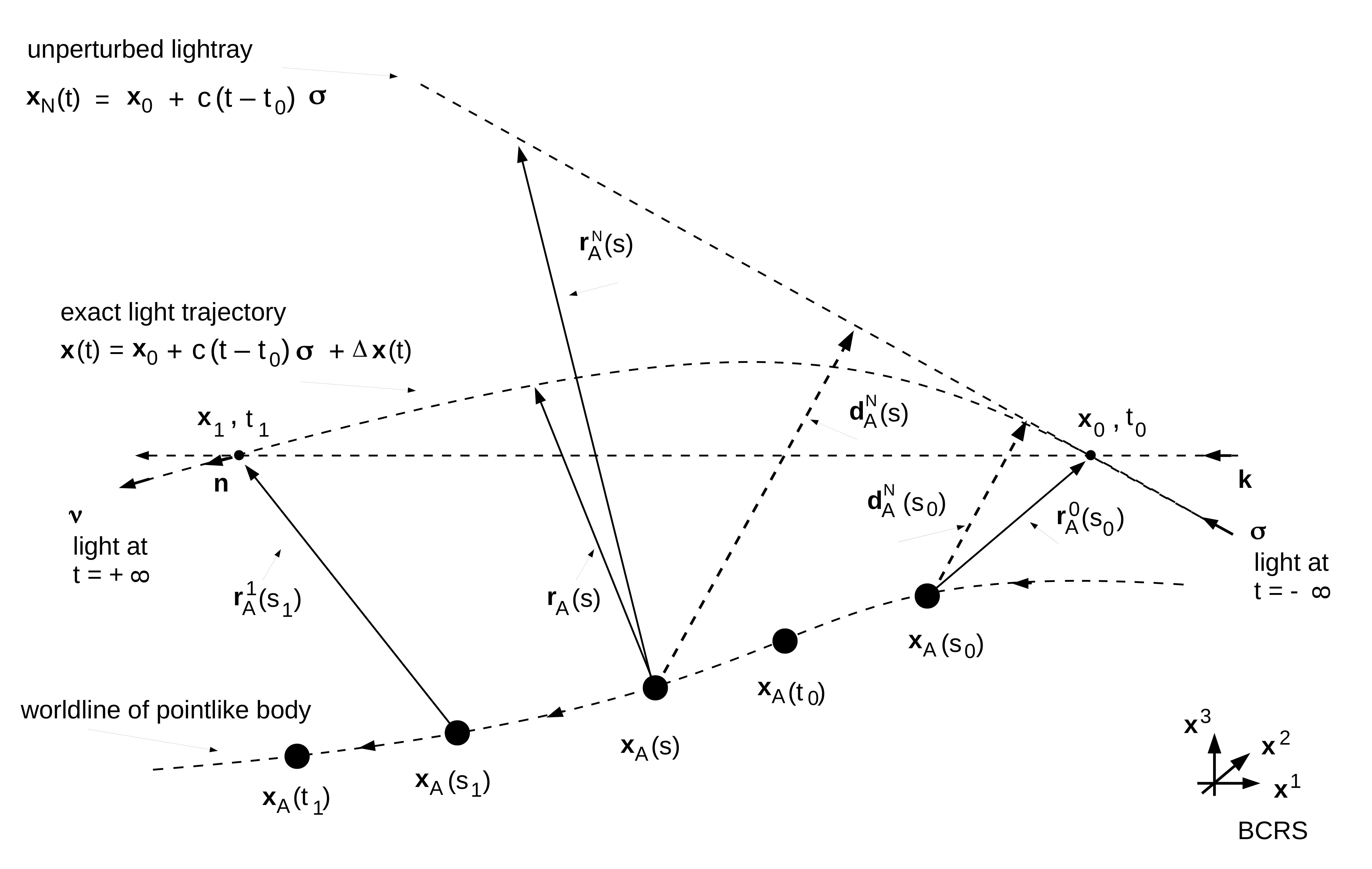 Figure 1
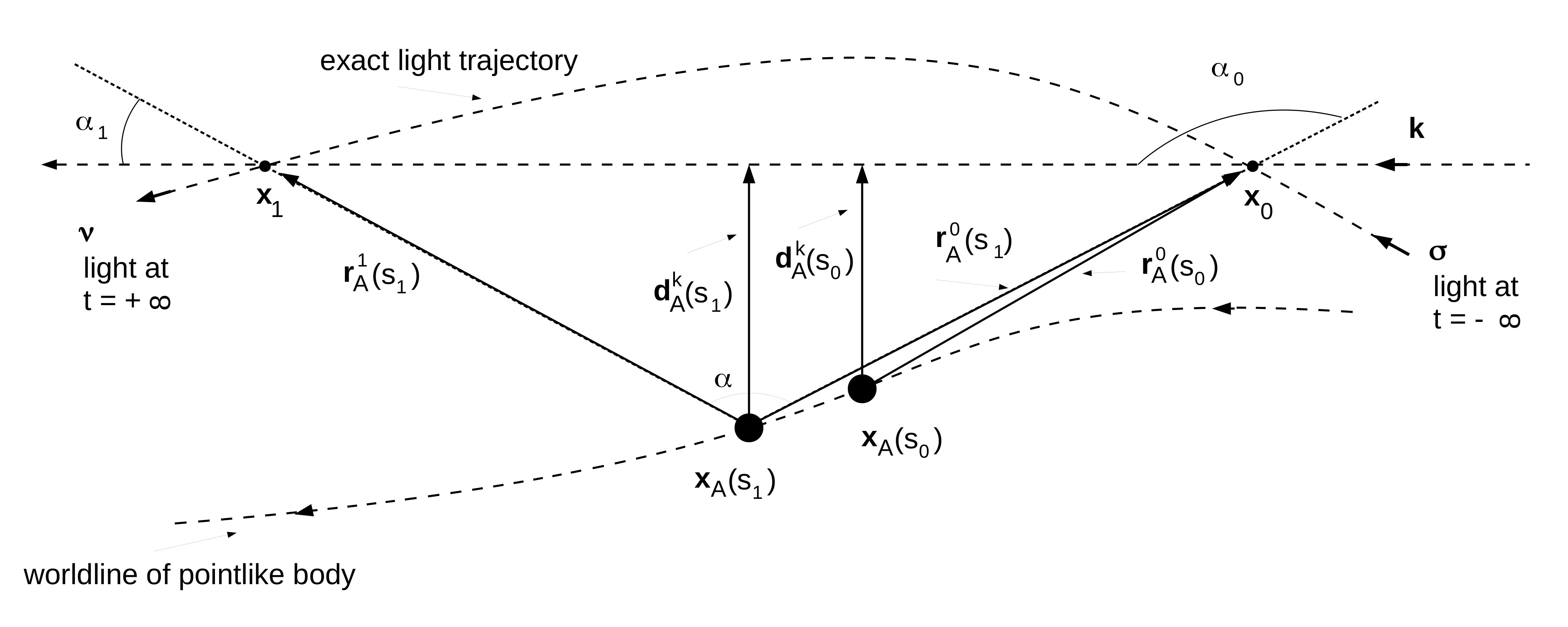 Figure 2
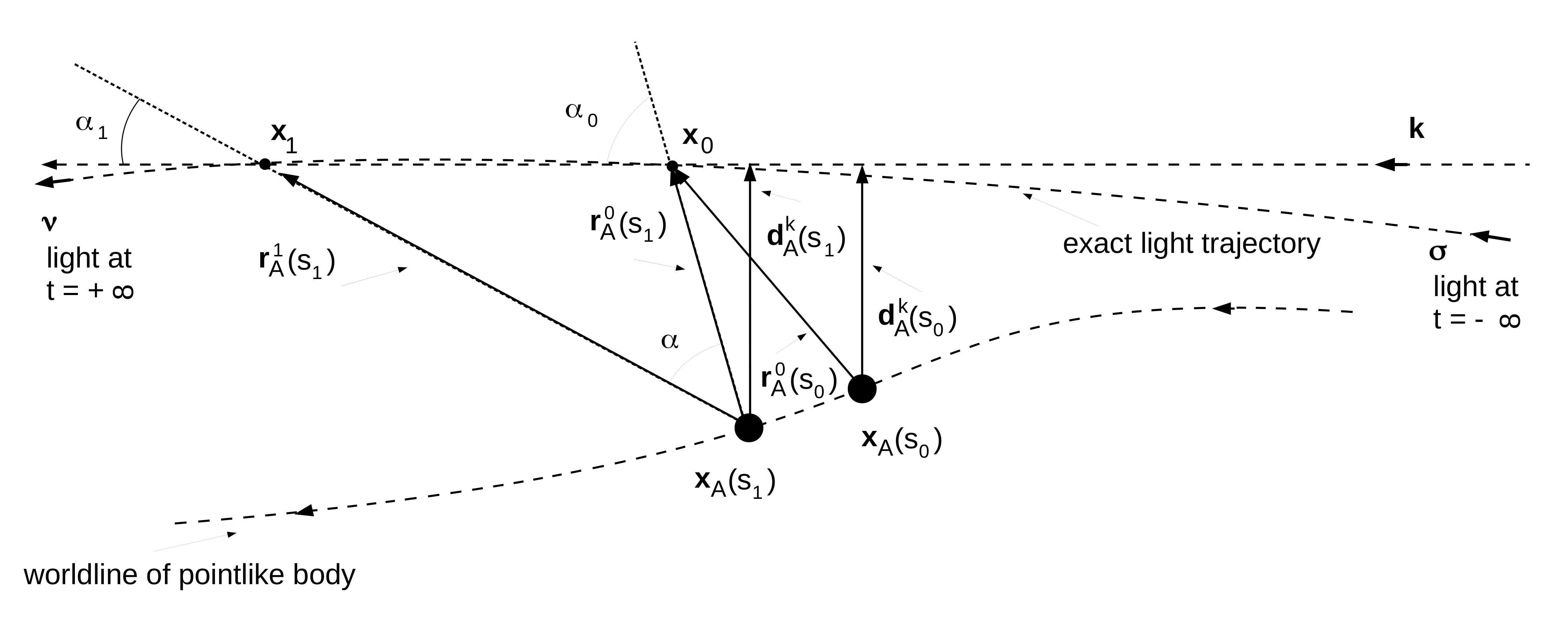 Figure 3
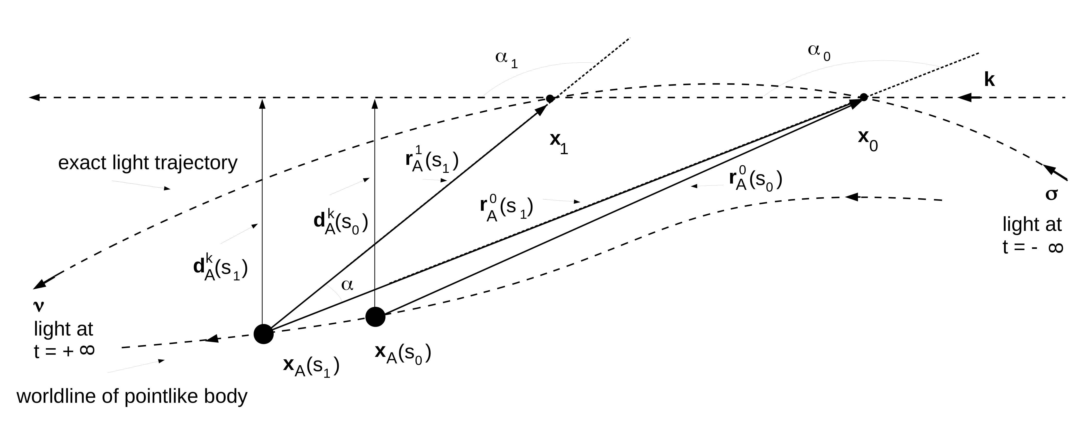 Figure 4
| Object | |||||
|---|---|---|---|---|---|
| Sun | |||||
| Mercury | |||||
| Venus | |||||
| Earth | |||||
| Mars | |||||
| Jupiter | |||||
| Saturn | |||||
| Uranus | |||||
| Neptune |
| Sun at | |||||||||
|---|---|---|---|---|---|---|---|---|---|
| Mercury | |||||||||
| Venus | |||||||||
| Earth | |||||||||
| Mars | |||||||||
| Jupiter | |||||||||
| Saturn | |||||||||
| Uranus | |||||||||
| Neptune |
| Sun at | ||||||||||
|---|---|---|---|---|---|---|---|---|---|---|
| Mercury | ||||||||||
| Venus | ||||||||||
| Earth | ||||||||||
| Mars | ||||||||||
| Jupiter | ||||||||||
| Saturn | ||||||||||
| Uranus | ||||||||||
| Neptune |
Peer Reviews
No public reviews on file for this paper yet. If you reviewed it on a platform where reviews are public (OpenReview, ICLR, NeurIPS, ICML), you can paste yours below so the community can read it here.
Videos
No videos yet. Explain this paper in a talk, walkthrough, or lecture? Add one.
Light propagation in 2PN approximation in the field of one moving monopole II. Boundary value problem
Sven Zschocke
Institute of Planetary Geodesy - Lohrmann Observatory, Dresden Technical University, Helmholtzstrasse 10, D-01069 Dresden, Germany
Abstract
In this investigation the boundary value problem of light propagation in the gravitational field of one arbitrarily moving body with monopole structure is considered in the second post-Newtonian approximation. The solution of the boundary value problem comprises a set of altogether three transformations: \mbox{\boldmathk}\rightarrow\mbox{\boldmath\sigma}, \mbox{\boldmath\sigma}\rightarrow\mbox{\boldmathn}, and \mbox{\boldmathk}\rightarrow\mbox{\boldmathn}. Analytical solutions of these transformations are given and the upper limit of each individual term is determined. Based on these results, simplified transformations are obtained by keeping only those terms relevant for the given goal accuracy of nano-arcsecond in light deflection. Like in case of light propagation in the gravitational field of one body at rest, there are so-called enhanced terms which are of second post-Newtonian order but contain one and the same typical large numerical factor. Finally, the impact of enhanced terms beyond 2PN approximation is considered. It is found that enhanced 3PN terms are relevant for astrometry on the level of nano-arcsecond in light deflection, while enhanced 4PN terms are negligible, except for grazing rays at the Sun.
pacs:
95.10.Jk, 95.10.Ce, 95.30.Sf, 04.25.Nx, 04.80.Cc
1 Introduction
1.1 The new era of space-based astrometry
While advancement in astrometry has always been benefited from ground-based telescope improvements, the new era of space-based astrometry missions has initiated unprecedented accuracies in positional measurements of celestial objects, like Solar System objects, stars, galaxies, and quasars [1, 2, 3]. Most notably, the astrometry missions Hipparcos and Gaia of the European Space Agency (ESA) have opened this new age in astronomy. These missions have (i) adapted from wide-field astrometry realized by optical instruments which are designed to measure large angles on the sky simultaneously, (ii) utilized the most modern technologies in the optical design of scanning satellite, (iii) taken advantage of appreciable developments in theoretical astrometry and applied gravitational physics.
Approved by ESA in 1980 and launched on 8 August 1989, Hipparcos was the first ever astrometric satellite to precisely measure the positions and proper motions of stars in the vicinity of the Sun. The completion of the Hipparcos mission has led to the creation of three highly accurate catalogues of stellar positions, namely the star catalogues Hipparcos and Tycho in 1997 [4, 5] and Tycho-2 in 2000 [6]. In particular, the Hipparcos final catalogue [4] provides astrometric positions and stellar motions up to milli-arcsecond () in angular accuracies for about thousand stars. The catalogues Tycho [5] and Tycho-2 [6] contain positions of about and stars, respectively, with an accuracy of up to in angular resolution which still represents an unprecedented accuracy at that time, also in view of such huge number of individual stars. These catalogues set the precedent on stellar positions and are continuously used in space science research and for spacecraft navigation.
Gaia is the second space-based mission ever and will provide fundamental data for many fields of astronomy. The Gaia mission was approved in 2000 by ESA as cornerstone mission and is aiming at precisions up to a few micro-arcseconds () in determining positions and proper motions of stellar objects [7], which is about times more accurately than the predecessor Hipparcos. Launched on 19 December 2013, the Gaia’s main goal is to create an extraordinarily precise three-dimensional map of more than million stars of our galaxy, in order to determine the structure and dynamics of the Milky way. The observational data of Gaia comprise not only astrometry but also spectro-photometry. For the brightest subset of targets, spectra will be acquired to obtain radial velocities of stellar objects by means of the Doppler effect which is essential for the understanding of the kinematics of our Galaxy [8].
The highly precise measurements of the astrometry mission Gaia are of fundamental importance to all the other fields of astronomy, specifically they will have a tremendous impact on stellar astrophysics and galaxy evolution, solar-system and extra-solar planet science, extra-galactic astrophysics, and fundamental physics like dark matter and dark energy physics, highly-precise determination of natural constants, testing equivalence principle, determination of Nordtvedt parameter, possible temporal variation of the gravitational constant, and last but not least testing alternative theories of gravity. Another aspect of highly-precise astrometric data concerns the essential fact that not only more accurate but also qualitatively new tests of general relativity become possible [9, 10, 11, 12].
Preliminary results of the Gaia mission have been published in September 2016 by Gaia Data Release 1 (Gaia DR1), providing astrometric data which are more precise than those in any of the former star catalogues [8, 13, 14]. The five-parameter astrometric solution (positions, proper motions, parallaxes) for about million stars in common between the Tycho-2 Catalogue and Gaia is contained in Gaia DR1.
The results of Gaia Data Release 2 (Gaia DR2) were published very recently in April 2018 by a series of articles. There are specific articles and processing papers which concern special scientific issues and which give technical details on the processing and calibration of the raw data. A comprehensive overview of Gaia DR2 is expounded in [15], while the full content of Gaia DR2 is available through the Gaia archive [16]. In particular, Gaia DR2 provides precise positions, proper motions, and parallaxes for more than million stars. Furthermore, the Gaia DR2 contains positions for more than thousand quasars which allow for the definition of a new celestial reference frame fully based on optical observations of extra-galactic sources (Gaia-CRF2) [17]. Based on these results the third realization of the International Celestial Reference Frame (ICRF-3) has recently been adopted by the XXXth General Assembly of the International Astronomical Union (IAU) in 2018 [18], which is based on the accurate measurement of over extragalactic radio sources. The ICRF-3 replaces ICRF-2 which was adopted at the XXVIIth General Assembly of IAU in 2009. These reference frames are of utmost importance for many branches is astronomy, like stellar catalogues, space navigations, or determination of the rotational motion of the Earth.
Of specific importance for our investigations here is the impressive advancement in astrometric accuracy of positional measurements arrived within the Gaia DR2. For parallaxes, uncertainties are typically around as for sources brighter than , around as for sources with a magnitude about , and around as for sources with about [15, 19]. These results represent a giant advancement in astrometric science and comprise the fact that todays astrometry has reached the micro-arcsecond level of accuracy in astrometric measurements.
Another astrometric space mission aiming at the micro-arcsecond level of accuracy is JASMINE, an approved long-term project developed by the National Astronomical Observatory of Japan, and which consists of altogether three astrometry satellites, called Nano-JASMINE, Small-JASMINE, and (Medium-Sized) JASMINE [20], where the two last satellites shall observe in the infrared. The Nano-JASMINE (nominal mission: years) is a mission in the optical based on CCD (charge-coupled device) and the technical demonstrator of the entire JASMINE project, which represents the first space astrometry satellite mission in Japan and the third space-based astrometry mission ever following the ESA missions Hipparcos and Gaia. Meanwhile, the technical equipment of the satellite has fully been completed and the launch of Nano-JASMINE is expected within the very few next months. The launch of Small-JASMINE is expected around 2024, while there is no concrete plan for the launch of (Medium-Sized) JASMINE. Within the series of altogether three JASMINE missions, the target accuracy in the positional measurements of stellar objects will be increasing step-by-step, ranging from by the Nano-JASMINE mission up to 10\,\hbox{\rm\muas} within the (Medium-Sized) JASMINE mission.
1.2 Future astrometry on the sub-micro-arcsecond level
It is quite obvious that a long term goal of astrometric science is to arrive at the sub-micro-arcsecond (sub-) or even the nano-arcsecond (nas) level of accuracy. The scientific objectives for such ultra-highly precise astrometry are overwhelming and it is almost impossible to enumerate all advances in science which astrometry on such scales would initiate. For instance, astrometry on sub- scale would make it possible to survey hundreds of thousands of stars up to a distance of about for detecting earth-like planets, would allow for much more stringent tests of General Relativity through light bending, would enable the measurement of the energy density of stochastic gravitational wave background, allows for precise mapping of dark matter from the areas beyond the Milky Way, enables direct distance measurement of various stellar standard candles up to the closest galaxy clusters, would allow for further tests of alternative theories of gravity with much better precision than in the weak-gravitational-field regime [21, 22, 23, 24, 25]. Especially, the proposed mission Theia [26] is primarily designed to study the local dark matter properties, the detection of Earth-like exoplanets in our nearest star systems and the physics of highly compact objects like white dwarfs, neutron stars, black holes. For a more comprehensive list of astronomical and astrophysical problems which can be solved by sub- astrometry we refer to the article [27].
Furthermore, as soon as the third (Gaia DR3) and final Gaia Data Release (Gaia Final DR), expected in the fall of 2020 and around the end of 2022, respectively, are achieved and analyzed, new questions will emerge, which will require new space-based astrometry missions, either in the form of a Gaia-like observer or in the form of satellites aiming at the sub- or even the nas level of accuracy. In fact, the impressive progress, made during the realization of the both ESA astrometry missions Hipparcos and Gaia, has already encouraged the astrometric science community to further proceed in such directions in foreseeable future. Among several astrometry missions suggested to ESA we mention the recent medium-sized (M-5) mission proposals Gaia-NIR [28], Theia [26], and NEAT [29, 30, 31], which in this order are aiming at the , sub-, and even the level of precision.
The envisaged advancement from as-astrometry to sub-as-astrometry implies many subtle effects and new kind of challenges in technology and science such as: (a) determination of Solar System ephemerides precisely enough for sub-as-astrometry, (b) modeling the influence of interstellar medium on light propagation, (c) synchronization of atomic clocks between observer and ground stations on the sub-nano-second scale, (d) tracking the spacecraft’s worldline and velocity with sufficient accuracy for being able to account for aberrational effects, (e) development of new CCD-based technologies in the optical or infrared to achieve astrometric data on the sub-as-level, etc. Each of these and many other challenges have to be clarified before sub-as-astrometry becomes feasible. But it is clear that astrometric information is mainly carried by light signals of the celestial light sources, hence astrometric measurements are intrinsically related to the problem about how to trace a light ray detected by the observer back to the celestial light source. Therefore, the fundamental assignment in astrometry remains the precise description of the trajectory of the light signal as function of coordinate time. The foreseen progress in the accuracy of observations and new observational techniques necessitates to account for several relativistic effects in the theory of light propagation. A detailed review about the recent progress in the theory of light propagation has been given in text books [10, 32] as well as in several articles [11, 33, 34, 35, 36, 37, 38, 39, 40]. So in what follows an introduction of the theory of light propagation is just given to the extent that it proves necessary for our investigations.
1.3 The exact field equations of gravity
According to the theory of general relativity [41, 42] the space-time is not considered as rigidly given once and for all, but a differentiable manifold and subject to dynamical laws. Therefore, the determination of the (inner) geometry of space-time is the foundation for any measurement in relativistic astrometry. The (inner) geometry of the four-dimensional manifold is fully determined by the metric tensor whose components are identified with tensorial gravitational potentials generalizing the scalar gravitational potential of Newtonian theory of gravity. In compliance with Einstein’s field equations [41, 42], the metric tensor is related to the stress-energy tensor of matter via a set of coupled non-linear partial differential equations given by [10, 41, 42, 43, 44, 45] (e.g. Sec. 17.1 in [43])
[TABLE]
where is the Ricci tensor (cf. Eq. (8.47) in [43]), is the Ricci scalar, and
[TABLE]
are the Christoffel symbols which are functions of the metric tensor.
The field equations of gravity (1) are valid in any coordinate system. The final ambition in theoretical astrometry remains of course the determination of observables (scalars), which are, by definition, gauge-independent (coordinate-independent) quantities [46]. There are three possibilities to get such observables [47]:
performing the calculations solely in terms of coordinate-independent quantities. 2. 2.
using any coordinate system in the calculations. 3. 3.
adopting one coordinate system and determine observables in the final step.
The IAU has adopted the third way by recommending the use of harmonic coordinates in celestial mechanics and in the astrometric science [48]. These harmonic coordinates considerably simplify the calculations in celestial mechanics and in the theory of light propagation. They are denoted by x^{\mu}=\left(ct,\mbox{\boldmathx}\right), where is the coordinate time and \mbox{\boldmathx}=\left(x^{1},x^{2},x^{3}\right) is a triplet of spatial coordinates. The harmonic coordinates are curvilinear and they are defined by the harmonic gauge condition [10, 32, 43],
[TABLE]
where is the determinant of metric tensor. The condition (3) is called de Donder gauge in honor of its inventor [49], which was also found independently by Lanczos [50]; we note that (3) determines (a class of) concrete reference systems, hence it is not surprising that condition (3) is not covariant. The harmonic coordinates can be treated like Cartesian coordinates besides that they are curvilinear [10, 32, 51, 52, 53]; cf. text below Eq. (3.1.45) in [32] or the statement above Eq. (1.1) in [51], while more detailed explanations for this fact are provided in Sections 1.5. and 1.6 in [53].
In line with these statements, in practical calculations in celestial mechanics and astrometry it is very useful to express the exact field equations of gravity (1) in terms of harmonic coordinates. In this so-called Landau-Lifschitz formulation of the field equations [44], the contravariant components of the gothic metric density are decomposed as follows
[TABLE]
which is especially useful in case of an asymptotically flat space-time. Here, is the trace-reversed metric perturbation which describes the deviation of the gothic metric tensor density of curved space-time from the metric tensor of Minkowskian space-time.
The exact field equations (1) in terms of harmonic coordinates can be written as follows (cf. Eq. (36.37) in [43] or Eq. (5.2b) in [51]):
[TABLE]
where is the (flat) d’Alembert operator and
[TABLE]
where is the Landau-Lifschitz pseudotensor of gravitational field [44], which is symmetric in the indices and in explicit form given by Eq. (20.22) in [43] or by Eqs. (3.503) - (3.505) in [10]. We shall assume that the gravitational system is isolated, that means flatness of the metric at spatial infinity and the constraint of no-incoming gravitational radiation is imposed at past null infinity (cf. notation in Section 34 in [43] and Figure 34.2. in [43]). These so-called Fock-Sommerfeld boundary conditions, for instance given by Eqs. (4.64) and (4.65) in [10], have been adopted from classical electrodynamics [54, 55] and later formulated for the general theory of gravity [45]. By imposing the Fock-Sommerfeld boundary conditions, a formal solution of (5) is then provided by the implicit integro-differential equation,
[TABLE]
where
[TABLE]
is the retarded time, which is associated with the finite speed of gravitational action and not with the finite speed of light, as one may recognize from the fact that electromagnetic fields are not necessarily involved in the stress-energy tensor on the r.h.s. of (5) or (8). In order to deduce the formal solution (8) from the differential equation (5) the Cartesian-like harmonic coordinates \left(ct,\mbox{\boldmathx}\right) have been treated like Cartesian coordinates besides that they are curvilinear; cf. text below Eq. (36.38) in [43]. The approach about how to solve (8) iteratively is described in some detail in [10]; cf. Eqs. (3.530a) - (3.530d) in [10]. In the first iteration (first post-Minkowskian approximation) the integral runs only over the three-dimensional volume of the matter source, while from the second iteration on (second post-Minkowskian approximation and higher) the integral (8) gets also support from the metric perturbation, hence runs over the entire three-dimensional space.
Four comments are in order about the exact field equations of gravity.
First, the retarded time , which is hidden in the exact field equations of gravity (1), appears explicitly in the formal solution of the exact field equations (8), which states that a space-time point \left(u,\mbox{\boldmathx}^{\prime}\right) (e.g. located inside the matter distribution) is in causal contact with a space-time point \left(t,\mbox{\boldmathx}\right) (e.g. located outside the matter source).
Second, one may consider the propagation of electromagnetic action in a curved space-time with background metric . That means, the metric of the curved space-time is determined by some matter distribution , while the impact of the electromagnetic field on the metric of space-time is neglected. The electromagnetic fields are generated by some electromagnetic four-current j^{\mu}=\left(c\rho,\mbox{\boldmathj}\right) with and being charge-density and current-density, respectively. The covariant field equations of Maxwell’s electrodynamics in curved space-time read and (cf. Eqs. (22.17a) and (22.17b) in [43]), where is the field-tensor of electromagnetic field (cf. Eq. (22.19a) in [43]), the semicolon denotes covariant derivative, and A^{\mu}=\left(\varphi/c,\mbox{\boldmathA}\right) is the four-potential, where is the scalar potential and is the vector potential. The Characteristics (also called characteristical surface) of the covariant Maxwell equations are governed by the following non-linear partial differential equation (non-linear PDE) of first order [45, 56, 57, 58, 59],
[TABLE]
which is valid in the near-zone as well as in the far-zone of the four-current j^{\alpha}\left(t,\mbox{\boldmathx}\right) and is valid in any reference system. The Characteristics are three-dimensional curved sub-manifolds, , of the Riemannian space-time. In case of flat space-time, i.e. , the characteristical surface at the event is given by the Minkowskian light-cone,
[TABLE]
That means, an electromagnetic discontinuity (abrupt electromagnetic signal) generated at propagates in the flat space-time along the light-cone (11). The generalization of the light-cone (11) in flat space-time is the light-conoid in curved space-time as governed by Eq. (10), which for the curved space-time of the Solar system can only be solved approximately, for instance by iteration. The PDE of the Characteristics (10) can be derived by means of the following consideration. Let be a continuous (smoothly changing) electromagnetic four-potential generated by some current somewhere located in the Riemannian space-time with metric . Now suppose that the four-current changes rapidly and generates an abrupt Theta-like discontinuity (perturbation) in the electromagnetic field with amplitude , which propagates along some hypersurface . Then, the entire electromagnetic four-potential is given by the following expression: A^{\mu}\left(x^{0},\mbox{\boldmathx}\right)=a^{\mu}\left(x^{0},\mbox{\boldmathx}\right)+u^{\mu}\left(x^{0},\mbox{\boldmathx}\right)\,\Theta\left(\phi\left(x^{0},\mbox{\boldmathx}\right)\right) [58]. By inserting this ansatz into the covariant Maxwell equations one just obtains the equation (10) which governs the evolution of the hypersurface in the curved space-time on which any discontinuity of the electromagnetic field is located. Thus, the three-dimensional sub-manifolds of the Riemannian space-time can be identified with the front of electromagnetic action (e.g. abrupt discontinuity in the near-zone of the four-current or wave-front of an electromagnetic wave in the far-zone of the four-current) caused by some rapid change in the electromagnetic four-current.
Furthermore, one may introduce a trajectory, where is an affine curve-parameter, which is orthogonal on the surface [45, 57, 58, 59],
[TABLE]
that means is normal to the front of electromagnetic action; we will come back to that issue later, cf. text below Eqs. (66) - (68). Such trajectories are called Bicharacteristics. The Bicharacteristics can be identified with the light rays, which propagate with the finite speed of light. Therefore, also the Characteristics, that is the surface of electromagnetic action, propagates with the finite speed of light. The light-conoid in curved space-time is built by all Bicharacteristics emanating from some (arbitrary) event. As mentioned above, besides that is defined as the fundamental speed of light in vacuum in the flat Minkowski space, it is clear that the retardation, that means the natural constant in the denominator on the r.h.s. in Eq. (9), is caused by the finite speed of gravitational action and not due to the finite speed of light. Even in case the stress-energy tensor of matter would only consist of electromagnetic fields, [43], then, nevertheless, the retardation would also originate from the finite speed of gravitational fields (in this case with the well-known property that the Ricci scalar vanishes but of course not the Ricci tensor) which, in this specific case, would entirely be generated by these electrodynamical fields.
Third, let us now consider the non-linear PDE for the Characteristics of the exact field equations of gravity (1), which is given by [45, 57, 58, 59],
[TABLE]
which is valid in the near-zone as well as in the far-zone of the matter source T_{\alpha\beta}\left(t,\mbox{\boldmathx}\right) and is valid in any reference system. The derivation of the PDE (13) for the Characteristics is similar to the above considerations in case of the covariant Maxwell equations. Consider a continuous (smoothly changing) background metric which is generated by some matter . Then assume a rapid acceleration of the matter which results in an abrupt Theta-like discontinuity (perturbation) with metric . Hence, the entire metric is given by: g^{\alpha\beta}\left(x^{0},\mbox{\boldmathx}\right)=g^{\alpha\beta}_{0}\left(x^{0},\mbox{\boldmathx}\right)+h^{\alpha\beta}\left(x^{0},\mbox{\boldmathx}\right)\,\Theta\left(\omega\left(x^{0},\mbox{\boldmathx}\right)\right) [58]. Now, if one wants to investigate how the gravitational discontinuity (non-analytic gravitational signal) propagates in space and time, one has to insert this ansatz into the exact Einstein equations, which yields the PDE (13). Thus, the Characteristics can be identified with the front of gravitational action (e.g. abrupt discontinuity in the near-zone of matter source or wave-front of a gravitational wave in the far-zone of matter source) caused by the matter source. The front of gravitational action is a curved three-dimensional sub-manifold, , of the Riemannian space-time, that means a three-dimensional surface on which any discontinuities of the gravitational field must lie [45, 57, 58, 59]. In case of flat background metric, i.e. , the solution of the PDE (13) at the event is given by the null-cone,
[TABLE]
That means, a gravitational discontinuity (abrupt gravitational signal) generated at propagates in the flat space-time along the null-cone (14). The generalization of the null-cone (14) of gravitational action in flat background metric is the null-conoid in curved space-time as governed by (13), which for the curved space-time of the Solar system can only be solved approximately, for instance by iteration.
One may also introduce Bicharacteristics for the field equations of gravity, where is an affine curve-parameter, which are trajectories orthonormal on the hypersurface [45, 57, 58, 59],
[TABLE]
that means is normal to the front of gravitational action; we will come back to that issue later, cf. text below Eqs. (66) - (68). These Bicharacteristics can be considered as gravitational rays. Such an idealized picture is well justified for a gravitational wave when the wavelength is negligibly small in comparison with the spatial region of propagation of the wave. Such condition is satisfied in the far-zone of the Solar System, but not in the near-zone of the Solar System where the wavelength of gravitational radiation is larger than the boundary of the near-zone. That is why the Bicharacteristics in the near-zone should be considered as a mathematical concept of being normals onto the characteristic hypersurface , while in the far-zone the Bicharacteristics can physically be interpreted as gravitational rays. But what is important here is the fact that the speed of gravity equals the speed of light, because the equations (10) and (12) are identical with (13) and (15), respectively; cf. Section 7.2 in [10]. Therefore, as just mentioned above, the natural constant in the denominator on the r.h.s. in Eq. (9) is related to the finite speed of gravity which equals the finite speed of light. The null-conoid (at some arbitrary event), can also be defined as the set of all Bicharacteristics emanating from that (arbitrary) event in the curved space-time.
Fourth, as stated above, the equations for the Characteristics, Eq. (10) and Eq. (13), are fundamental consequences of the exact field equations of electrodynamics in curved space-time and the exact field equations of gravity, respectively. They state that there is no difference between the speed of light in curved space-time and the speed of gravitational action; cf. §53 in [45]. Nevertheless, the propagation of electromagnetic action and the propagation of gravitational action are two different physical processes, and besides that their velocities are numerically equal, it does not mean that they can not be distinguished from each other. For instance, if the directions of electromagnetic wave propagation and propagation of gravitational action are different from each other, then one may distinguish between the directions of both these velocities; cf. Section 7.2 in [10]. Furthermore, the important theoretical prediction of Einstein’s theory that both velocities are equal to each other, has recently been confirmed by the first detection of gravitational waves generated by the inspiral and merger of a binary neutron star and the determination of the location of the source by subsequent observations in the electromagnetic spectrum [60, 61]. This measurement has constrained the difference between the speed of gravity and the speed of light to be between and times the speed of light [62]. Needless to say that in this case both physical processes have clearly been separated, besides that the gravitational wave and the electromagnetic signal were parallel to each other.
A detailed description about how the finite speed of gravity in the near-zone of the Solar System could in principle be determined by means of Very Long Baseline Interferometry (VLBI) has been presented in [63]. The suggested approach is based on the increasing precision of VLBI facilities which allow to determine the impact of the orbital velocity \mbox{\boldmathv}_{A} of a massive Solar System body on the Shapiro time-delay, which states that the total time of the propagation of a light signal from the four-coordinate of a light source \left(ct_{0},\mbox{\boldmathx}_{0}\right) to the four-coordinate of an observer \left(ct_{1},\mbox{\boldmathx}_{1}\right) is given by (e.g. Eq. (43) in [37])
[TABLE]
where \left|\mbox{\boldmathx}_{1}-\mbox{\boldmathx}_{0}\right| is the Euclidean distance between source and observer and is the time-delay of the light signal caused by the gravitational field of the massive body in motion.
In the first post-Minkowskian (1PM) approximation, which is exact up to terms to order and exact to all orders in the speed of the body, the time-delay is given by Eq. (51) in [37], which, by neglecting all terms proportional to the acceleration of the body (series expansion (35) is also employed), reads:
[TABLE]
which is valid for light propagation in the field of one monopole in arbitrary motion, irrespective of the fact that acceleration terms of the body were neglected. The unit-vector points from the light source towards the position of the observer, and the three-vectors \mbox{\boldmathr}_{A}\left(s_{0}\right)=\mbox{\boldmathx}\left(t_{0}\right)-\mbox{\boldmathx}_{A}\left(s_{0}\right) and \mbox{\boldmathr}_{A}\left(s_{1}\right)=\mbox{\boldmathx}\left(t_{1}\right)-\mbox{\boldmathx}_{A}\left(s_{1}\right), where \mbox{\boldmathx}\left(t_{0}\right) and \mbox{\boldmathx}\left(t_{1}\right) are the spatial coordinates of the light signal at source and observer, respectively, while \mbox{\boldmathx}_{A}\left(s_{0}\right) and \mbox{\boldmathx}_{A}\left(s_{1}\right) are the spatial position of the body at the retarded time and , as defined in the below standing equations (45) and (47). Let us notice here that (17) also agrees with Eqs. (146) - (148) in [34].
In the 1.5 post-Newtonian (1.5PN) approximation, which is exact up to terms to order that means only exact to the first order in the speed of the body, the time-delay is given by Eq. (7) in [64] and reads:
[TABLE]
which is valid for light propagation in the field of one monopole in uniform motion, that means all acceleration terms of the body are zero. The three-vectors \mbox{\boldmathr}_{A}\left(t_{0}\right)=\mbox{\boldmathx}\left(t_{0}\right)-\mbox{\boldmathx}_{A}\left(t_{0}\right) and \mbox{\boldmathr}_{A}\left(t_{1}\right)=\mbox{\boldmathx}\left(t_{1}\right)-\mbox{\boldmathx}_{A}\left(t_{1}\right), where \mbox{\boldmathx}_{A}\left(t_{0}\right) and \mbox{\boldmathx}_{A}\left(t_{1}\right) are the spatial positions of the body at time of emission and time of reception of the light signal. Furthermore, in Eq. (18) the three-vector \displaystyle\mbox{\boldmathK}=\mbox{\boldmathk}-\mbox{\boldmathk}\times\left(\frac{\mbox{\boldmathv}_{A}}{c}\times\mbox{\boldmathk}\right). Let us notice here that Eqs. (137) - (139) in [34] are valid for light propagation in the field of one arbitrarily moving body in slow motion, which in case of uniform motion coincide with (18), as one may show by series expansion.
For grazing light rays or radio waves at massive bodies of the Solar System, the velocity dependent terms in (17) or (18) contribute of the order of a few picoseconds in time-delay; cf. Table II in [34] for grazing rays at Sun or giant planets. At this order of precision it becomes possible to measure such velocity-dependent terms in time-delay (17) or (18) by means of the most modern VLBI techniques. In fact, such a concrete experiment by VLBI facilities has been suggested in [63], and has finally been performed in 2002 with remarkable effort and precision [66]. In particular, in [66] the Shapiro time delay of a radio wave, emitted by the quasar and passing near Jupiter, has been determined with extremely high precision, in order to determine the finite speed of the gravity fields of that moving body. This experiment has, at the very first time, succeeded in determining the impact of the orbital velocity effects to order of Jupiter on the Shapiro time-delay. Subsequently, these results have initiated a controversial debate in the literature about the correct interpretation of this experiment [9, 64, 65, 67, 68, 69, 70, 71, 72, 73, 74, 75, 76, 77, 78, 79]; further comments about the Kopeikin-Formalont experiment can be found in [10, 80, 81, 82, 83]. While there is no doubt at all in the literature about the correctness of the expressions (17) and (18), a central topic of this conversion was about the correct physical meaning of the natural constant in the velocity-dependent terms in (17) and (18).
That remarkable debate had arisen just because of the above discussed fundamental prediction of general relativity that the speed of gravity and the speed of light are numerically equal. That is why it becomes a highly sophisticated assignment of a task to disentangle these both velocities in concrete astrometrical measurements. In [37] it was shown that the retarded instant of time and in (17) are caused by the retarded time of the Liénard-Wiechert potential of the metric tensor (Eq. (10) in [37]), hence they are caused by the finite speed of gravity so that the natural constant is related to the finite speed of gravity. And due to the fact that (18) can be deduced from (17) by series expansion and by assuming a uniform motion of the body, one might be inclined to assume that the natural constant in (18) is related to the finite speed of gravity. On the other side, in [64] it was shown that the natural constant in (18) is caused by the finite speed of light and is not related to the finite speed of gravity. So it might be that a unique interpretation of the experiment is impossible as long as one is restricted to terms of the first order in . But it should be noticed that the controversy was not about the correctness of the theory of general relativity, but mainly about the question of whether the velocity-dependent term in the Shapiro time-delay is related to the finite speed of gravity (retardation of gravitational action) or to the finite speed of light (aberration of light).
In this context it should also be noticed that there is agreement among the participants of this controversy with respect to the following minimal set of issues:
- (a)
the retarded time in (9) is caused by the finite speed of gravity. 2. (b)
the finite speed of gravity has surely an impact on the Shapiro time-delay. 3. (c)
the impact of orbital velocity of Jupiter on time-delay has been detected in [66].
While in principle the experiment suggested in [63] is capable to measure the speed of gravity, there is no general consensus about the correct interpretation of the results of the concrete experiment in [66], as it was also formulated in [81]. It seems that the fact that the retarded time in (9) as well as the retarded time and in the below standing equations (45) and (47) are due to the finite speed of gravity might not necessarily be convincing for a unique and correct interpretation of these astrometrical VLBI measurements [64]. Moreover, in [64] it was argued that acceleration terms or terms of the order give the first level at which retardation effects due to the motion of the massive bodies occur. However, in order to determine the next higher order terms, that means terms proportional to the acceleration of the body or terms of the order in the Shapiro time-delay, one needs to improve the precision in time measurements by VLBI experiments by a factor of about , which requires an ultra-high precision in the time-resolution of VLBI measurements of about , which is far out of reach of present-day VLBI facilities. Furthermore, the theoretical interpretation of the experiment might also depend on the generalized theoretical models beyond general relativity which allow to distinguish between the speed of light and speed of gravity [71]. Even the semantics in use could have an impact on the correct interpretation of these VLBI results [80]. Here, also in view of the exceptional number of articles in the literature related to this subject, a detailed and correct interpretation of this famous experiment would be far beyond the intention of our investigation. For the moment being, it seems sensible to keep in mind the problem and to realize that further careful investigations and higher precisions in VLBI measurements are necessary in order to clarify such involved difficulties regarding the distinction between the speed of electromagnetic fields and the speed of gravitational action in the near-zone of the Solar System.
Finally, having said all that we emphasize again that the retarded instant of time (9) originates from the finite speed of gravity which equals the speed of light, a fact that is in meanwhile sufficient for our considerations here; cf. also the comments in the text below Eqs. (31) and (34) as well as in the text below Eqs. (45) and (47).
1.4 The exact geodesic equation for light propagation
Throughout the investigation the propagation of a light signal in vacuum is considered. The most simplest light tracking model presupposes a four-dimensional flat space-time with Minkowskian metric which implicitly involves Cartesian coordinates, where the light ray propagates along a straight line. Then, a light signal emitted at some spatial point \mbox{\boldmathx}_{0} at time propagates along it’s initial direction , so that the light trajectory in the global system reads as follows,
[TABLE]
where suffix labels Newtonian approximation. Such a simple light propagation model is not sufficient for todays precision of astrometric measurements which, as stated above, implicates a corresponding advancement in the theory of light propagation. Especially, relativistic astrometry has necessarily to account for the fact that the space-time is not flat but a four-dimensional curved manifold. Because the space-time is curved, a light signal propagates along a geodesic which is the generalization of the concept of a straight line because a geodesic is a curve that parallel-transports its own tangent vector. Consequently, a fundamental assignment in relativistic astrometry concerns the precise modeling of the time track of a light signal through the curved space-time of Solar System, that is to say the determination the trajectory of the light signal, \mbox{\boldmathx}\left(t\right), in some reference system which covers the entire curved space-time (at least those part of the entire space-time which contains the light source and the observer) and, therefore, is called global coordinate system.
The trajectory of a light signal propagating in curved space-time is determined by the geodesic equation and isotropic condition, which in terms of coordinate time read as follows [10, 32, 43] (e.g. Eqs. (3.220) - (3.224) in [10]):
[TABLE]
where a dot denotes total derivative with respect to coordinate time, hence are the three-components of the coordinate velocity of the photon. The null condition (21) and geodesic equation (20) have equivalent physical content because (21) is a first integral of (20). As mentioned above, the natural constant explicitly seen in both these equations (20) and (21) means actually the speed of light, while the natural constant contained in the Christoffel symbols and metric tensor is related to the finite speed of gravity as stated already in the text below Eqs. (8) and (9). Furthermore, it should be mentioned that the coordinate velocity of a light signal in the global system of curved space-time differs from the speed of light in flat space-time \left|\dot{\mbox{\boldmathx}}\right|\neq c\,; only in the local system of a free-falling observer both are equal.
1.4.1 The initial value problem
The light signal is assumed to be emitted at the four-position of the light source, \left(t_{0},\mbox{\boldmathx}_{0}\right), as given in some global coordinate system \left(t,\mbox{\boldmathx}\right). Then, a unique solution of the partial differential equation (20) is well-defined by the so-called initial-value problem (Cauchy problem), where the spatial position of the light source, \mbox{\boldmathx}_{0}, and the initial unit direction of the light ray, \mbox{\boldmath\mu}=\dot{\mbox{\boldmathx}}\left(t_{0}\right)/\left|\dot{\mbox{\boldmathx}}\left(t_{0}\right)\right|, are given. Usually, the initial value problem is often replaced by the so-called initial-boundary conditions [10, 32, 35, 36, 38, 33, 34]:
[TABLE]
with being the unit-direction (\mbox{\boldmath\sigma}\cdot\mbox{\boldmath\sigma}=1) of the light ray at past null infinity (cf. notation in Section 34 in [43] and Figure 34.2. in [43]). The advantage for using initial-boundary conditions (22) rather than initial-value conditions when integrating the geodesic equation (20) is solely based on the integration constant which becomes simpler at past null infinity. One may easily find a unique relation between the tangent vectors and (e.g. Section 3.2.3 in [32]), so one verifies that there is a unique one-to-one correspondence between the initial-boundary problem (22) and the initial-value problem; more precisely, these statements are valid in case of a weak gravitational field and ordinary topology of space-time. According to (22), the solution for the light trajectory is a function of these initial-boundary conditions: \mbox{\boldmathx}\left(t\right)=\mbox{\boldmathx}\left(t,\mbox{\boldmathx}_{0},\mbox{\boldmath\sigma}\right).
1.4.2 The boundary value problem
A unique solution of geodesic equation (20) can also be defined by the so-called boundary-value problem rather than the initial-boundary problem (22). In the boundary-value problem a light signal is supposed to be emitted at some initial space-time point \left(t_{0},\mbox{\boldmathx}_{0}\right) (source) which is received at another space-time point \left(t_{1},\mbox{\boldmathx}_{1}\right) (observer) [10, 11, 12, 32, 35, 39]:
[TABLE]
Accordingly, the solution of the light trajectory will be a function of these boundary conditions: \mbox{\boldmathx}\left(t\right)=\mbox{\boldmathx}\left(t,\mbox{\boldmathx}_{0},\mbox{\boldmathx}_{1}\right).
Because in reality any light source is located at some finite distance, the solution of the boundary-value problem is of decisive importance in practical astrometry [10, 32, 35]. Accordingly, the primary aim of our investigation is to determine the solution of the boundary-value problem (23) when the solution of the initial-boundary problem (22) is given.
1.5 The geodesic equation for light propagation in 2PN approximation
The metric enters the geodesic equation (20) in virtue of the Christoffel symbols (2). It is, however, impossible to determine the Solar System metric without taking recourse to an approximation scheme. Such an approximative approach is possible, because in the Solar System the gravitational fields are weak, (Schwarzschild radius with and being mass and equatorial radius of body ) and the motions of matter are slow as compared with the speed of light (we have in mind that is just the orbital velocity of the body, but in general could also be rotational motion of extended bodies, convection currents inside the massive bodies, oscillations of the bodies, etc.). Accordingly, a series expansion in inverse powers of the natural constant is meaningful,
[TABLE]
where are tiny perturbations of the flat Minkowskian metric, that is for any . Here, in line of the comments made above regarding the physical meaning of the natural constant , we just notice that the post-Newtonian expansion of the metric tensor (24) is of course an expansion with respect to the inverse power of the speed of gravity.
The series expansion (24) includes all terms up to the fifth order and is called post-post-Newtonian (2PN) approximation of the metric tensor. The validity of the post-Newtonian expansion (24) is restricted to the near-zone region of the Solar System where the retardations are small by definition [10, 43, 52, 53, 84]; see also the Fig. 7.7 in [10] or Fig. 36.3 in [43]. The near-zone of a gravitating system is defined as spatial region with the boundary \left|\mbox{\boldmathx}\right|\ll\lambda_{\rm gr}\,, where is a characteristic wavelength of gravitational waves emitted by the system and the origin of spatial axes is assumed to be located at the center-of-mass of the gravitational system or somewhere nearby. For the Solar System one obtains about which is the lowest wavelength of gravitational radiation emitted by Jupiter during its revolution around the barycenter of the Solar System [10, 34, 43]. A more accurate statement is achieved by the fact that the term near-zone is intrinsically connected with orbital accelerations of the massive bodies which constitute gravitational system. In mathematical terms it requires
[TABLE]
for each massive body ; here is the orbital velocity and r_{A}\left(t\right)=\left|\mbox{\boldmathx}-\mbox{\boldmathx}_{A}\left(t\right)\right| is the spatial distance of some field point from the massive body located at \mbox{\boldmathx}_{A}\left(t\right). The condition (25) has already been stated by by Eq. (B7) in [85] or Eq. (97) in [86] and follows from , where the metric coefficients for a system of moving monopoles are given by Eqs. (24) - (27) in [86] 111Let us recall that the harmonic gauge condition (3) still inherits a residual gauge freedom, so the harmonic coordinates actually refer to a class of reference systems. A unique choice of harmonic coordinates is provided by the Barycentric Celestial Reference System (BCRS) [48], which defines the origin of spatial coordinates at the barycenter of the Solar System, a stipulation which removes the residual gauge freedom. The metric coefficients for a system of moving monopoles, which have been presented by Eqs. (24) - (27) in [86], are given in the BCRS, so they do not contain any gauge terms.. Using the numerical values of the most massive Solar System bodies as given in Table 1 we find the spatial radius of the near-zone to be about
[TABLE]
The results and considerations of our investigation are valid within this spatial region, which corresponds to about light-days.
By inserting the post-Newtonian expansion of the metric tensor (24) into the geodesic equation (20) via the Christoffel symbols (2) one obtains the geodesic equation in the so-called post-post-Newtonian (2PN) approximation, which is given, for instance, in [86, 85, 87]. The formal solution of the geodesic equation in 2PN approximation reads 222The notation in Eq. (27) has been adjusted to the standard notation commonly used in the literature [32, 33, 34, 85, 86]. A reconcilable notation for the series expansions (24) and (27) can be achieved by noticing that \Delta\mbox{\boldmathx}^{\left(2\right)}\equiv\Delta\mbox{\boldmathx}^{1{\rm PN}} and \Delta\mbox{\boldmathx}^{\left(3\right)}\equiv\Delta\mbox{\boldmathx}^{1.5{\rm PN}} and \Delta\mbox{\boldmathx}^{\left(4\right)}\equiv\Delta\mbox{\boldmathx}^{2{\rm PN}}.,
[TABLE]
The first two terms on the r.h.s. in (27) represent the unperturbed light ray (19), while the subsequent terms represent corrections to the unperturbed light ray. The physical meaning of the natural constant in the unperturbed light ray, \mbox{\boldmathx}_{0}+c\left(t-t_{0}\right)\mbox{\boldmath\sigma}, is of course the speed of light in flat Minkowskian space-time; cf. comment below Eqs. (20) - (21) regarding the geodesic equation and isotropic condition for light rays. It should be noticed that the post-Newtonian correction terms \Delta\mbox{\boldmathx}^{n{\rm PN}}\left(t\right) originate from the post-Newtonian expansion of the metric tensor (24), which is an expansion in inverses powers of , meaning the speed of gravity. However, in order to compute these correction terms \Delta\mbox{\boldmathx}^{n{\rm PN}}\left(t\right), the integration of geodesic equation proceeded along the unperturbed light ray [85, 86], where the meaning of is the speed of light. Therefore, the correction terms \Delta\mbox{\boldmathx}^{n{\rm PN}}\left(t\right) in (27) contain the natural constant in two different meanings, namely the speed of light and the speed of gravity. One might believe that this kind of entanglement makes it impossible to separate the impact of the finite speed of gravity and the finite speed of light in these correction terms. This is, however, not true. The terms related to the characteristics of the gravity field and the terms related to the light characteristics can clearly be separated in the solution of the light-ray trajectory (27); cf. comments below Eqs. (66) - (68).
For an overview of the state-of-the-art in the theory of light propagation we refer to the text books [10, 32] and the articles [11, 33, 34, 35, 36, 37, 38, 39, 40]. According to these references, an impressive progress in the determination of the correction terms \Delta\mbox{\boldmathx}^{1{\rm PN}}\left(t\right) and \Delta\mbox{\boldmathx}^{1.5{\rm PN}}\left(t\right) has been made during recent decades.
On the other side, the knowledge of the correction terms \Delta\mbox{\boldmathx}^{2{\rm PN}}\left(t\right) is pretty much limited thus far. In fact, the problem of light propagation in 2PN approximation, that means the determination of the light trajectory (27) as function of coordinate time, has only been considered for the following rather restricted situations 333Let us notice here that the light deflection in 2PN approximation in the field of one monopole at rest has been determined a long time ago [88, 89, 90, 91, 92, 93, 94]. But a unique interpretation of astrometric observations requires the knowledge of the propagation of the light signal, i.e. the determination of the light trajectory as function of coordinate time (27). We also notice the investigation in [95] where the problem of time delay in the field of one monopole in uniform motion has been considered, but this investigation was not aiming at astrometric measurements in the Solar System.:
2PN light trajectory in the field of one monopole at rest [32, 96] 444The results of [32, 96] were later confirmed in several related investigations [97, 98, 99, 100, 101, 102, 103, 104, 105, 106]., 2.
2PN light trajectory in the field of two point-like bodies in slow motion [87],
where [87] was not intended for light propagation in the Solar System.
It is, however, clear that for astrometry on the micro-arcsecond and sub-micro-arcsecond level it is indispensable to determine the light trajectory in the second post-Newtonian approximation for more realistic gravitational systems, especially where the motion of the bodies is taken into account [25, 97, 98, 99, 107, 108, 109, 110, 111]. Already for micro-arcsecond astrometry it is necessary to account for the motion of the Solar System bodies, where it is sufficient to determine the light trajectory in the field of one monopole at rest, \mbox{\boldmathx}_{A}={\rm const}, and then simply to insert the retarded position of the body, \mbox{\boldmathx}_{A}=\mbox{\boldmathx}_{A}\left(s_{1}\right), where is the retarded instant of time as defined by Eq. (47). But for the sub-micro-arcsecond astrometry such a simplified access is insufficient, because terms which are proportional to the orbital velocity of the body contribute on such level of precision in light deflection. In order to account for those terms in the 2PN solution of the light trajectory which are proportional to the orbital velocity of the body, one needs to consider the equation of motion for light signals propagating in the gravitational field of moving bodies. On these grounds, an analytical solution for the light trajectory in 2PN approximation in the gravitational field of one arbitrarily moving pointlike monopole has recently been determined in [85, 86], where the so-called initial-value problem (22) has been solved:
2PN light trajectory in field of one arbitrarily moving monopole [85, 86].
Because in reality any light source is located at some finite distance, the consideration of the boundary-value problem (23) is of fundamental importance for the unique interpretation of astrometric observations [10, 32, 35]. Needless to say, that this fact becomes of particular importance for astrometry of Solar System objects, say for astrometric measurements in the near-zone of the Solar System, which will be the primary topic of this investigation.
The organization of the article is aligned as follows. In Section 2 the main results of the initial-boundary value problem of 2PN light propagation are summarized, which were recently obtained in [85, 86]. Section 3 defines the boundary-value problem, and series expansions in the near-zone of the Solar System are considered. The three fundamental transformations of the boundary-value problem are derived in the Sections 4 and 5 and 6. An estimation of the numerical magnitude of each individual term and the resulting simplified transformations are also given in these Sections. The impact of higher order terms beyond 2PN approximation is considered in Section 7. The summary and outlook can be found in Section 8. The notation, some relations, and details of the calculations are delegated to appendices.
2 The initial-boundary value problem in 2PN approximation
So as not to have to look up in the literature the main results of our articles [85, 86], that is the solution in 2PN approximation for coordinate velocity and trajectory of a light signal propagating in the field of one moving monopole, will be summarized for subsequent considerations.
As formulated in the introductory section, a unique solution of (20) is well-defined by initial-boundary conditions,
[TABLE]
with \mbox{\boldmathx}_{0} being the position of the light source at the moment of emission of the light-signal and being the unit-direction (\mbox{\boldmath\sigma}\cdot\mbox{\boldmath\sigma}=1) of the light ray at past null infinity.
2.1 The coordinate velocity of a light signal in 2PN approximation
The first integration of geodesic equation in 2PN approximation yields the coordinate velocity of a light signal and is given by (cf. Eq. (99) in [86]):
[TABLE]
where the vectorial functions \mbox{\boldmathA}_{1}, \mbox{\boldmathA}_{2}, \mbox{\boldmathA}_{3}, and \mbox{\boldmath\epsilon}_{1} are given in B by Eqs. (132) - (134) and Eq. (135), respectively. The argument \mbox{\boldmathr}_{A}\left(s\right) in the vectorial functions in (29) is 555The approximative arguments in the vectorial functions in Eqs. (99) and (128) in [86] can be replaced by their exact value \mbox{\boldmathr}_{A}\left(s\right), because such replacement causes an error of the order which is beyond 2PN approximation.
[TABLE]
with \mbox{\boldmathx}\left(t\right) being the exact spatial coordinate of the light signal at global coordinate time , while \mbox{\boldmathx}_{A}\left(s\right) is the spatial position of the body at retarded time , which is defined by an implicit relation,
[TABLE]
where r_{A}\left(s\right)=\left|\mbox{\boldmathr}_{A}\left(s\right)\right|; here it should be noticed that the retardation (31) is due to the finite speed of propagation of gravity which equals the speed of light. The other argument \mbox{\boldmathv}_{A}\left(s\right) in the vectorial functions in (29) is the orbital velocity of the body at the retarded instant of time . The retarded time (31) is a function of coordinate time and cannot be solved in closed form; only for the simple case of linear motion of the body a solution is possible as given by Eq. (3.14) in [75] or Eq. (9) in [112].
2.2 The trajectory of a light signal in 2PN approximation
The second integration of geodesic equation in 2PN approximation yields the trajectory of a light signal and is given by (cf. Eq. (128) in [86]):
[TABLE]
where the vectorial functions \mbox{\boldmathB}_{1}, \mbox{\boldmathB}^{A}_{2}, \mbox{\boldmathB}^{B}_{2}, \mbox{\boldmathB}_{3}, and \mbox{\boldmath\epsilon}_{2} are given in B by Eqs. (136) - (139) and Eqs. (140) - (142), respectively. The argument \mbox{\boldmathr}_{A}\left(s_{0}\right) reads
[TABLE]
with \mbox{\boldmathx}\left(t_{0}\right) being the exact spatial coordinate of the light signal at the light source, while \mbox{\boldmathx}_{A}\left(s_{0}\right) is the spatial position of the body at retarded time , which reads
[TABLE]
where r_{A}\left(s_{0}\right)=\left|\mbox{\boldmathr}_{A}\left(s_{0}\right)\right|; let us notice here that the retarded time in (34) is due to the finite speed of propagation of gravity which equals the speed of light.
The other argument \mbox{\boldmathv}_{A}\left(s_{0}\right) in the vectorial functions in (32) is the orbital velocity of the body at the retarded instant of time . As it has been emphasized in [86], it is important to realize that the velocity in the vectorial functions \mbox{\boldmathB}^{A}_{2} in (32) is taken at the very same instant of retarded time , which ensures the logarithm in (137) in combination with (32) to be well-defined.
There seems to be a marginal difference between Eq. (32) and Eq. (128) in [86], namely the argument of the velocity term in the second line of both these equations are different. However, this difference is only apparent, because the relation (cf. Eq. (121) in [86])
[TABLE]
allows to replace \mbox{\boldmathv}_{A}\left(s_{0}\right) by \mbox{\boldmathv}_{A}\left(s\right). But according to this relation, such a replacement implies the occurrence of a term \mbox{\boldmatha}_{A}\left(s\right)\left(s_{0}-s\right) which is taken into account in the vectorial function \mbox{\boldmath\epsilon}_{2}\left(s,s_{0}\right); cf. last term in (142) and text below that equation. Here we also notice the following important relation (cf. Eq. (127) in [86]),
[TABLE]
which is valid up to terms of the order and follows from (31) and (34) in virtue of (32) with (30) and (33). It should be noticed that the solutions of coordinate velocity (29) and trajectory (32) of a light signal as well as relation (36) are valid for any kind of configuration between source, body and observer.
2.3 Impact vectors in the initial value problem
In the solution for the coordinate velocity (29) and trajectory (32) of a light signal, the following expressions naturally appear,
[TABLE]
where the three-vectors \mbox{\boldmathr}_{A}\left(s\right) and \mbox{\boldmathr}_{A}\left(s_{0}\right) are defined by Eqs. (30) and (33). The three-vectors (37) and (38) and their absolute values are called impact vectors and impact parameters 666One may also define impact vectors with respect to the unperturbed light ray,
\displaystyle\mbox{\boldmathd}^{\rm N}_{A}\left(s\right)=\mbox{\boldmath\sigma}\times\left(\mbox{\boldmathr}^{\rm N}_{A}\left(s\right)\times\mbox{\boldmath\sigma}\right)\quad{\rm and}\quad\mbox{\boldmathd}^{\rm N}_{A}\left(s_{0}\right)=\mbox{\boldmath\sigma}\times\left(\mbox{\boldmathr}^{\rm N}_{A}\left(s_{0}\right)\times\mbox{\boldmath\sigma}\right),
(39)
where \mbox{\boldmathr}^{\rm N}_{A}\left(s\right)=\mbox{\boldmathx}_{0}+c\,\mbox{\boldmath\sigma}\left(t-t_{0}\right)-\mbox{\boldmathx}_{A}\left(s\right) and \mbox{\boldmathr}^{\rm N}_{A}\left(s_{0}\right)=\mbox{\boldmathx}_{0}-\mbox{\boldmathx}_{A}\left(s_{0}\right)=\mbox{\boldmathr}_{A}\left(s_{0}\right). They are illustrated in Figure 1. Due to \mbox{\boldmathd}_{A}\left(s\right)=\mbox{\boldmathd}^{\rm N}_{A}\left(s\right)+{\cal O}\left(c^{-2}\right) and \mbox{\boldmathd}_{A}\left(s_{0}\right)=\mbox{\boldmathd}^{\rm N}_{A}\left(s_{0}\right), the impact vector \mbox{\boldmathd}_{A}\left(s\right) differs marginal from \mbox{\boldmathd}^{\rm N}_{A}\left(s\right), while impact vector \mbox{\boldmathd}_{A}\left(s_{0}\right) is even identical to \mbox{\boldmathd}^{\rm N}_{A}\left(s_{0}\right). The graphical representation of \mbox{\boldmathd}^{\rm N}_{A}\left(s\right) and \mbox{\boldmathd}^{\rm N}_{A}\left(s_{0}\right) in Figure 1 makes it evident why these terms are called impact vectors., respectively.
An important condition for the impact parameter is imposed, which follows from the requirement that the light source should not be screened by the finite disk of the body,
[TABLE]
cf. Section 4.2. in [100] for the case of body at rest. If \mbox{\boldmath\sigma}\cdot\mbox{\boldmathr}_{A}\left(s\right)<0 then there is no constraint imposed for the impact parameter,
[TABLE]
One may show that (40) implies for \mbox{\boldmath\sigma}\cdot\mbox{\boldmathr}_{A}\left(s_{0}\right)\geq 0, which is not an additional request but has the same meaning as (40). But because in the near-zone of the Solar System the impact parameter is related to via a series expansion, there is no need to impose additional constraints on . This issue will be considered in more detail within the boundary value problem.
3 The boundary value problem in 2PN approximation
As formulated in the introductory section, a unique solution of (20) is also well-defined by boundary conditions,
[TABLE]
where \mbox{\boldmathx}_{0} is the point of emission of the light signal by the source and \mbox{\boldmathx}_{1} is the point of reception of the light signal by the observer. The position of the observer \mbox{\boldmathx}_{1} in the BCRS is known, while the position of the light source \mbox{\boldmathx}_{0} has to be determined by a unique interpretation of astronomical observations, for it is the primary aim of astrometric data reduction.
In the theory of light propagation the unit-vector , which points from the light source towards the position of the observer, is of fundamental importance,
[TABLE]
A further important unit-vector is the normalized tangent along the light ray at the observer’s position,
[TABLE]
In Figure 1 these unit-vectors and are depicted which play the key role in the boundary value problem.
There are two specific cases for the retarded moment of time (31) which are of relevance in the boundary value problem:
(i) The retarded instant of time with respect to the emission of the light signal at the four-coordinate of source \left(ct_{0},\mbox{\boldmathx}_{0}\right) (cf. Eq. (34)),
[TABLE]
where
[TABLE]
where the upper index [math] refers to \mbox{\boldmathx}_{0} and the argument refers to the body’s position \mbox{\boldmathx}_{A}\left(s_{0}\right); here we notice again that the retarded time in (45) is caused by the finite speed of propagation of gravity which equals the speed of light.
Actually, (46) coincides with (33) in view of \mbox{\boldmathx}_{0}=\mbox{\boldmathx}\left(t_{0}\right), but we will keep the notation (33) as is, in order not to change the notation for the initial-value problem as used in [86].
(ii) The retarded instant of time with respect to the reception of the light signal at the four-coordinate of observer \left(ct_{1},\mbox{\boldmathx}_{1}\right),
[TABLE]
where
[TABLE]
where the upper index refers to \mbox{\boldmathx}_{1} and the argument refers to the body’s position \mbox{\boldmathx}_{A}\left(s_{1}\right); let us recall that the retarded time in (47) is due to the finite speed of propagation of gravity which equals the speed of light.
For the difference between these retarded instants of time the following relation holds
[TABLE]
which follows from (45) and (47) as well as (32) and (43); cf. Eq. (36) in combination with the fact that and \mbox{\boldmath\sigma}=\mbox{\boldmathk}+{\cal O}\left(c^{-2}\right) and taking account of the below standing series expansion (50). The relation (49) is valid for any kind of configuration between source, body and observer.
3.1 Series expansion of the spatial position of the body
In the near-zone of the Solar System a series expansion of the spatial position of the body becomes meaningful. It is clear that the determination of requires the knowledge of the four-coordinate of the light source \left(ct_{0},\mbox{\boldmathx}_{0}\right), which initially is unknown but results from data reduction of astrometric observations. On the other side, the determination of requires the four-coordinate of the observer \left(ct_{1},\mbox{\boldmathx}_{1}\right) as well as the worldline of the body \mbox{\boldmathx}_{A}\left(t\right), both of which are fundamental prerequisites for astrometric observations in the near-zone of the Solar System. Usually, the four-coordinates of the observer are provided by optical tracking of the spacecraft, while \mbox{\boldmathx}_{A}\left(t\right) is provided by some Solar System ephemeris [113]. Accordingly, we consider a series expansion of the body’s position around ,
[TABLE]
which relates the spatial position of the body at retarded time and at retarded time , and where the expression for is given by Eq. (49). The r.h.s. of (50) still depends on . So it turns out to be meaningful to introduce a further three-vector which is defined as follows,
[TABLE]
where the upper index [math] refers to \mbox{\boldmathx}_{0} and the argument refers to the body’s position \mbox{\boldmathx}_{A}\left(s_{1}\right). Using this three-vector one may show by iterative use of relation (50) that the expression for as given by Eq. (49) can also be expressed solely in terms of as follows,
[TABLE]
The series expansion (50) is absolutely convergent in the near-zone of the Solar System where the time of light propagation is certainly less than the orbital period of any massive body orbiting around the barycenter of the Solar System. That means, according to the convergence criterion [114], the following limit exists 777For instance, the worldline of a body in a two-dimensional circular orbit of radius is \displaystyle\mbox{\boldmathx}_{A}\left(t\right)=\left(r\,\cos\omega t\;,\;r\,\sin\omega t\right)^{\rm T} where is the angular frequency with being the orbital period. One gets \left|\mbox{\boldmathx}_{A}^{(n)}\right|=r\,\omega^{n}, hence the limit .
[TABLE]
Even though that terms proportional to the velocity of the body, \mbox{\boldmathv}_{A}, can be of the same magnitude or even much larger than the first term on the r.h.s. of the series expansion (50), the series expansion converges so rapidly that just the first few terms up to order were represented, while higher derivatives of the body’s position (jerk-term, snap-term, jounce-term, etc.) are not given explicitly. This fact can be seen by inserting the numerical parameters in Table 1 into the series expansion (50). Finally, we notice that the expansion (50) implies a series expansion of the spatial velocity of the body,
[TABLE]
where for one has to use relation (52).
3.2 Impact vectors in the boundary value problem
For the boundary value problem the relevant impact vectors are defined with respect to the unit vector in Eq. (43). As we will see, the impact vector \mbox{\boldmathd}^{k}_{A} at retarded time and will naturally appear in the solution of the boundary value problem,
[TABLE]
where in the second expression on the r.h.s. in (55) the three-vector
[TABLE]
has been introduced. The first expression on the r.h.s. in (55) and (56) is regarded as the actual definition of the impact vector, while the second expression on the r.h.s. in (55) and (56) just establishes an equality. The notation impact vector for the three-vectors (55) and (56) becomes evident by their graphical representations as given by the Figures 2, 3 and 4. For the same reason their absolute values,
[TABLE]
are called impact parameter. Like in Eq. (40), for the impact parameter at retarded time the following constraint is imposed,
[TABLE]
which generalizes the constraint for light propagation in the field of bodies at rest (cf. Section 4.2 in [100]) and just represents the fact that configurations where the light source can be seen by the observer in front of the finite sized body are excluded from the light propagation model. If \mbox{\boldmathk}\cdot\mbox{\boldmathr}^{\,1}_{A}\left(s_{1}\right)<0 then there is no constraint for the impact vector,
[TABLE]
Actually, one may show that (60) implies if \mbox{\boldmathk}\cdot\mbox{\boldmathr}^{\,0}_{A}\left(s_{1}\right)\geq 0; such a configuration has been represented in Figure 3. But there is no need for any constraint on the impact parameter , because this impact parameter is not independent of . This important issue will be considered in more detail in what follows.
As stated, the impact vectors (55) and (56) are not independent of each other but related via a series expansion. Such a relation is obtained by inserting (50) into (57) and subsequently into the second term on the r.h.s. of (55), which yields
[TABLE]
where is given by Eq. (52). For the absolute value we obtain from (62)
[TABLE]
where \displaystyle\mbox{\boldmathk}\cdot\mbox{\boldmathd}_{A}^{k}\left(s_{1}\right)=0 has been used. Whatever we need is a relation between the inverse of and the inverse of . As mentioned above, the terms proportional to the velocity and acceleration of the body might become larger than the first term, hence a series expansion of the inverse of (63) is not necessarily possible in general. So we will have to use the exact identity,
[TABLE]
The latter is used in evaluating the following expansion of the inverse impact parameter,
[TABLE]
which is an incomplete series expansion because the r.h.s. still depends on .
A comment should be in order about these relations in (64) and (65). In contrast to , which must be larger than the equatorial radius of the massive body as long as \mbox{\boldmathk}\cdot\mbox{\boldmathr}^{\,1}_{A}\left(s_{1}\right)>0, there is no such kind of constraint for the impact parameter . In other words, the impact parameter can become arbitrarily small and might even vanish, so that the limit is quite possible; cf. the related comment below Eq. (B.12) in [86]. For such cases the relations (64) and (65) remain strictly valid, but the expressions on the l.h.s. and r.h.s. of these relations would become arbitrarily large. One has, however, to keep in mind that the inverse of the impact parameter is only one piece of a more complex expression which, up to terms of the order , remains finite when inserting the r.h.s. of (65), even in the limit . It is a remarkable feature of the 2PN solution that the constraint (60) turns out to be sufficient to keep each term finite in each of the transformations of boundary value problem, regardless of how small the impact parameter can be. But one has to bear in mind the fact that the impact vectors, the impact parameters, and the inverse of the impact parameters are not independent of each other, but related via Eqs. (62), (63) and (65).
3.3 Notation of four-vectors
In what follows we will determine three fundamental transformations which comprise the boundary value problem, that means the transformations between in Eq. (28), in Eq. (43), in Eq. (44), in their chain of reasoning. But before we proceed further, the following simplifying notation of four-dimensional vectors is introduced, as adopted from [10, 37, 40],
[TABLE]
Each of these four-dimensional quantities, (66) and (67) and (68), is a null-vector with respect to the metric tensor of the flat Minkowskian space-time. But one has to take care about their different meaning: the four-vectors (66) and (67) are, up to terms of the order , directed along the light ray which is a Bicharacteristic (12) of the covariant Maxwell equations in the curved space-time of the Solar System, while the four-vector (68) is directed along the Bicharacteristic (15) of the field equations of gravity; cf. comments made below Eq. (7.82) in [10]. These facts allow formally to clearly separate the terms related to the characteristics of the gravity field from those terms related to the light characteristics; cf. text below Eq. (27). But these remarks do not mean, that in concrete experiments the effects related to the speed of gravity can easily and clearly be separated from the effects related to the speed of light; cf. comments below Eqs. (18). Furthermore, one should keep in mind that only (66) is actually a physical four-vector, because it is defined in the asymptotic region of the Solar System which is Minkowskian, hence can be interpreted as a four-dimensional arrow pointing from one event to another. On the other side, the four-quantities (67) and (68) are introduced as difference of two events in Riemannian space-time, hence they cannot be considered as physical four-vectors in the common sense, because in Riemannian space-time a physical four-vector is a (class of) directional derivative acting on some (arbitrary) scalar function; cf Sec. 9.2. in [43]. Here, we consider four-quantities like (66) - (68) as purely mathematical objects with whom it is allowed to apply usual vectorial operations; cf. text below Eq. (150). In the solution of the light trajectory one encounters terms which, in the sense just described, are called four-scalars between the four-vectors \sigma_{\mu}=\left(-1,\mbox{\boldmath\sigma}\right), k_{\mu}=\left(-1,\mbox{\boldmathk}\right) and , given by 888The notation is employed in [10] (cf. text below Eq. (7.82) in [10]) for what we call (cf. Eq. (66)). Furthermore, our three-vector in Eq. (43) coincides, up to a minus sign, with the three-vector used in [10, 37, 40] (cf. Eq. (7.66) in [10] or Eq. (36) in [37] or Eq. (44) in [40]). It will certainly not cause any kind of confusion that on the l.h.s. in (70) denotes the four-vector, while r_{A}\left(s\right)\equiv\left|\mbox{\boldmathr}_{A}\left(s\right)\right| on the r.h.s. in (70) denotes the absolute value of the three-vector. Throughout the manuscript a single four-vector carries always a Lorentz-index. Only in four-scalar products the four-vectors do not carry a Lorentz index, but then there will always be a dot among these four-vectors. In three-scalar products there is also a dot among the three-vectors, but the three-vectors are always in bold. For the details of notation in use we refer to A.,
[TABLE]
These four-vectors in (66) and (68) and their scalar-product (69) do naturally appear as arguments of vectorial functions in the solution of the initial-boundary value problem for the light trajectory, while the four-vectors in (67) and (68) and their scalar-product (70) do naturally appear as arguments of vectorial functions in the solution of the boundary value problem for the light trajectory.
Here, we just have introduced the above standing notation in order to simplify the mathematical expressions in the boundary value problem of the theory of light propagation. In particular, for the two specific four-vectors,
[TABLE]
we obtain the following specific cases of four-scalar products
[TABLE]
where the upper indices [math] and refer to \mbox{\boldmathx}_{0} and \mbox{\boldmathx}_{1}, respectively, as introduced in Eqs. (46) and (48), so they are of course not Lorentz indices. In line with this notation we also need to introduce the four-vector
[TABLE]
and the four-scalar product
[TABLE]
where the three-vector \mbox{\boldmathr}^{\,0}_{A}\left(s_{1}\right) and its absolute value r^{\,0}_{A}\left(s_{1}\right)=\left|\mbox{\boldmathr}^{\,0}_{A}\left(s_{1}\right)\right| were defined by (51).
4 Transformation from to
The most important relation in the formulation of the boundary value problem concerns the transformation from to , where the unit tangent vector of the light ray at past null infinity is defined by Eq. (28), while the unit vector is defined by Eq. (43) and determines the unit direction from the light source towards the observer.
4.1 The implicit expression for the transformation from to
From (32) one finds the following formal expression,
[TABLE]
where relation (144) has been used in order to deduce (77). From (77) follows that \mbox{\boldmath\sigma}\cdot\mbox{\boldmath\sigma}=1+{\cal O}\left(c^{-5}\right) so that is still a unit vector up to terms beyond 2PN approximation. In the limit of body at rest the transformation (77) agrees with Eq. (3.2.50) in [32] and with Eq. (68) in [100].
The meaning of the notation in the transformation (77) and in each of the subsequent transformations is the following: 1PN terms are proportional to , 1.5PN terms are proportional to , 2PN terms are proportional to either or .
The vectorial functions \mbox{\boldmathB}_{1}\,,\dots\,,\mbox{\boldmathB}_{3} are given by Eqs. (136) - (139) in the B, while \hat{\mbox{\boldmath\epsilon}}_{2} is given by Eq. (260) in the I. The expression for is given by Eq. (43). Furthermore, the three-vector \mbox{\boldmathr}^{\,0}_{A}\left(s_{0}\right) is given by (46), while the three-vector \mbox{\boldmathr}^{\,1}_{A}\left(s_{1}\right) is given by (48).
The vectorial functions \mbox{\boldmathB}_{1}\,,\dots\,,\mbox{\boldmathB}_{3} as well as \hat{\mbox{\boldmath\epsilon}}_{2} depend on rather than . Therefore, the expression (77) represents, as it stands, an implicit form of the transformation to . The explicit transformation to is arrived within the next section.
4.2 The explicit expression for the transformation from to
In the given approximation one may immediately replace by in the 1.5PN and 2PN terms, because it would cause an error of the order which is beyond 2PN approximation. That means, in the vectorial functions of the third until the seventh line in (77) one may substitute by , while in the vectorial function in the second line in (77) one needs to have the relation between and in 1PN approximation as given by (143), which subsequently yields Eqs. (145) and (146). Using these relations one finally arrives at the following explicit expression for the transformation from to :
[TABLE]
where \mbox{\boldmath\rho}_{i}=\mbox{\boldmath\rho}_{i}\left(s_{1},s_{0}\right) with that appear before the vertical lines are by definition equal to the expressions on the right of the vertical bars in each line, and the term \hat{\mbox{\boldmath\epsilon}}_{2} is given by Eq. (261) in the I.
The transformation (78) allows the determination of for the given boundary conditions \mbox{\boldmathx}_{0} and \mbox{\boldmathx}_{1}. In the limit of bodies at rest the relation (78) is in agreement with the expression as given by Eq. (3.2.52) in [32] and Eq. (74) in [100].
The term \mbox{\boldmath\rho}_{5} in (78) is proportional to vector and originates from the terms in the last two lines of (77), where the vectorial relation \mbox{\boldmatha}\times\left(\mbox{\boldmathb}\times\mbox{\boldmathc}\right)=\mbox{\boldmathb}\left(\mbox{\boldmatha}\cdot\mbox{\boldmathc}\right)-\mbox{\boldmathc}\left(\mbox{\boldmatha}\cdot\mbox{\boldmathb}\right) has been used. In the transformation (78) a term proportional to vector does not influence the angle \delta\left(\mbox{\boldmath\sigma},\mbox{\boldmathk}\right), which can be computed from the vector product \mbox{\boldmath\sigma}\times\mbox{\boldmathk}. The only impact of that term proportional to vector is to keep the vector to have unit length. Therefore, all terms proportional to vector will be called scaling terms.
In anticipation of subsequent considerations, the notation enhanced 2PN terms in (78) for the 2PN terms \mbox{\boldmath\rho}_{6} and \mbox{\boldmath\rho}_{7} has been introduced whose meaning is as follows. The estimation of the upper limit of the sum of these terms is given by Eq. (93), which recovers that their upper limit is proportional to the large factor and are, therefore, called enhanced 2PN terms in (78) in order to distinguish them from standard 2PN terms in (78) which do not contain such a large factor. Originally, enhanced terms have been recovered for the case of 2PN light propagation in the field of one monopole at rest [100, 103, 105]. In our detailed investigation in [100] for light propagation in the gravitational field of one monopole at rest we have demonstrated that the mathematical origin of enhanced 2PN terms is solely caused by iterative procedure of the integration of the geodesic equation. The same conclusion is valid for the case of light propagation in the gravitational field of one monopole in motion. That means, solving iteratively the geodesic equation in 1PN approximation (i.e. the first four terms on the r.h.s. in the first line of Eq. (31) in [86] or Eq. (45) in [33] where the metric in 1PN approximation is given by the first two terms in Eq. (24) in [86]) then the first iteration contains terms proportional to , the second iteration contains terms proportional to , and so on. Using this iterative approach it is inevitable to encounter these so-called enhanced terms all of which contain that typical enhancing factor . It should also be noticed that the enhanced terms impose no limit on the distance between observer and light source, but impose only a constraint on the distance between observer and light-ray deflecting body. Here, we consider light deflection caused by Solar System bodies, where the distance between observer and massive body is limited by the near-zone of the Solar System as given by Eq. (26). That fact elucidates the limitation of the post-Newtonian approach which is not applicable for the far-zone of the Solar System.
4.3 The simplified expression for the transformation from to
Two comments are in order about the transformation to as given by Eq. (78):
-
The transformation (78) is of rather involved structure. In order to simplify the transformation one has to neglect all those terms whose magnitude it smaller than the envisaged accuracy of in light deflection.
-
The transformation (78) depends on the variables , \mbox{\boldmathx}_{0}, \mbox{\boldmathx}_{1}, \mbox{\boldmathx}_{A}\left(s_{0}\right) and \mbox{\boldmathx}_{A}\left(s_{1}\right). As mentioned, while the four-coordinates of the observer \left(ct_{1},\mbox{\boldmathx}_{1}\right) are precisely known and the fundamental prerequisite of any astrometric measurement, the four-coordinates of the light source \left(ct_{0},\mbox{\boldmathx}_{0}\right) are not directly accessible but follow from data reduction of the astronomical observations. Stated differently, while the retarded instant of time as defined by (47) is precisely known from the very beginning, the retarded instant of time as defined by Eq. (45) is, first of all, an unknown parameter in the theory of light propagation.
In conclusion of these comments it becomes clear that practical astrometry necessitates a transformation (78) solely in terms of and where all those terms are neglected which contribute less than the given goal accuracy of in light deflection. Such a transformation is obtained by means of a series expansion of each individual term in (78) around , which reads
[TABLE]
In G the results for the upper limits are presented, while the approach is described in E and a detailed example is given in F. The results for the upper limits are given by Eqs. (164) and (165), Eqs. (190) and (191), Eqs. (194) and (196), Eqs. (201) and (202), as well as Eqs. (206), (210), (214), (220), (224), and (263). Numerical values for the upper limits are given in Table 2. These results can be summarized as follows:
[TABLE]
Besides the fact that the absolute value of the scaling term \mbox{\boldmath\rho}_{5} is less than , that term can be omitted anyway, because, as stated above already, it has no impact on the angle \delta\left(\mbox{\boldmath\sigma},\mbox{\boldmathk}\right) between and . For the absolute value of the total sum of all those neglected terms (82) - (84) which are not proportional to the three-vector , we get
[TABLE]
For the upper limits of the terms in (85) we have used that
[TABLE]
while \left|\mbox{\boldmath\rho}_{3}\left(s_{1},s_{1}\right)\right|=0 according to Eq. (194). The inequality (86) is not shown explicitly, but follows by using the approach as described in E. The inequality (87) has been shown in F and is given by Eq. (185). The inequality (88) follows from (191), (196), and (202), while the upper limit of \left|\hat{\mbox{\boldmath\epsilon}}_{2}\right| is given by Eq. (263). Using the numerical parameters as given by Table 1 one obtains
[TABLE]
and less than for any other Solar System body. Accordingly, the terms (82) - (84) can be neglected for sub-as astrometry and even for astrometry on the level of in light deflection. In this way one obtains the simplified transformation to fully in terms of :
[TABLE]
where \mbox{\boldmath\rho}_{i}=\mbox{\boldmath\rho}_{i}\left(s_{1},s_{1}\right) with that appear before the vertical lines are by definition equal to the expressions on the right of the vertical bars in each line. In the limit of monopole at rest this expression coincides with Eqs. (79) - (80) in [100]. Using the approach and the results in the appendix one obtains for the upper limits of the 1PN, 1.5PN, and 2PN terms in the simplified transformation (90):
[TABLE]
The reason of why there is a factor in (92) rather than a factor is discussed in the text below Eq. (117). In the limit of body at rest, the results (91) and (93) would coincide with Eqs. (76) and (77) in [100], respectively.
The simplified transformation (90) depends on the variables , \mbox{\boldmathx}_{0}, \mbox{\boldmathx}_{1}, and \mbox{\boldmathx}_{A}\left(s_{1}\right) and does not any longer depend on the retarded time . The only unknown in (90) is the three-coordinate of the light source, \mbox{\boldmathx}_{0}, whose determination is the primary aim of data reduction of astronomical observations. For the neglected terms of the order (2.5PN approximation) and of the order (3PN approximation) we refer to Section 7, where some statements about their impact on light deflection are given.
5 Transformation from to
Now we consider the transformation from to , where is the unit tangent vector along the light trajectory at past null infinity as defined by (28), while is the unit tangent vector along the light trajectory at the observer’s position as defined by Eq. (44).
5.1 The implicit expression for the transformation from to
By inserting (29) into (44) one obtains
[TABLE]
where the vectorial functions \mbox{\boldmathA}_{1}, \mbox{\boldmathA}_{2}, \mbox{\boldmathA}_{3} are given by Eqs. (132) - (134) in the B, while expression \hat{\mbox{\boldmath\epsilon}}_{1} has been given by Eq. (257) in the I. From (94) follows that \mbox{\boldmathn}\cdot\mbox{\boldmathn}=1+{\cal O}\left(c^{-5}\right) so that is still a unit vector up to terms beyond 2PN approximation. The vectorial functions \mbox{\boldmathA}_{1}\,,\,\dots\,,\mbox{\boldmathA}_{3} as well as \hat{\mbox{\boldmath\epsilon}}_{1} depend on vector . However, the aim is to achieve the transformation from to in terms of the boundary values (42), which implies to express these vectorial functions in terms of rather than . This will be done in the next section.
5.2 The explicit expression for the transformation from to
In the 1.5PN and 2PN terms one may immediately replace by , because such a replacement would cause an error of the order which is beyond 2PN approximation. That means in the vectorial functions of the third until the fifth line in (94) one may substitute by , while in the vectorial function in the second line in (94) one has to use relation (143) and Eqs. (145) and (146). Using these relations one finally arrives at the following explicit expression for the transformation from to :
[TABLE]
where \mbox{\boldmath\varphi}_{i}=\mbox{\boldmath\varphi}_{i}\left(s_{1}\right) for and \mbox{\boldmath\varphi}_{i}=\mbox{\boldmath\varphi}_{i}\left(s_{1},s_{0}\right) for that appear before the vertical lines are by definition equal to the expressions on the right of the vertical bars in each line, while the term \hat{\mbox{\boldmath\epsilon}}_{1} is given by Eq. (258) in the I. With the aid of the transformation (95) one may determine the difference between the vectors and from the given boundary conditions \mbox{\boldmathx}_{0} and \mbox{\boldmathx}_{1}. In the limit of bodies at rest the relation (95) is in agreement with the expression as given by Eq. (81) in [100].
The 1.5PN scaling term \mbox{\boldmath\varphi}_{2} in the third line of (95) originates from the term in the third line of (94), where the vectorial relation \mbox{\boldmatha}\times\left(\mbox{\boldmathb}\times\mbox{\boldmathc}\right)=\mbox{\boldmathb}\left(\mbox{\boldmatha}\cdot\mbox{\boldmathc}\right)-\mbox{\boldmathc}\left(\mbox{\boldmatha}\cdot\mbox{\boldmathb}\right) has been used. The 2PN scaling term \mbox{\boldmath\varphi}_{6} in the seventh line of (95) originates from the first term of the fifth line of (94). The 2PN scaling term \mbox{\boldmath\varphi}_{7} in the eighth line of (95) originates from the term in the second line of (94), where relation (145) has to be used. In the transformation (95) a term proportional to vector influences the angle \delta\left(\mbox{\boldmath\sigma},\mbox{\boldmathn}\right) between and only beyond 2PN approximation, due to \mbox{\boldmath\sigma}\times\mbox{\boldmathk}={\cal O}\left(c^{-2}\right). Hence, the only impact of these scaling terms, \mbox{\boldmath\varphi}_{2}, \mbox{\boldmath\varphi}_{6}, \mbox{\boldmath\varphi}_{7}, is to keep the vector to have unit length.
5.3 Simplified expression for the transformation from to
The transformation to as given by Eq. (95) contains many terms which contribute less than in light deflection. Furthermore, as discussed above in the text before Eq. (50) and in the second comment before Eq. (79), while the four-coordinates of the observer \left(ct_{1},\mbox{\boldmathx}_{1}\right) are precisely known and the fundamental basis for any accurate astrometric measurement, the four-coordinates of the light source \left(ct_{0},\mbox{\boldmathx}_{0}\right) are, first of all, not available but the result of astrometric data reduction. That means, the retarded instant of time defined by (47) is precisely known, while the retarded time defined by (45) is, first of all, an unknown parameter in the theory of light propagation. Therefore, practical astrometry necessitates a transformation to as function of and which contains only those terms which are above the goal accuracy of . In (95) the terms depend only on , except of \mbox{\boldmath\varphi}_{7}, \mbox{\boldmath\varphi}_{9}, and \mbox{\boldmath\varphi}_{10}. Hence, we consider only the series expansion of these three terms, which reads
[TABLE]
The upper limit of each individual term in the transformation (95) has been determined, given by (226), (228), (230), (232), (234), (236), (240), (242), (246), (250), (252), (254), (256), and (259). Numerical values are given in Table 3. These results can be summarized as follows:
[TABLE]
Besides the fact that the absolute value of the scaling terms \mbox{\boldmath\varphi}_{2}, \mbox{\boldmath\varphi}_{6}, \mbox{\boldmath\varphi}_{7} is less than , these terms are irrelevant for the angle \delta\left(\mbox{\boldmath\sigma},\mbox{\boldmathn}\right) between the vectors and , as stated above. Therefore, these scaling terms will be omitted in the simplified transformation. For the absolute value of the total sum of all those neglected terms (97) - (99) which are not proportional to the three-vector , we get
[TABLE]
For the upper limits of the terms in (100) we have used that
[TABLE]
while the upper limit of \left|\hat{\mbox{\boldmath\epsilon}}_{1}\right| is given by Eq. (259). These inequalities, Eqs. (101) and (102), are not shown explicitly, but can be demonstrated with the aid of the approach as described in E. Using the numerical parameters as given by Table 1 one obtains for the absolute value of the total sum
[TABLE]
and less than for any other Solar System body. Accordingly, the terms (97) - (99) can be neglected for sub-as astrometry and even for astrometry on the level of in light deflection. In this way one obtains the simplified transformation to fully in terms of , which reads
[TABLE]
where \mbox{\boldmath\varphi}_{i}=\mbox{\boldmath\varphi}_{i}\left(s_{1}\right) for and \mbox{\boldmath\varphi}_{i}=\mbox{\boldmath\varphi}_{i}\left(s_{1},s_{1}\right) for which appear before the vertical lines are by definition equal to the expressions on the right of the vertical bars in each line. In the limit of monopole at rest this expression coincides with Eqs. (85) - (86) in [100]. By means of the approach and using the results in the appendix one obtains for the upper limits of the 1PN, 1.5PN, and 2PN terms in the simplified transformation (104):
[TABLE]
In the limit of body at rest, the results (105) and (107) would coincide with Eqs. (82) and (83) in [100], respectively. The simplified transformation (104) depends on the variables , \mbox{\boldmathx}_{0}, \mbox{\boldmathx}_{1}, and \mbox{\boldmathx}_{A}\left(s_{1}\right), but not anymore on the retarded time . Thus, the only unknown in (104) is the three-coordinate of the light source, \mbox{\boldmathx}_{0}, whose determination is the fundamental aim of astrometric data reduction. Some statement about the neglected terms of the order (2.5PN approximation) and of the order (3PN approximation) are given in Section 7.
6 Transformation from to
6.1 The explicit expression for the transformation from to
The actual aim of the boundary value problem is to establish a relation between the unit-vectors and . From the transformations (78) and (95) we immediately obtain the transformation to :
[TABLE]
where \mbox{\boldmath\rho}_{i}=\mbox{\boldmath\rho}_{i}\left(s_{1},s_{0}\right) with , and \mbox{\boldmath\varphi}_{i}=\mbox{\boldmath\varphi}_{i}\left(s_{1}\right) for , and \mbox{\boldmath\varphi}_{i}=\mbox{\boldmath\varphi}_{i}\left(s_{1},s_{0}\right) for which appear before the vertical lines are by definition equal to the expressions on the right of the vertical bars in each line.
The transformation (108) allows one to determine the unit coordinate direction at the observers position from the boundary values \mbox{\boldmathx}_{0} and \mbox{\boldmathx}_{1}. In the limit of body at rest this expression coincides with Eq. (87) in [100]. The terms \hat{\mbox{\boldmath\epsilon}}_{1} and \hat{\mbox{\boldmath\epsilon}}_{2} are given in the I by Eqs. (258) and (261), respectively. In view of the remarkable algebraic structure in (108) it is evident how important the estimation of the upper limit of the individual terms is. Such an estimation allows for a considerably simpler structure of this transformation, which will be the topic of the next section.
6.2 Simplified expression for the transformation from to
The simplified transformation from to follows from Eqs. (90) and (104), that means where all scaling terms are omitted and all terms are neglected whose individual contribution is less than in light deflection for Sun at and all the other Solar System bodies. For the total sum of all those neglected terms which are not proportional to three-vector one obtains
[TABLE]
For the upper limits of the terms in (109) we have used that
[TABLE]
while \left|\mbox{\boldmath\rho}_{3}\left(s_{1},s_{1}\right)\right|=0 according to Eq. (194). The inequality (110) is not shown explicitly, but its validity can be demonstrated by means of the approach described in E. The inequality (111) is shown in J, while the inequality (112) follows from (191), (196), and (202). The upper limit of \left|\hat{\mbox{\boldmath\epsilon}}_{1}\right| and \left|\hat{\mbox{\boldmath\epsilon}}_{2}\right| are given by Eqs. (259) and (263), respectively. Using the numerical parameters as given by Table 1 one obtains
[TABLE]
and less than for all the other Solar System bodies. Accordingly, by neglecting these terms in (109) one obtains the simplified transformation to fully in terms of , which reads as follows:
[TABLE]
where \mbox{\boldmath\rho}_{i}=\mbox{\boldmath\rho}_{i}\left(s_{1},s_{1}\right) for , and \mbox{\boldmath\varphi}_{i}=\mbox{\boldmath\varphi}_{i}\left(s_{1}\right) for , and \mbox{\boldmath\varphi}_{i}=\mbox{\boldmath\varphi}_{i}\left(s_{1},s_{1}\right) for which appear before the vertical lines are by definition equal to the expressions on the right of the vertical bars in each line. In the limit of body at rest this expression coincides with Eqs. (92) - (93) in [100]. For the distance R=\left|\mbox{\boldmathR}\right| one should implement the exact expression (43), because the approximative expression (149) is slightly more complicated and only in use for the estimations but not for astrometric data reduction. By means of the approach and results of the appendix, one obtains for the upper limits of the 1PN, 1.5PN, and 2PN terms of the simplified transformation (114):
[TABLE]
As outlined above, the 2PN term (117) is a so-called enhanced term because of the factor .
A further comment is in order about the upper limit of the 1.5PN terms as given by (116). In Eq. (179) in [34] the upper limit of the 1.5PN terms in light deflection was given by in agreement with the results in [11, 115]. The marginal difference between the factor in Eq. (116) and the factor in Eq. (179) in [34] originates from the logarithmic term \mbox{\boldmath\rho}_{2} in the simplified transformation (114). That term has been estimated by Eq. (190), according to which the term \mbox{\boldmath\rho}_{2} would vanish in the limit of light sources at infinity. So the term \mbox{\boldmath\rho}_{2} originates from the boundary value problem, which has not been on the scope of the investigations [11, 34, 115]. In particular, without the term \mbox{\boldmath\rho}_{2} we would get the result as given by Eq. (179) in [34].
Let us summarize the variables on which the simplified transformations (90), (104), and (114) depend on, as there are: m_{A},\mbox{\boldmathx}_{0},\mbox{\boldmathx}_{1},\mbox{\boldmathx}_{A}\left(s_{1}\right). The values m_{A},\mbox{\boldmathx}_{1},\mbox{\boldmathx}_{A}\left(s_{1}\right) are provided by some ephemerides and tracking of the orbit of the satellite (observer). Thus, the only unknown in these transformations remains the spatial position of the light source \mbox{\boldmathx}_{0}, which is the primary aim of astrometric data reduction.
7 Impact of higher order terms
The transformations (78), (95), (108) and their simplified versions (90), (104), (114) are valid up to terms of the order . So the question arises about the impact of these higher order terms. Are they relevant for nas-astrometry?
In order to address the problem we consider the light deflection angle \varphi=\angle\left(\mbox{\boldmathk},\mbox{\boldmathn}\right). By including terms up to the order the post-Newtonian expansion of the light deflection angle is
[TABLE]
where . The first term on the r.h.s. of (118) contributes to any order, while the second term on the r.h.s. of (118) contributes to the order and beyond. The 1PN, 1.5PN, and 2PN terms in (119) can be obtained from the simplified transformation (114). One obtains
[TABLE]
all of which are relevant on the nas-scale of accuracy. The next order beyond 2PN approximation would be 2.5PN terms. While they are out of the scope of the present investigation, a few comments can be stated already right now. Basically, there are three kind of 2.5PN terms, as there are
[TABLE]
The structure of the 2.5PN terms in (123) and (124) follows from a series expansion of the first post-Minkowskian (1PM) solution of a light signal propagating in the field of one arbitrarily moving monopole as found in [37]; for more explicit expressions of the coordinate velocity and light trajectory we refer to Eqs. (C.1) - (C.8) in [39] or Eqs. (E.4) - (E.6) and (E.16) in [86]. So these terms in (123) and (124) have no enhancement factor and they are negligible even for highly precise measurements on the nas-scale of accuracy, also in case of some large numerical factor in front of these terms. But what about the 2.5PN terms in (125)? They are connected with an enhancement factor and might become large enough to be of relevance for nas-astrometry. As it stands, the term (125) is less than for any Solar System body (even for grazing rays at the Sun), but certainly there will be some large numerical factor in front of this term. Then, the 2.5PN term (125) would be above the threshold of for grazing rays at Jupiter. In order to determine more precisely the relevance of 2.5PN terms (125) for nas-astrometry, one should consider the 2PN light trajectory in the field of one monopole at rest, \mbox{\boldmathx}_{A}={\rm const}, and then perform a Lorentz transformation in order to account for the translational motion of the body, which would yield all terms proportional to with . Such an approach has already been developed in the first post-Minkowskian approximation [39] and might be generalized for the case of 2.5PN light propagation in the field of one body in translational motion.
Let us now consider terms of the 3PN approximation, that means terms of the order in (119). Are they of relevance for nas-astrometry? A reliable answer can be found in the following manner. In [116] a lens equation has been derived for the light deflection angle in the field of one spherically symmetric body at rest, \mbox{\boldmathx}_{A}={\rm const}, given by (cf. Eq. (15) in [116] and shift of the origin of spatial axes by three-vector \mbox{\boldmathx}_{A})
[TABLE]
where \mbox{\boldmathr}^{\,0}_{A}=\mbox{\boldmathx}_{0}-\mbox{\boldmathx}_{A} and \mbox{\boldmathr}^{\,1}_{A}=\mbox{\boldmathx}_{1}-\mbox{\boldmathx}_{A} and the impact parameter d^{k}_{A}=\left|\mbox{\boldmathk}\times\mbox{\boldmathr}^{\,0}_{A}\right|=\left|\mbox{\boldmathk}\times\mbox{\boldmathr}^{\,1}_{A}\right| is independent of time. The neglected terms of order has been shown to be less than which is less than for Sun at (solar aspect angle adopted from the Gaia mission) and all the other Solar System bodies. The lens equation (126) represents the total sum of all enhanced terms. Of course, for an observer located in the Solar System the lens effect (i.e. second image of the source caused by Solar System bodies) cannot be detected, and that is why the second solution with the lower sign in Eq. (15) in [116] is omitted here for our considerations.
In the near-zone of the Solar System we have , which allows for a series expansion of the lens equation (126) in terms of this small parameter. This possibility is utilized to get
[TABLE]
which has already been given by Eq. (26) in [116]; because the body is assumed to be at rest in (126) there are no 1.5PN terms, 2.5PN terms and so on in the series expansion (127). For the upper limits one obtains (cf. Eqs. (17) and (18) in [116]),
[TABLE]
The above standing results in (120) and (122) coincide, in the limit of body at rest, with Eqs. (128) and (129). The 3PN term of light deflection for body at rest has already been considered in Eq. (27) in [116] and reads:
[TABLE]
The same result has also been obtained within the Time Transfer Function approach in [117, 118] (cf. Eq. (93) in [117] or Eq. (21) in [118]). One might believe that (130) could also be concluded from the second term on the r.h.s. of (118), but this would be incomplete as long as the transformation to is only known in the 2PN approximation, because the first term on the r.h.s. of (118) contributes to any order. Inserting numerical parameter of Table 1 one obtains for grazing rays at Jupiter and Saturn about and , respectively, in light deflection, while in the field of earth-like planets or Sun at they would contribute much less than ; for grazing ray at the Sun the 3PN term (130) amounts to be about in light deflection, as already noticed by Eq. (22) in [118].
From these considerations it becomes certain, that enhanced terms in the third post-Newtonian (3PN) approximation have to be taken into account for astrometry on the nas-level of accuracy. But it is clear that such calculation would be a rather ambitious assignment of a task for moving bodies. Therefore, in order to get the light trajectory \mbox{\boldmathx}\left(t\right) in the 3PN approximation for moving bodies, one should consider the much simpler case of 3PN light trajectory in the field of one monopole at rest, \mbox{\boldmathx}_{A}={\rm const}, and then just take the retarded position of the massive body, \mbox{\boldmathx}_{A}=\mbox{\boldmathx}_{A}\left(s_{1}\right), in order to account for the body’s motion.
Finally, from very similar considerations it becomes clear that 3.5PN terms and 4PN terms will not be of relevance for nas-astrometry. For instance, we would obtain
[TABLE]
which is much less than for Sun at and any other Solar System body; but we notice that for grazing ray at the Sun the 4PN term (131) amounts to be about in light deflection. So the strict statement is that the impact of enhanced terms becomes smaller and smaller the higher the post-Newtonian order is, and can be neglected from the 3.5PN order on, even for ultra-high precision of the nas-level of accuracy in astrometry, except for grazing rays at the Sun where the 4PN order has to be accounted for.
8 Summary
Todays precision in angular measurements of celestial objects has reached a level of a few micro-arcseconds. In fact, the very recent Data Release 2 of the ESA astrometry mission Gaia contains precise positions, proper motions, and parallaxes for more than million stars and provides astrometric data for parallaxes having uncertainties of only about as for bright stars with in stellar magnitude [15, 16, 19].
The impressive progress of the ESA cornerstone mission Gaia in astrometric precision has encouraged the astrometric science to further proceed in nearest future. Over the next coming years, the Gaia science community will embark on an intense series of workshops to develop the key science themes which will scope the requirements for a future astrometry mission. This will culminate in a detailed white paper which will be published to coincide with the first releases of Gaia data. Furthermore, among several astrometry missions proposed to ESA the M-5 mission proposals Gaia-NIR [28], Theia [26], and NEAT [29, 30, 31], are mentioned which in this order are designed for a highly precise measurement aiming at the as level, sub- level and even nas level of precision. Also feasibility studies of Earth-bounded telescopes are presently under consideration which aim at an accuracy of about [119].
Such ultra-highly precise accuracies on the sub-as-level presuppose corresponding advancements in the theory of light propagation in the Solar System. In particular, at such level of precision it is necessary to describe the propagation of a light signal in the gravitational field of Solar System bodies described by their full set of mass-multipoles and spin-multipoles , allowing the bodies to have arbitrary shape, inner structure, oscillations and rotational motion. A remarkable and impressive progress has been achieved during recent years in determining the light trajectories in the gravitational field of bodies with higher multipoles, as there are:
A general solution for the light-trajectory in the stationary gravitational field of a localized source at rest, \mbox{\boldmathx}_{A}={\rm const}, with time-independent intrinsic multipoles, and , has been determined in 1.5PN approximation in [36].
Furthermore, the light-trajectory in the field of a localized source at rest with time-dependent intrinsic multipoles, and , has been obtained in [120, 121] in 1PM approximation; see also [38]. Furthermore, the light trajectory in the field of an arbitrarily moving body with quadrupole-structure has been determined in [115].
In the investigation [122] the light propagation in the field of an uniformly moving axisymmetric body has been determined in terms of the full mass-multipole structure of the body. Furthermore, an analytical formula for the time-delay caused by the gravitational field of a body in slow and uniform motion with arbitrary multipoles has been derived in [123].
A general solution for light trajectories in the field of arbitrarily moving bodies characterized by intrinsic multipoles has been determined in the 1PN approximation [33] where the moving bodies are endowed with time-dependent intrinsic mass-multipoles , as well as in the 1.5PN approximation [34] where the moving bodies are endowed with both time-dependent intrinsic mass-multipoles and spin-multipoles .
Moreover, it is clear that astrometry on the sub-micro-arcsecond level necessitates to determine the light trajectory in the second post-Newtonian approximation [25, 97, 98, 99, 107, 108, 109, 110, 111]. Thus far, the light trajectory in 2PN approximation has only been determined in the field of one monopole at rest [32, 96], a result which has later been confirmed within several investigations [97, 98, 99, 100, 101, 102, 103, 104, 105, 106]. Very recently, an analytical solution in 2PN approximation for the light trajectory in the field of one arbitrarily moving pointlike monopole has been obtained in [85, 86]. That solution has solved the so-called initial-value problem (22). The initial value problem is just the first step in the theory of light propagation, while practical modeling of astronomical observations needs to solve the boundary value problem (23), which is the primary topic of this investigation.
The solution of the boundary value problem (23) comprises a set of altogether three transformations, which represent the first part of the main results of this investigation:
Transformation \mbox{\boldmathk}\rightarrow\mbox{\boldmath\sigma} given by Eq. (78), 2. 2.
Transformation \mbox{\boldmath\sigma}\rightarrow\mbox{\boldmathn} given by Eq. (95), 3. 3.
Transformation \mbox{\boldmathk}\rightarrow\mbox{\boldmathn} given by Eq. (108).
These transformations are of rather involved structure which inherits two problems: (i) a highly effective algorithm in data reduction requires a simpler solution and (ii) a simplified solution reveals which terms are of relevance for a given goal accuracy in the sub-as domain. Therefore, in this investigation we have determined upper limits for each individual term in these transformations.
Furthermore, in meanwhile it has become a well-known fact that light propagation in second post-Newtonian approximation leads to the occurrence of so-called enhanced terms. The occurrence of enhanced terms have been recovered at the first time for the case of light propagation in the field of bodies at rest [100, 103, 105]. Such enhanced terms, despite that they are of second post-Newtonian order, contain a large factor proportional to , where is the distance between body and observer and is the equatorial radius of the body. These enhanced 2PN terms are: \mbox{\boldmath\rho}_{6} in (207), \mbox{\boldmath\rho}_{7} in (211), \mbox{\boldmath\varphi}_{8} in (241), \mbox{\boldmath\varphi}_{9} in (243), and \mbox{\boldmath\varphi}_{10} in (247). The simplified transformations contain only those terms which are relevant for the given threshold in light deflection of at least , as there are: 1PN terms, 1.5PN terms and the just mentioned enhanced 2PN terms. These simplified transformations represent the second part of the main results of this investigation:
Simplified transformation \mbox{\boldmathk}\rightarrow\mbox{\boldmath\sigma} given by Eq. (90), 2. 2.
Simplified transformation \mbox{\boldmath\sigma}\rightarrow\mbox{\boldmathn} given by Eq. (104), 3. 3.
Simplified transformation \mbox{\boldmathk}\rightarrow\mbox{\boldmathn} given by Eq. (114).
The simplified transformations \mbox{\boldmathk}\rightarrow\mbox{\boldmath\sigma} and \mbox{\boldmath\sigma}\rightarrow\mbox{\boldmathn} are valid with an accuracy of and , respectively, while the simplified transformation \mbox{\boldmathk}\rightarrow\mbox{\boldmathn} is valid with an accuracy of at least . These statements are valid for light deflection for Sun at (solar aspect angle adopted from the Gaia mission) and all the other Solar System bodies.
But one has to take care about the fact that higher order terms may also significantly contribute on the nas-level of accuracy. Therefore, the impact of possible 2.5PN and 3PN enhanced terms to order and has been considered. While it might be that 2.5PN terms are relevant, it has turned out that 3PN terms will certainly have an impact on the nas-scale of accuracy, namely about for grazing rays at Jupiter and about for grazing rays at Saturn. That means, in order to arrive at a light propagation model having an accuracy of in angular determination, the 3PN solution for the light trajectory needs to be determined. For such a sophisticated calculation it would be sufficient to consider the case of one monopole at rest and then to take just the retarded position of the body at in order to account for the motion of the body. Furthermore, we have argued that enhanced terms in 3.5PN and 4PN approximation contribute certainly less than for Sun at and all the other Solar System bodies, except for grazing rays at the Sun, where 4PN terms amount to be about in light deflection.
The primary aim of our investigations is to develop a fully analytical model of light propagation in the gravitational field of the Solar System which allows for astrometry on the sub-as and even nas-level of accuracy. Before this aim is in reach, further aspects of the theory of light propagation are of decisive importance, for instance:
- (a)
1PN [33] and 1.5PN [34] light trajectory needs further to be investigated. 2. (b)
2PN light trajectory in the field of moving monopoles. 3. (c)
2PN effects of light propagation in the field of finite sized bodies at rest. 4. (d)
Enhanced terms in 2.5PN approximation in the field of one moving monopole. 5. (e)
Enhanced terms in 3PN approximation in the field of one monopole at rest. 6. (f)
Impact of the motion of source and observer.
Each of these and certainly further problems, for instance light propagation in the post-Minkowskian scheme (which allows for astrometry in the far-zone of the Solar System), need to be solved before light propagation models become feasible for astrometry on the sub-as-level or nas-level of accuracy.
9 Acknowledgment
This work was funded by the German Research Foundation (Deutsche Forschungsgemeinschaft DFG) under grant number 263799048. Sincere gratitude is expressed to Prof. S.A. Klioner and Prof. M.H. Soffel for kind encouragement and enduring support. The author also wish to thank Dr. A.G. Butkevich, Prof. R. Schützhold, Priv.-Doz. Dr. G. Plunien, Prof. B. Kämpfer, and Prof. L.P. Csernai for inspiring discussions about general theory of relativity and astrometry during recent years.
Appendix A Notation
Throughout the investigation the following notation is in use:
- •
is the Newtonian constant of gravitation
- •
is the vacuum speed of light in Minkowskian space-time
- •
is the rest mass of the body A
- •
is the Schwarzschild radius of the body A
- •
denotes the equatorial radius of the body A
- •
denotes the orbital velocity of the body A
- •
denotes the orbital acceleration of the body A
- •
Theta-function: for and for .
- •
Lower case Latin indices take values
- •
is the Kronecker delta
- •
with is the fully anti-symmetric Levi-Civita symbol
- •
Triplet of spatial coordinates (three-vectors) are in boldface: e.g. , , , , \mbox{\boldmathr}_{A}
- •
Contravariant components of three-vectors:
- •
Absolute value of a three-vector: a=|\mbox{\boldmatha}|=\sqrt{a^{\,1}\,a^{\,1}+a^{2}\,a^{2}+a^{3}\,a^{3}}
- •
Scalar product of three-vectors: \mbox{\boldmatha}\,\cdot\,\mbox{\boldmathb}=\delta_{ij}\,a^{i}\,b^{j}
- •
Vector product of two three-vectors: \left(\mbox{\boldmatha}\times\mbox{\boldmathb}\right)^{i}=\varepsilon_{ijk}\,a^{j}\,b^{k}
- •
Angle between three-vectors and is determined by \displaystyle\alpha=\arccos\frac{\mbox{\boldmatha}\cdot\mbox{\boldmathb}}{\left|\mbox{\boldmatha}\right|\,\left|\mbox{\boldmathb}\right|}
- •
Lower case Greek indices take values 0,1,2,3
- •
is the metric tensor of flat space-time
- •
and are the covariant and contravariant components of the metric tensor
- •
the signature of the metric tensor is adopted to be
- •
Contravariant components of four-vectors:
- •
Scalar product of four-vectors: in Minkowskian metric
- •
denotes partial derivative of with respect to
- •
is covariant derivative of first rank tensor.
- •
is covariant derivative of second rank tensor.
- •
Einstein’s convention is used, i.e. repeated indices are implicitly summed over
- •
- •
\displaystyle 1\,\hbox{\rm\muas}\;({\rm micro-arcsecond})=\frac{\pi}{180\times 60\times 60}\,10^{-6}\,{\rm rad}\simeq 4.85\times 10^{-12}\,{\rm rad}
- •
Appendix B The vectorial functions for light propagation in 2PN approximation
B.1 The vectorial functions for the coordinate velocity of a light signal
The vectorial functions \mbox{\boldmathA}_{1}, \mbox{\boldmathA}_{2}, \mbox{\boldmathA}_{3}, and \mbox{\boldmath\epsilon}_{1} are given by
[TABLE]
and the vectorial function \mbox{\boldmath\epsilon}_{1} is given as follows,
[TABLE]
B.2 The vectorial functions for the trajectory of a light signal
The vectorial functions for the second integration of geodesic equation (32) are given as follows:
[TABLE]
We notice that the second term in the vectorial function \mbox{\boldmathB}^{B}_{2} would vanish in case of bodies; cf. relation (C.20) in [86]. The vectorial function \mbox{\boldmath\epsilon}_{2} with well-defined logarithms is given as follows:
[TABLE]
As mentioned above (cf. text below Eq. (35)) the last term in (142) is caused by the replacement of \mbox{\boldmathv}_{A}\left(s_{0}\right) in Eq. (128) in [86] by \mbox{\boldmathv}_{A}\left(s\right) according to the series expansion (35) which, however, implies to account just for the last term in (142). Of course, since \mbox{\boldmatha}_{A}\left(s\right)=\mbox{\boldmatha}_{A}\left(s_{0}\right)+{\cal O}\left(c^{-1}\right), the last two terms in (142) can be combined to simplify the expression (142); cf. the vectorial function (261) where the last two terms in (142) have been combined.
Appendix C Some useful relations for the transformations
First of all, we notice two important relations between and , namely
[TABLE]
which is just the term in the second line in (78), and
[TABLE]
which has already been given by Eq. (157) in [86] and which is needed in order to obtain the formal expression in (77).
According to (143), up to the 1.5PN approximation there is no need to distinguish between the impact vectors (37), (38) and (55), (56), simply because of \mbox{\boldmath\sigma}=\mbox{\boldmathk}+{\cal O}\left(c^{-2}\right). However, beyond the 1.5PN approximation one has carefully to distinguish between these impact vectors. These impact vectors are related to each other,
[TABLE]
which follows from (143). Actually, what we need is the relation between these impact vectors for the specific case of the retarded moment of emission and the retarded moment of reception of the light signal, which is easily obtained from (145) just by specifying either or . Furthermore, we notice the following relation which follows from (143),
[TABLE]
from which one may deduce the expressions for the specific cases or .
Appendix D Parameters for massive Solar System bodies
In order to quantify the numerical magnitude of the upper limits we will use the parameters of the most massive bodies of the Solar System as presented in Table 1.
Appendix E The approach for the estimation of the upper limits
E.1 Preliminary remarks
The transformations to and to were given by Eqs. (78) and (95), respectively, and the transformation to was given by Eq. (108). These formulae are of rather involved algebraic structure and it is necessary to simplify these expressions by estimations of the upper limit of each individual term which allows to neglect all those terms which contribute less than . The estimation of the terms for light propagation in the gravitational field of moving bodies is considerably more complicated than in case of bodies at rest as presented in our article [100]. This fact is mainly caused by the circumstance that the impact vectors do not coincide for moving bodies, \mbox{\boldmathd}_{A}^{k}\left(s_{0}\right)\neq\mbox{\boldmathd}_{A}^{k}\left(s_{1}\right), while in case of bodies at rest the impact vector \mbox{\boldmathd}_{A}^{k} is constant. In the following the approach is described, while in a subsequent F an example is considered in more detail.
E.2 The distance vector
The following notation for the angles is introduced,
[TABLE]
For the estimations it is reasonable to express the distance vector in (43) in terms of \mbox{\boldmathr}^{\,0}_{A}\left(s_{1}\right) and \mbox{\boldmathr}^{\,1}_{A}\left(s_{1}\right) as follows,
[TABLE]
where \mbox{\boldmathr}^{\,1}_{A}\left(s_{1}\right) and \mbox{\boldmathr}^{\,0}_{A}\left(s_{1}\right) are given by Eqs. (48) and (51), respectively. The three-vector in Eq. (43) is time-independent. The vector in Eq. (148) is identical to vector in Eq. (43), hence also time-independent. The absolute value is
[TABLE]
where
[TABLE]
has been used; cf. Eq. (69) in [100] for the same angular relation in case of body at rest and notice that in any astrometric configuration. In order to show the validity of the angular relation (150) one should keep in mind that the usual vector operations of Euclidean space can be applied to three-vectors like , \mbox{\boldmathr}^{\,1}_{A}\left(s_{1}\right), \mbox{\boldmathr}^{\,0}_{A}\left(s_{1}\right) [10, 32, 51, 52, 53]; e.g. text below Eq. (3.1.45) in [32]. Accordingly, relation (150) asserts the following,
[TABLE]
Using (cf. Eq. (4.4.33) on p. 80 in [124]) as well as Eqs. (43) and (148), one may demonstrate the validity of the angular relation (150).
Furthermore, for the estimations it is convenient to introduce the ratio
[TABLE]
Formally, the astrometric configurations allow all individual values for angles, that means and as already noticed in their definitions (147). However, from (59) we get , hence as soon as the parameter in (152) is fixed, the combinations of these both angles are not arbitrary anymore, but restricted by the relation (note that as well as )
[TABLE]
So, relation (152) is the exact definition of parameter , while (153) follows from (59). Finally, from (153) we deduce
[TABLE]
while the region and is not possible, because in such configurations the light signal would not be received by an observer; see also comment below Eqs. (155) - (157). The relations in (154) are needed if one evaluates the term in Eq. (149) for the distance . In the estimations, the variables and are considered as independent of each other, but restricted by the possible configurations as defined in Eqs. (155) - (157). That means, in region A and C, as defined below by Eqs. (155) and (157), one has to use the first line of (154), while in region B, as defined below by Eq. (156), one has to use the relation in the second line of (154). We also notice that (153) implies , so that the relations in (154) are uniquely defined.
E.3 The possible configurations
The approach for the estimation of the upper limit of each individual term is the following. We separate all possible configurations into three angular areas,
[TABLE]
A graphical representation of a typical configuration belonging to region A, B, and C, is given by the Figures 2, 3, and 4, respectively. The constraints for the impact parameter were given by Eqs. (60) and (61), while the constraints in (156) and in (157) are necessary because otherwise the light signal cannot be received by the observer.
E.4 The approach for the estimations
The determination of the upper limit of each individual term in the transformations to in (78) and to in (95) proceeds as follows:
Series expansion of the individual expression in terms of , 2. 2.
Inserting (149) for the absolute value of the distance vector, 3. 3.
Rewriting the expression in terms of the variables (152) and (147), 4. 4.
Using relations (154) in line with the regions (155) - (157), 5. 5.
Estimation of the term for each possible region separately.
Appendix F An example: the estimation of
The estimation of the upper limit of each individual term implies some algebraic effort. So an example is considered in some more detail, which comprehensively elucidates the basic steps about how the approach runs. Accordingly, we shall consider the determination of the upper limit of the term in the second line of (78), which reads
[TABLE]
In what follows an upper limit of this expression will be given by means of the approach as just described in the previous section.
F.1 Series expansion of \mbox{\boldmath\rho}_{1}
For the impact vector \mbox{\boldmathd}^{k}_{A}\left(s_{0}\right) in (158) the series expansion (62) is used. For the four-scaler product k\cdot r_{A}^{\,0}\left(s_{0}\right)=-\left(r^{\,0}_{A}\left(s_{0}\right)-\mbox{\boldmathk}\cdot\mbox{\boldmathr}^{\,0}_{A}\left(s_{0}\right)\right) in (158) the series expansions
[TABLE]
are applied, which follow by inserting the expansion (50) into the definition (46) by keeping in mind relation (52); recall that r^{\,0}_{A}\left(s_{0}\right)=\left|\mbox{\boldmathr}^{\,0}_{A}\left(s_{0}\right)\right| and r^{\,0}_{A}\left(s_{1}\right)=\left|\mbox{\boldmathr}^{\,0}_{A}\left(s_{1}\right)\right| in (160) are absolute values of three-vectors. Using these relations, one obtains the following expansion for the term \mbox{\boldmath\rho}_{1} in (158),
[TABLE]
where
[TABLE]
where the absolute value is still given by the exact expression (43). In what follows we show that
[TABLE]
for any kind of astrometric configuration. Because of
[TABLE]
for all Solar System bodies, only the term (162) is taken into account in the simplified transformation (90).
First of all, we continue the exemplifying considerations with the expression (162), while the estimation of the term (163) proceeds in similar manner and is considered afterwards.
F.2 Estimation of (162)
F.2.1 Region A: :
Using the relations
[TABLE]
we get for the absolute value of (162),
[TABLE]
Now we insert for the absolute value the expression (149), and then we can rewrite (168) in terms of the variables (152) as well as the angles , (147) as follows,
[TABLE]
Keeping in mind that in region A the first line of the angular relations (154) is valid, we find that (169) depends on two variables only, namely and . One may demonstrate with the aid of the computer algebra system Maple [125] that
[TABLE]
Inserting (170) into (169) yields for the upper limit
[TABLE]
which validates the upper limit (164) for region A, because in region A.
F.2.2 Region B: :
The same steps as in the previous Section yield the same result as given by Eq. (169). Keeping in mind that in region B the second line of the angular relations (154) is valid, one may show that the inequality (170) is also valid for region B,
[TABLE]
Hence, one obtains that (171) is also valid in region B,
[TABLE]
which confirms the validity of the upper limit (164) for region B, because in region B.
F.2.3 Region C: :
In this angular region the impact parameter can be arbitrarily small. Therefore, an estimation for the expression in the first line of (161) is only meaningful if does not appear in the denominator. But due to , we may get an upper limit where appears in the denominator rather than . Hence, we reshape identically the expression in (168), which is also valid for region C, as follows,
[TABLE]
Inserting the expression (149) for the distance and using the notation (147) for the angles , one obtains
[TABLE]
Keeping in mind that in region C the first line of the angular relations (154) is valid, relation (175) depends on two variables only, namely and . Then, one may show that
[TABLE]
which can demonstrated with the aid of the computer algebra system Maple [125]. Hence, by inserting (176) into (175) we get
[TABLE]
which also confirms (164) because . The upper limits (171), (173), and (177) confirm the estimation given by Eq. (164) for any astrometric configuration.
F.3 Estimation of (163)
The expression (163) is separated into two pieces,
[TABLE]
where
[TABLE]
The estimation of these terms proceeds in the same way as the estimation of (162). Inserting the expression (149) for the distance and using the notation (147) for the angles , one obtains
[TABLE]
where in (181) we have used \left|\mbox{\boldmathk}-\mbox{\boldmathr}^{\,0}_{A}\left(s_{1}\right)/r^{\,0}_{A}\left(s_{1}\right)\right|=\sqrt{2\,\left(1-\cos\alpha_{0}\right)}. For each region A, B, and C one obtains the following inequality,
[TABLE]
Hence, inserting (183) into (181) and (184) into (182) yields for the upper limit of (178)
[TABLE]
which is less than for any Solar System body, as already stated in Eq. (166).
The calculation of the remaining terms of order and in (178) involves a considerable algebraic effort which we believe cannot be of much interest. To present all these detailed calculations explicitly here would be disadvantageous to the clarity. So we are obliged to confine ourselves here by the statement that these terms turn out to be even smaller than the terms (179) and (180) and will, also for this reason, not be presented here in their explicit form.
Appendix G Estimation of the terms in the transformation to
G.1 Estimation of
The term in the third line of (78) is denoted as \mbox{\boldmath\rho}_{2} and reads
[TABLE]
where
[TABLE]
The upper limits of the absolute values are given by
[TABLE]
For the second estimation in (190) we have taken into account that is quite possible, for instance by a moon orbiting around a planet. Hence, for all Solar System bodies only the term (188) is taken into account in the simplified transformation (90).
G.2 Estimation of
The term in the fourth line of (78) is denoted as \mbox{\boldmath\rho}_{3} and reads
[TABLE]
where
[TABLE]
The upper limit of the absolute value is given by
[TABLE]
hence the term \mbox{\boldmath\rho}_{3} is not taken into account in the simplified transformation (90). As already mentioned above (see text below Eq. (139)), the term (192) actually vanishes in case of moving monopoles; cf. Eq. (C.20) in [86].
G.3 Estimation of
The term in the fifth line of (78) is denoted as \mbox{\boldmath\rho}_{4} and reads
[TABLE]
where
[TABLE]
The upper limit of the absolute value is given by
[TABLE]
for all Solar System bodies. Hence, only the term (199) is taken into account in the simplified transformation (90).
G.4 Estimation of
The term in the sixth line of (78) is denoted as \mbox{\boldmath\rho}_{5} and reads
[TABLE]
where
[TABLE]
The upper limit of the absolute value is given by
[TABLE]
which is less than for all Solar System bodies. Furthermore, (203) is a scaling term.
G.5 Estimation of
The term in the seventh line of (78) is denoted as \mbox{\boldmath\rho}_{6} and reads
[TABLE]
where
[TABLE]
The upper limit of the absolute value is given by
[TABLE]
which contains the large factor and, therefore, is an enhanced term, hence (209) has necessarily to be taken into account in the simplified transformation (90).
G.6 Estimation of
The term in the eighth line of (78) is denoted as \mbox{\boldmath\rho}_{7} and reads
[TABLE]
where
[TABLE]
The upper limit of the absolute value is given by
[TABLE]
which is an enhanced term because of the large factor , hence (213) must be taken into account in the simplified transformation (90).
G.7 Estimation of
The terms in the ninth and tenth line of (78) are combined to a term \mbox{\boldmath\rho}_{8},
[TABLE]
The series expansion of \mbox{\boldmath\rho}_{8} in (215) reads
[TABLE]
where
[TABLE]
The upper limit of the absolute value is given by
[TABLE]
which is less than for all Solar System bodies and for the Sun at . Hence (219) is not taken into account in the simplified transformation (90).
G.8 Estimation of
The term in the eleventh line of (78) is denoted as \mbox{\boldmath\rho}_{9} and reads
[TABLE]
where
[TABLE]
The upper limit of the absolute value is
[TABLE]
which is less than for all Solar System bodies and for the Sun at . Hence (221) is not taken into account in the simplified transformation (90).
Numerical values for the upper limits , , are presented in Table 2.
Appendix H Estimation of the terms in the transformation to
The transformation to is given by Eq. (95). In what follows an upper limit of each individual term of this transformation is given. The approach is the same as described and used in the previous sections. If the terms depend solely on the retarded then a series expansion is not necessary. The estimations are straightforward and they are just given.
H.1 Estimation of
The term in the second line of (95) is denoted as \mbox{\boldmath\varphi}_{1} and reads
[TABLE]
which has to be taken into account in the simplified transformation (104).
H.2 Estimation of
The term in the third line of (95) is denoted as \mbox{\boldmath\varphi}_{2} and reads
[TABLE]
which is less than for all Solar System bodies. Furthermore, (227) is a scaling term.
H.3 Estimation of
The term in the fourth line of (95) is denoted as \mbox{\boldmath\varphi}_{3} and reads
[TABLE]
which has to be taken into account in the simplified transformation (104).
H.4 Estimation of
The term in the fifth line of (95) is denoted as \mbox{\boldmath\varphi}_{4} and reads
[TABLE]
which is less than for all Solar System bodies, hence (231) is not taken into account in the simplified transformation (104).
H.5 Estimation of
The term in the sixth line of (95) is denoted as \mbox{\boldmath\varphi}_{5} and reads
[TABLE]
which is less than for all Solar System bodies, hence (233) is not taken into account in the simplified transformation (104).
H.6 Estimation of
The term in the seventh line of (95) is denoted as \mbox{\boldmath\varphi}_{6} and reads
[TABLE]
which is less than for all Solar System bodies. Furthermore, (235) is a scaling term.
H.7 Estimation of
The term in the eighth line of (95) is denoted as \mbox{\boldmath\varphi}_{7} and reads
[TABLE]
where
[TABLE]
For the upper limit one finds
[TABLE]
which is less than for all Solar System bodies. Furthermore, (237) is a scaling term.
H.8 Estimation of
The term in the ninth line of (95) is denoted as \mbox{\boldmath\varphi}_{8} and reads
[TABLE]
which is an enhanced term because of the large factor , hence (241) must necessarily to be taken into account in the simplified transformation (104).
H.9 Estimation of
The term in the tenth line of (95) is denoted as \mbox{\boldmath\varphi}_{9} and reads
[TABLE]
where
[TABLE]
For the upper limit one finds
[TABLE]
which contains the large factor hence is an enhanced term, so that (245) must be taken into account in the simplified transformation (104).
H.10 Estimation of
The term in the eleventh line of (95) is denoted as \mbox{\boldmath\varphi}_{10} and reads
[TABLE]
where
[TABLE]
For the upper limit one finds
[TABLE]
which contains the large factor hence is an enhanced term, so that (249) must be taken into account in the simplified transformation (104).
H.11 Estimation of
The term in the twelfth line of (95) is denoted as \mbox{\boldmath\varphi}_{11} and reads
[TABLE]
which contributes less than for all Solar System bodies, hence (251) is not taken into account in the simplified transformation (104).
H.12 Estimation of
The term in the thirteenth line of (95) is denoted as \mbox{\boldmath\varphi}_{12} and reads
[TABLE]
which is less than for all Solar System bodies, hence (253) is not taken into account in the simplified transformation (104).
H.13 Estimation of
The term in the fourteenth line of (95) is denoted as \mbox{\boldmath\varphi}_{13} and reads
[TABLE]
which is less than for all Solar System bodies, hence (255) is not taken into account in the simplified transformation (104).
The numerical values for the upper limits are presented in Table 3.
Appendix I The terms \hat{\mbox{\boldmath\epsilon}}_{1} and \hat{\mbox{\boldmath\epsilon}}_{2}
I.1 The upper limit of the term \hat{\mbox{\boldmath\epsilon}}_{1}
The expression of the term \hat{\mbox{\boldmath\epsilon}}_{1} in (94) and (95) reads
[TABLE]
where \mbox{\boldmath\epsilon}_{1} is given by Eq. (135). The vectorial term \hat{\mbox{\boldmath\epsilon}}_{1} is of order . Due to \mbox{\boldmath\sigma}=\mbox{\boldmathk}+{\cal O}\left(c^{-2}\right) we may replace the unit-vector in (257) by the unit-vector , because such a replacement would cause an error of the order which is beyond 2PN approximation. Hence, we get
[TABLE]
The upper limit of the absolute value of \hat{\epsilon}_{1}=\left|\hat{\mbox{\boldmath\epsilon}}_{1}\right| is given by
[TABLE]
I.2 The upper limit of the term \hat{\mbox{\boldmath\epsilon}}_{2}
The expression of the term \hat{\mbox{\boldmath\epsilon}}_{2} in (77) and (78) reads as follows:
[TABLE]
where \mbox{\boldmath\epsilon}_{2} is given by Eq. (140). Because the vectorial term \hat{\mbox{\boldmath\epsilon}}_{2} is of order , we \mbox{\boldmath\sigma}=\mbox{\boldmathk}+{\cal O}\left(c^{-2}\right) we may replace the unit-vector in (260) by the unit-vector , because such a replacement would cause an error of the order which is beyond 2PN approximation. So, we obtain
[TABLE]
where all the acceleration terms carry the same argument because of \mbox{\boldmatha}_{A}\left(s_{0}\right)=\mbox{\boldmatha}_{A}\left(s_{1}\right)+{\cal O}\left(c^{-1}\right). In this respect we recall that \mbox{\boldmathd}_{A}^{k}\left(s_{0}\right)=\mbox{\boldmathd}_{A}^{k}\left(s_{1}\right)+{\cal O}\left(c^{-1}\right) and \mbox{\boldmathv}_{A}\left(s_{0}\right)=\mbox{\boldmathv}_{A}\left(s_{1}\right)+{\cal O}\left(c^{-1}\right), hence also the impact vectors and velocities in (261) may actually be written such that they carry the same argument. Here we also notice that the origin of last term in (261) is just the combination of the last both terms in (142). The series expansion of (261) around reads
[TABLE]
For the upper limit of the absolute value of (262) one finds
[TABLE]
Appendix J Proof of inequality (111)
We will show the inequality (111), which reads
[TABLE]
where \Delta\mbox{\boldmath\rho}_{1}^{A}, \Delta\mbox{\boldmath\rho}_{1}^{B}, \mbox{\boldmath\varphi}_{4}, and \mbox{\boldmath\varphi}_{5} are given by Eqs. (179), (180), (231), and (233). From (56) follows the relation
[TABLE]
which allows to rewrite the term \Delta\mbox{\boldmath\rho}_{1}^{A} in (179) in the form
[TABLE]
The term \Delta\mbox{\boldmath\rho}_{1}^{B} in (180) is written as follows,
[TABLE]
while the term proportional to three-vector is omitted because it does not contribute to the light deflection. Using the expressions (266) - (267) for \Delta\mbox{\boldmath\rho}^{A}_{1} and \Delta\mbox{\boldmath\rho}^{B}_{1} as well as Eqs. (231) and (233) for \mbox{\boldmath\varphi}_{4} and \mbox{\boldmath\varphi}_{5} we get
[TABLE]
where the terms of same algebraic structure are grouped together,
[TABLE]
Then, using the approach described above (items 2. - 5. in E.4) one may demonstrate that the upper limits are
[TABLE]
while their total sum confirms the asserted inequality (264), that is (111).
References
- [1]
E. Høg, Astrometry Lost and Regained, Baltic Astronomy 20 (2011) 221.
- [2]
M. Perryman, The History of Astrometry, Eur. Phys. J. H 37 (2012) 745.
- [3]
J. Kovalevsky, Modern Astrometry, Springer, ed., 2002.
- [4]
The Hipparcos and Tycho Catalogues, ESA SP 1200 (1997) Noordwijk: ESA Publishing Division.
- [5]
E. Høg, G. Bässgen, U. Bastian, et al., The Tycho Catalogue, Astronomy & Astrophysics 323 (1997) L57.
- [6]
E. Høg, C. Fabricius, V.V. Makarov, et al., The Tycho-2 Catalogue of the 2.5 million brightest stars, Astronomy & Astrophysics 355 (2000) L27.
- [7]
The Three-Dimensional Universe with Gaia, Observatoire de Paris-Meudon, France, 4-7 October 2004, Editors: C. Turon, K.S. O’Flaherty, M.A.C. Perryman.
- [8]
T. Prusti, J.H. J. de Bruijne, A.G.A. Brown, et al., The Gaia mission, Astronomy & Astrophysics 595 (2016) A1.
- [9]
C.M. Will, The Confrontation between General Relativity and Experiment, Living Rev. Relativity 17 (2014) 4.
- [10]
S. Kopeikin, M. Efroimsky, G. Kaplan, Relativistic Celestial Mechanics of the Solar System, Wiley-VCH, Signapure (2012).
- [11]
S.A. Klioner, A practical relativistic model for microarcsecond astrometry in space, The Astronomical Journal 125 (2003) 1580.
- [12]
C.M. Will, Theory and Experiment in gravitational physics, Cambridge University Press, Cambridge/UK, 1993.
- [13]
A.G.A. Brown, A. Vallenari, T. Prusti, et al., Data Release 1: Summary of the astrometric, photometric, and survey properties, Astronomy & Astrophysics 595 (2016) A2.
- [14]
L. Lindegren, U. Lammers, U. Bastian, et al., Gaia Data Release 1: Astrometry - one billion positions, two million proper motions and parallaxes, Astronomy & Astrophysics 595 (2016) A4.
- [15]
A.G.A. Brown, A. Vallenari, T. Prusti, et al.: Gaia Data Release 2: Summary of the contens and survey properties, Astronomy and Astrophysics 616 (2018) A1.
- [16]
https://gea.esac.esa.int/archive/
- [17]
F. Mignard, S. Klioner, L. Lindegren, et al., Gaia Data Release 2: The Celestial reference frame (Gaia-CRF2), Astronomy and Astrophysics 616 (2018) A14.
- [18]
IAU Working Group on the Third Realization of the ICRF, The Third Realization of the International Celestial Reference Frame, IAU Resolution B2, Proceedings of the XXX General Assembly of IAU, Vienna/Austria, 20 - 31 August 2018.
- [19]
X. Luri, A.G.A. Brown, L.M. Sarro, et al. Gaia Data Release 2: Using Gaia parallaxes, Astronomy and Astrophysics 616 (2018) A9.
- [20]
N. Gouda, Y. Kobayashi, Y. Yamada, T. Yano, and JASMINE Working Group, Infrared space astrometry project JASMINE Proceedings of the International Astronomical Union 248 (2008) 248.
- [21]
E. Høg, Absolute astrometry in the next 50 years, arXiv:astro-ph/1408.2190v7.
- [22]
E. Høg, Astrometry for Dynamics, 2013, Response to the call for White Papers for the definition of the L2 and L3 missions in the ESA Science Programme, arXiv:astro-ph/arXiv:1408.3299v1.
- [23]
A.G.A. Brown, Space-Time Structure Explorer Sub-microarcsecond astrometry for the 2030s, 2013, Response to the call for White Papers for the definition of the L2 and L3 missions in the ESA Science Programme, available at http://home.strw.leidenuniv.nl/ brown/docs/GAIA-CG-TN-LEI-AB-039.pdf
- [24]
A. Vallenari, The future of Astrometry in Space, Front. Astron. Space Sci. 5 (2018) 11; doi: 10.3389/fspas.2018.00011.
- [25]
A.G.A. Brown (Leiden Observatory), T. Prusti (ESA), N. Walton (IoA, Cambridge), Conference Next Steps Towards Future Space Astrometry Missions, University of Cambridge, UK, Date: 6-8 July 2015.
- [26]
The Theia Collaboration (2017) Theia: Faint objects in motion or the new astrometry frontier, arXiv:astro-ph/1707.01348
- [27]
S.M. Kopeikin, C.R. Gwinn, Sub-Microarcsecond Astrometry and New Horizons in Relativistic Gravitational Physics, Proceeding of IAU Colloquium 180 ”Towards Models and Constants for Sub-Microarcsecond Astrometry”, Washington DC, 26.03. - 02.04. 2000; arXiv:gr-qc/0004064.
- [28]
D. Hobbs, A. Brown, A. Mora, et al., (2017) GaiaNIR - Combining optical and Near-Infra-Red (NIR) capabilities with Time-Delay-Integration (TDI) sensors for a future Gaia-like mission, arXiv:astro-ph/1609.07325.
- [29]
NEAT: Nearby Earth Astrometric Telescope (2011) http://neat.obs.ujf-grenoble.fr/NEAT.html
- [30]
F. Malbet, A. Léger, R. Goullioud, et al. (2011) An Astrometric Telescope To Probe Planetary Systems Down To The Earth Mass Around Nearby Solar-Type Stars, arXiv:astro-ph/1108.4784.
- [31]
F. Malbet, A. Léger, M. Shao, et al. High precision astrometry mission for the detection and characterization of nearby habitable planetary systems with the Nearby Earth Astrometric Telescope Experimental Astronomy 34 (2012) 385.
- [32]
V.A. Brumberg, Essential Relativistic Celestial Mechanics, (1991) Bristol: Adam Hilder.
- [33]
S. Zschocke, Light propagation in the gravitational field of N arbitrarily moving bodies in 1PN approximation for high-precision astrometry, Phys. Rev. D 92 (2015) 063015 (Publishers Note: Phys. Rev. D 93 (2016) 069903(E)).
- [34]
S. Zschocke, Light propagation in the gravitational field of N arbitrarily moving bodies in the 1.5PN approximation for high-precision astrometry, Phys. Rev. D 93 (2016) 103010 (Erratum: Phys. Rev. D 94 (2016) 029902(E)).
- [35]
S.A. Klioner, S.M. Kopeikin, Microarcsecond astrometry in space: relativistic effects and reduction of observations, Astron. J. 104 (1992) 897.
- [36] S.M. Kopeikin, Propagation of light in the stationary field of multipole gravitational lens, J. Math. Phys. 38 (1997) 2587.
- [37]
S.M. Kopeikin, G. Schäfer, Lorentz covariant theory of light propagation in gravitational fields of arbitrary-moving bodies, Phys. Rev. D 60 (1999) 124002.
- [38]
S.M. Kopeikin, G. Schäfer, C.R. Gwinn, T.M. Eubanks, Astrometric and timing effects of gravitational waves from localized sources, Phys. Rev. D 59 (1999) 084023.
- [39]
S.A. Klioner, Light propagation in the gravitational field of moving bodies by means of Lorentz transformation: I. Mass monopoles moving with constant velocities, Astronomy & Astrophysics 404 (2003) 783.
- [40]
S.M. Kopeikin, B. Mashhoon, Gravitomagnetic-effects in the propagation of electromagnetic waves in variable gravitational fields of arbitrary-moving and spinning bodies, Phys. Rev. D 65 (2002) 064025.
- [41]
A. Einstein, Die Feldgleichungen der Gravitation, Sitzungsberichte der Königlich-Preussischen Akademie der Wissenschaften zu Berlin 2 (1915) 844.
- [42]
A. Einstein, Die Grundlage der allgemeinen Relativitätstheorie, Annalen der Physik (Ser. 4) 49 (1916) 769.
- [43]
C.W. Misner, K.S. Thorne, J.A. Wheeler, Gravitation, Palgrave Macmillan (1973), W.H. Freeman, Oxford/UK.
- [44]
L.D. Landau, E.M. Lifshitz, The Classical Theory of Fields, Vol. 2, ed., 1971, Pergamon Press.
- [45]
V. Fock, The Theory of Space, Time and Gravitation, ed., Pergamon Press, Oxford, 1964.
- [46]
P.G. Bergmann, Observables in General Relativity, Rev. Mod. Phys. 33 (1961) 510.
- [47]
V.A. Brumberg, Relativistic Celestial Mechanics on the verge of its 100 year anniversary, Celest. Mech. Dyn. Astr. 106 (2010) 209.
- [48]
M. Soffel, S.A. Klioner, G. Petit, et al., The IAU 2000 resolutions for astrometry, celestial mechanics and metrology in the relativistic framework: explanatory supplement, Astron. J. 126 (2003) 2687.
- [49]
T. de Donder, La Gravifique Einteinienne, Gauthier-Villars, Paris, 1921.
- [50]
K. Lanczos, Ein vereinfachendes Koordinatensystem für die Einsteinschen Gravitationsgleichungen, Physikalische Zeitschrift 23 (1923) 537.
- [51]
K. Thorne, Multipole expansions of gravitational radiation, Rev. Mod. Phys. 52 (1980) 299.
- [52]
E. Poisson, Post-Newtonian theory for the common reader, Lecture Notes (July 2007), Department of Physics University of Guelph, Canada, http://www.physics.uoguelph.ca/poisson/research/postN.pdf.
- [53]
E. Poisson, C.M. Will, Gravity - Newtonian, Post-Newtonian, Relativistic, Cambridge University Press (2014).
- [54]
A. Sommerfeld, Electrodynamics: Lectures on Theoretical Physics, Vol. III, Academic Press Inc., ed., New York, 1952.
- [55]
A. Sommerfeld, Partial Differential Equations in Physics: Lectures on Theoretical Physics, Vol. VI, Academic Press Inc., ed., New York, 1949.
- [56]
E.T. Whittaker, Note on the law that light-rays are the null geodecics of a gravitational field, Proceedings of the Cambridge Philosophical Society 24 (1928) 32.
- [57]
H. Handrek, Über die Differentialgleichungen in der allgemeinen Relativitätstheorie, Zeitschrift für Physik 50 (1928) 397.
- [58]
R.U. Sexl, H.K. Urbantke, Gravitation und Kosmologie, ed., Spektrum Akademischer Verlag, Heidelberg, Berlin, Oxford, 2002.
- [59]
R. d’Iverno, Introducing Einstein’s Relativity, ed., Oxford University Press, New York, 1992.
- [60]
B.P. Abbott et al. (LIGO Scientific Collaboration and Virgo Collaboration), GW170817: Observation of Gravitational Waves from a Binary Neutron Star Inspiral, Phys. Rev. Lett. 119 (2017) 161101.
- [61]
B.P. Abbott et al. (LIGO Scientific Collaboration and Virgo Collaboration), Multi-messenger Observations of a Binary Neutron Star Merger, Astrophys. J. Lett. 848 (2017) L12.
- [62]
B.P. Abbott et al. (LIGO Scientific Collaboration and Virgo Collaboration), Gravitational waves and Gamma-rays from a binary neutron star merger: GW170817 and GRB 170817A, Astrophys. J. Lett. 848 (2017) L13.
- [63]
S.M. Kopeikin, Testing the Relativistic Effect of the Propagation of Gravity by Very Long Baseline Interferometry, The Astrophysical Journal 556 (2001) L1.
- [64]
C.M. Will, Propagation Speed of Gravity and the Relativistic Time Delay, The Astrophysical Journal 590 (2003) 683.
- [65]
S.M. Kopeikin, E.B. Fomalont, Aberration and the Speed of Gravity in the Jovian Deflection Experiment, Foundations of Phys. 36 (2006) 1244.
- [66]
S.M. Kopeikin, E.B. Fomalont, General relativistic model for experimental measurement of the speed of propagation of gravity by VLBI, Proceedings of the 6th European VLBI Network Symposium, Ros, E., Porcas, R.W., Zensus, J.A. (eds.), 25 June - 28 June 2002, Bonn, Germany; arXiv:gr-qc/0206022.
- [67]
S. Samuel, On the Speed of Gravity and the v/c Corrections to the Shapiro Time Delay, Phys. Rev. Lett. 90 (2003) 231101.
- [68]
J.A. Faber, The speed of gravity has not been measured from time delays, arXiv:astro-ph/0303346
- [69]
H. Asada, Comments on ”Measuring the Gravity Speed by VLBI”, Proc. of ”Physical Cosmology”, the XVth Rencontres de Blois, 15-20 June 2003, arXiv:astro-ph/0308343.
- [70]
H. Asada, Remarks on ”Comments on ’On the speed of gravity and the Jupiter/Quasar measurement’ ” by S. Samuel, Int. J. Mod. Phys. 15 (2009) 289.
- [71]
S. Carlip, Model-Dependence of Shapiro Time Delay and the ”Speed of Gravity/Speed of Light” Controversy, Class. Quantum Gravit. 21 (2004) 3803.
- [72]
J.-F. Pascual-Sanchez, Speed of gravity and gravitomagnetism, Int. J. Mod. Phys. D 13 (2004) 2345.
- [73]
S. Samuel, On the Speed of Gravity and the Jupiter/Quasar Measurement, Int. J. Mod. Phys. D 13 (2004) 1753.
- [74]
S.M. Kopeikin, The post-Newtonian treatment of the VLBI experiment on September 8, 2002, Phys. Lett. A 312 (2003) 147.
- [75]
S.M. Kopeikin, Speed of Gravity in General Relativity and Theoretical Interpretation of the Jovian Deflection Experiment, Class. Quantum Gravit. 21 (2004) 3251.
- [76]
S.M. Kopeikin, E.B. Fomalont, On the Speed of Gravity and Relativistic v/c Corrections to the Shapiro Time Delay, Phys. Lett. A 355 (2006) 163.
- [77]
S.M. Kopeikin, E.B. Fomalont, Comments on ”On the speed of gravity and the Jupiter/Quasar measurement” by S. Samuel, Int. J. Mod. Phys. D 15 (2006) 273.
- [78]
S.M. Kopeikin, E.B. Fomalont, Gravitomagnetism and the Speed of Gravity, Int. J. Mod. Phys. D 15 (2006) 305.
- [79]
S.M. Kopeikin, E.B. Fomalont, Comment on ”Model-dependence of Shapiro time delay and the ’speed of gravity/speed of light’ controversy”, Class. Quantum Grav. 22 (2005) 5181.
- [80]
S. Frittelli, Aberration by gravitational lenses in motion, Mon. Not. R. Astron. Soc. 344 (2003) L85.
- [81]
M.T. Crosta, F. Mignard, Micro-arcsecond light bending by Jupiter, Class. Quantum Grav. 23 (2006) 4853.
- [82]
Z.M. Malkin, V.N. L’vov, S.D. Tsekmeister, Forthcoming Close Angular Approaches of Planets to Radio Sources and Possibilities to Use Them as GR Tests, Solar System Research 43 (2009) 313.
- [83]
Y. Zhu, Measurement of the speed of gravity, Chinese Phys. Lett. 28 (2011) 070401.
- [84]
L. Blanchet, Gravitational radiation from post-Newtonian sources and inspiralling compact binaries, Living Rev. Relativity 9 (2006) 4.
- [85]
S. Zschocke, Light propagation in the field of one arbitrarily moving pointlike body in the 2PN approximation, Phys. Rev. D 94 (2016) 124007 (Publishers Note: Phys. Rev. D 95 (2017) 069905(E); Erratum: Physical Phys. Rev. D 96 (2017) 049906).
- [86]
S. Zschocke, Light propagation in 2PN approximation in the field of one moving monopole I. Initial value problem, Class. Quant. Grav. 35 (2018) 055013.
- [87]
M.H. Brügmann, Light deflection in the post-linear gravitational field of bounded point-like masses, Phys. Rev. D 72 (2005) 024012.
- [88]
R. Epstein, I.I. Shapiro, Post-post-Newtonian deflection of light by the Sun, Phys. Rev. D 22 (1980) 2947.
- [89]
E. Fischbach, B.S. Freeman, Second-oder contribution to the gravitational deflection of light, Phys. Rev. D 22 (1980) 2950.
- [90]
G.W. Richter, A. Matzner, Second-order contributions to gravitational deflection of light in the parameterized post-Newtonian formalism, Phys. Rev. D 26 (1982) 1219.
- [91]
G.W. Richter, A. Matzner, Second-order contributions to gravitational deflection of light in the parameterized post-Newtonian formalism. II. Photon orbits and deflections in three dimensions, Phys. Rev. D 26 (1982) 2549.
- [92]
G.W. Richter, A. Matzner, Second-order contributions to relativistic time delay in the parameterized post-Newtonian formalism, Phys. Rev. D 28 (1983) 3007.
- [93] S.A. Cowling, Gravitational light deflection in the Solar System, Mon.Not.R.Astr.Soc. 209 (1984) 415.
- [94]
J. Bodenner, C.M. Will, Deflection of light to second order: A tool for illustrating principles of general relativity, Am. J. Phys. 71 (2003) 770.
- [95]
G. He, W. Lin, Second-order time delay by a radially moving Kerr-Newman black hole, Phys. Rev. D 94 (2016) 063011.
- [96]
V.A. Brumberg, Post-post-Newtonian propagation of light in the Schwarzschild field, Kinematika Fis Nebesnykh Tel 3 (1987) 8, in Russian.
- [97]
X.M. Deng, Yi Xie, Two-post-Newtonian light propagation in the scalar-tensor theory: An -point mass case, Phys. Rev. D 86 (2012) 044007.
- [98]
X-M. Deng, The second post-Newtonian light propagation and its astrometric measurement in the solar system, Int. J. Mod. Phys. D 24 (2015) 1550056.
- [99]
O. Minazzoli, B. Chauvineau, Scalar-tensor propagation of light in the inner solar system including relevant contributions for ranging and time transfer, Class. Quantum. Grav. 28 (2011) 085010.
- [100]
S.A. Klioner, S. Zschocke, Numerical versus analytical accuracy of the formulas for light propagation, Class. Quantum Grav. 27 (2010) 075015.
- [101]
Chr. Le Poncin-Lafitte, B. Linet, P. Teyssandier, World function and time transfer: general post-Minkowskian expansions, Class. Quantum Grav. 21 (2004) 4463.
- [102]
P. Teyssandier, Chr. Le Poncin-Lafitte, General post-Minkowskian expansion of time transfer functions, Class. Quantum Grav. 25 (2008) 145020.
- [103]
P. Teyssandier, Direction of light propagation to order in static, spherically symmetric spacetimes: a new derivation, Class. Quant. Grav. 29 (2012) 245010.
- [104]
A. Hees, S. Bertone, C. Le Poncin-Lafitte, Relativistic formulation of coordinate light time, Doppler and astrometric observables up to the second post-Minkowskian order, Phys. Rev. D 89 (2014) 064045.
- [105]
N. Ashby, B. Bertotti, Accurate light-time correction due to a gravitating mass, Class. Quantum Grav. 27 (2010) 145013.
- [106]
G. He, W. Lin, Second order Kerr-Newman time delay, Phys. Rev. D 93 (2016) 023004.
- [107]
C. Xu, X. Wu, Extending the first-order post-Newtonian scheme in multiple systems to the second-order contributions to light propagation, Chin. Phys. Lett. 20 (2003) 195.
- [108]
C. Xu, Y. Gong, X. Wu, M. Soffel, S.A. Klioner (2005), Second order post-Newtonian Equations of light propagation in multiple systems, arXiv:gr-qc/0510074.
- [109]
O. Minazzoli, B. Chauvineau, Post-Newtonian metric of general relativity including all the terms in the continuity of the IAU2000 resolutions, Phys. Rev. D 79 (2009) 084027.
- [110]
G. Yan-Xiang, Wu Xiao-Mei, Post-post-Newtonian deflection of light ray in multiple systems with PPN parameters, Chin. Phys. Lett. 20 (2011) 020403.
- [111]
Yi Xie, T.Y. Huang, Second post-Newtonian approximation of Einstein-aether theory, Phys. Rev. D 77 (2008) 124049.
- [112]
S. Zschocke, M.H. Soffel, Gravitational field of one uniformly moving extended body and arbitrarily moving pointlike bodies in post-Minkowskian approximation, Class. Quantum Grav. 31 (2014) 175001.
- [113]
Highly accurate ephemerides for solar system objects, provided by Jet Propulsion Laboratory (JPL) at http://ssd.jpl.nasa.gov/
- [114]
G.B. Arfken, H.J. Weber, Mathematical Methods for Physicists, Academic Press Inc., ed., New York, 1995.
- [115]
S.M. Kopeikin, V.V. Makarov, Gravitational bending of light by planetary multipoles and its measurement with micro-arcsecond astronomical interferometers, Phys. Rev. D 75 (2007) 062002.
- [116]
S. Zschocke, A generalized lens equation for light-deflection in weak gravitational fields, Class. Quantum Grav. 28 (2011) 125016.
- [117]
B. Linet, P. Teyssandier, New method for determining the light travel time in static, spherically symmetric spacetimes. Calculation of the terms of order , Class. Quantum Grav. 30 (2013) 175008.
- [118]
P. Teyssandier, B. Linet, Enhanced term of order in the light travel time: discussion for some solar system experiments, Proceedings of the Conference Journées 2013 Systèmes de référence spatio-temporels (scientific developments from highly accurate space-time reference systems), 16-18 September 2013, Observatoire de Paris, France.
- [119]
Guyon, E.A. Bendek, T.D. Milster, et al., High-precision astrometry with a diffractive pupil telescope, The Astrophysical Journal Supplement 200 (2012) 11.
- [120]
S. Kopeikin, P. Korobkov, A. Polnarev, Propagation of light in the field of stationary and radiative gravitational multipoles, Class. Quantum Grav. 23 (2006) 4299.
- [121]
S. Kopeikin, P. Korobkov, General Relativistic Theory of Light Propagation in the Field of Radiative Gravitational Multipoles (2005) arXiv: gr-qc/0510084v2.
- [122]
A. Hees, S. Bertone, C. Le Poncin-Lafitte, Light propagation in the field of a moving axisymmetric body: theory and application to JUNO, Phys. Rev. D 90 (2014) 084020.
- [123]
M.H. Soffel, Wen-Biao Han, The gravitational time delay in the field of a slowly moving body with arbitrary multipoles, Phys. Lett. A 379 (2015) 233.
- [124]
M. Abramowitz, I.A. Stegun, Handbook of Mathematical Functions, Dover Publications, Inc., New York, Ninth Printing, 1970.
- [125]
F. Garvan, The MAPLE Book, Chapman & Hall (2002).
The reference list from the paper itself. Each links out to its DOI / PubMed record.
- 1[1] E. Høg, Astrometry Lost and Regained , Baltic Astronomy 20 (2011) 221.
- 2[2] M. Perryman, The History of Astrometry , Eur. Phys. J. H 37 (2012) 745.
- 3[3] J. Kovalevsky, Modern Astrometry , Springer, 2 nd superscript 2 nd 2^{\rm nd} ed., 2002.
- 4[4] The Hipparcos and Tycho Catalogues , ESA SP 1200 (1997) Noordwijk: ESA Publishing Division.
- 5[5] E. Høg, G. Bässgen, U. Bastian, et al., The Tycho Catalogue , Astronomy & Astrophysics 323 (1997) L 57.
- 6[6] E. Høg, C. Fabricius, V.V. Makarov, et al., The Tycho-2 Catalogue of the 2.5 million brightest stars , Astronomy & Astrophysics 355 (2000) L 27.
- 7[7] The Three-Dimensional Universe with Gaia , Observatoire de Paris-Meudon, France, 4-7 October 2004, Editors: C. Turon, K.S. O’Flaherty, M.A.C. Perryman.
- 8[8] T. Prusti, J.H. J. de Bruijne, A.G.A. Brown, et al., The Gaia mission , Astronomy & Astrophysics 595 (2016) A 1.