Averaging Principle and Shape Theorem for a Growth Model with Memory
Amir Dembo, Pablo Groisman, Ruojun Huang, Vladas Sidoravicius

TL;DR
This paper introduces a unified approach to analyze a class of self-interacting random growth models in Euclidean space, establishing an averaging principle and shape theorem that describe their large-scale behavior.
Contribution
It develops a general averaging principle and shape theorem for growth models with memory, linking the limiting shape to the invariant measure of an associated Markov chain.
Findings
Proves an averaging principle for self-interacting growth models.
Establishes a shape theorem describing the asymptotic growth shape.
Shows the limiting shape can be computed via an invariant measure.
Abstract
We present a general approach to study a class of random growth models in -dimensional Euclidean space. These models are designed to capture basic growth features which are expected to manifest at the mesoscopic level for several classical self-interacting processes originally defined at the microscopic scale. It includes once-reinforced random walk with strong reinforcement, origin-excited random walk, and few others, for which the set of visited vertices is expected to form a "limiting shape". We prove an averaging principle that leads to such shape theorem. The limiting shape can be computed in terms of the invariant measure of an associated Markov chain.
Click any figure to enlarge with its caption.
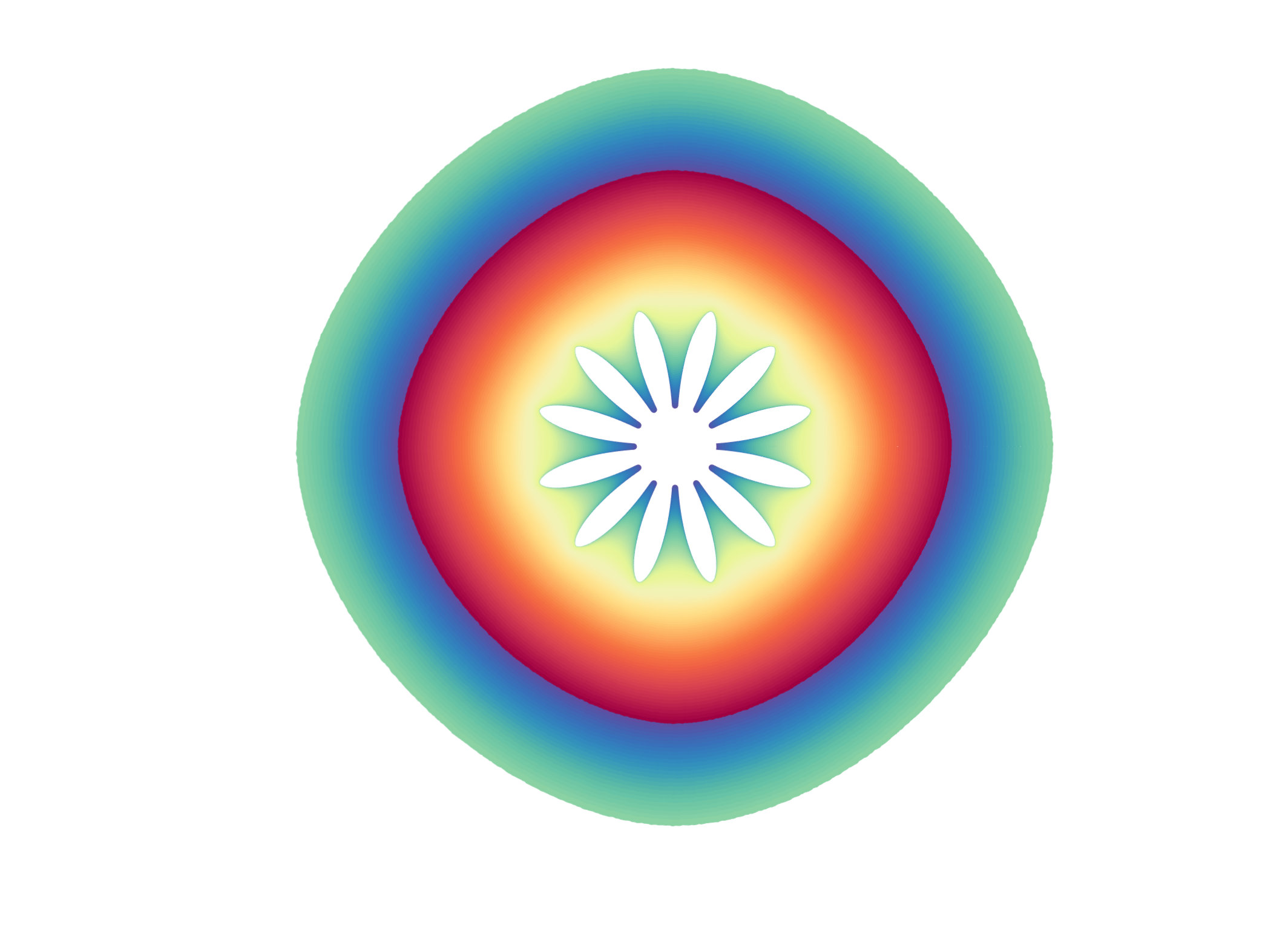 Figure 1
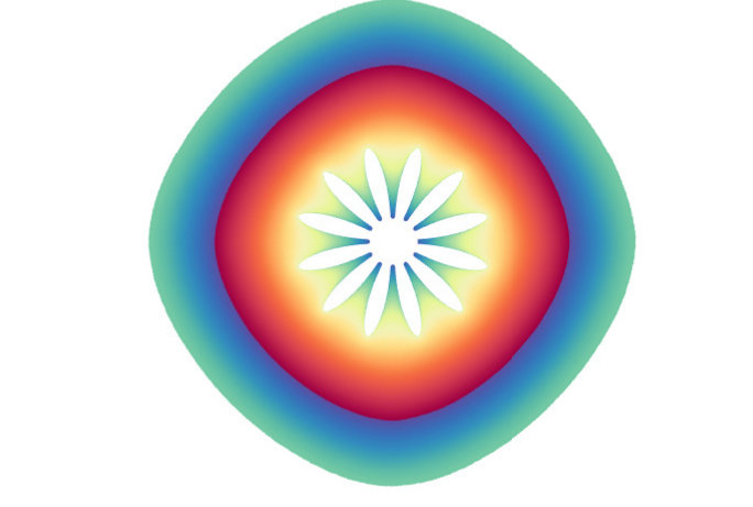 Figure 2
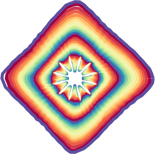 Figure 3
 Figure 4
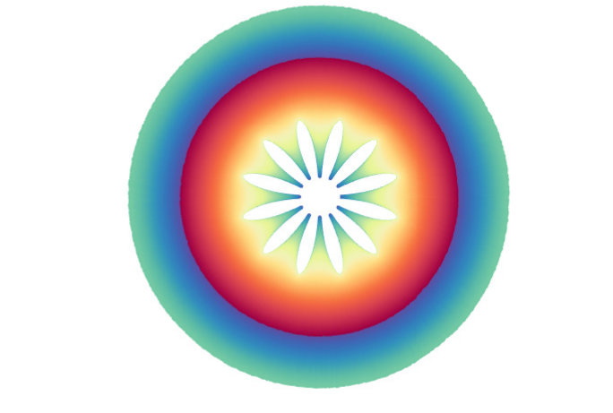 Figure 5
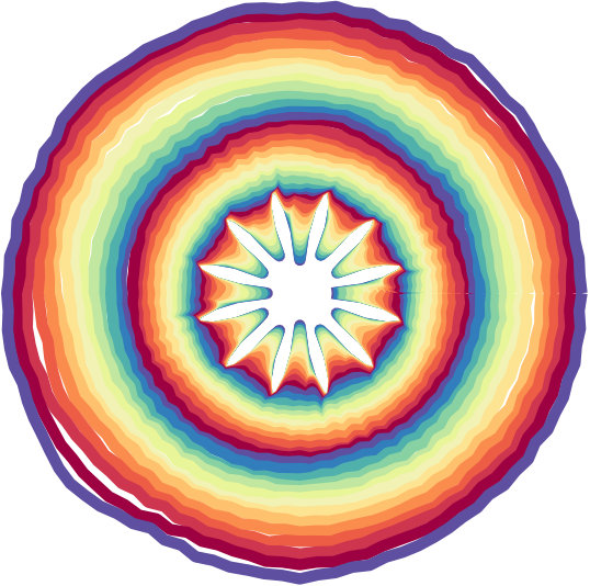 Figure 6
 Figure 7
 Figure 8
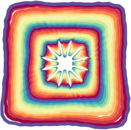 Figure 9
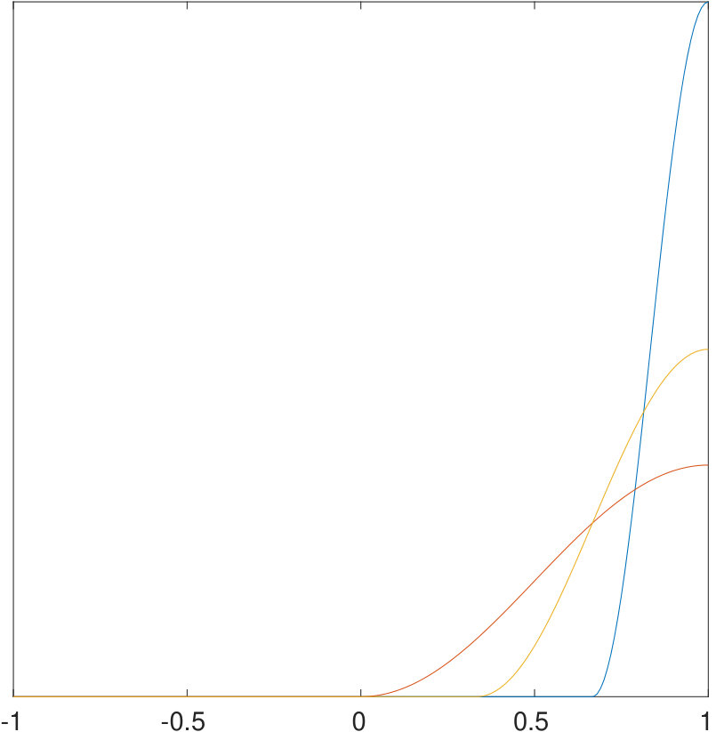 Figure 10
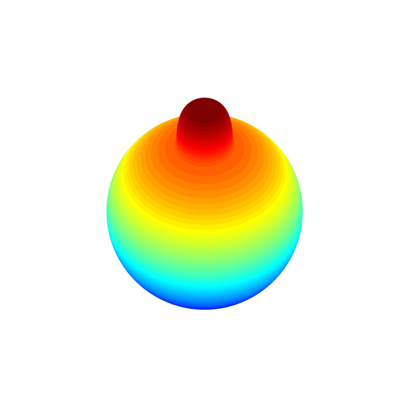 Figure 11
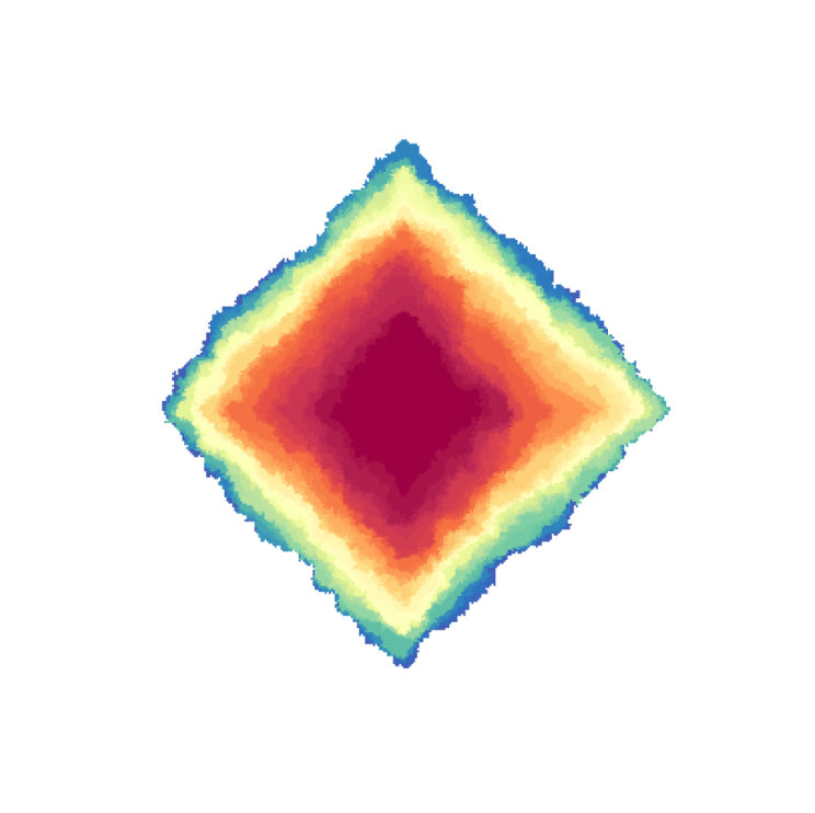 Figure 12
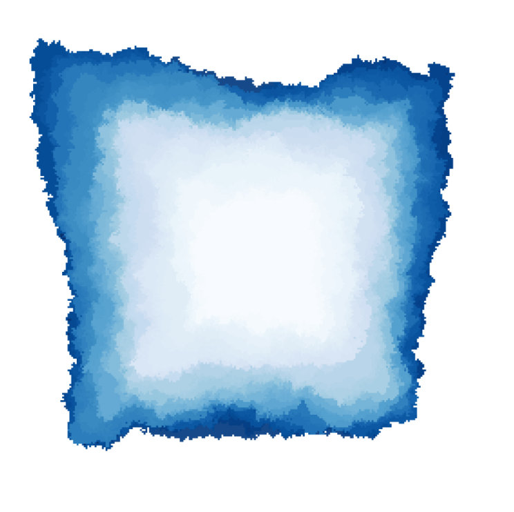 Figure 13
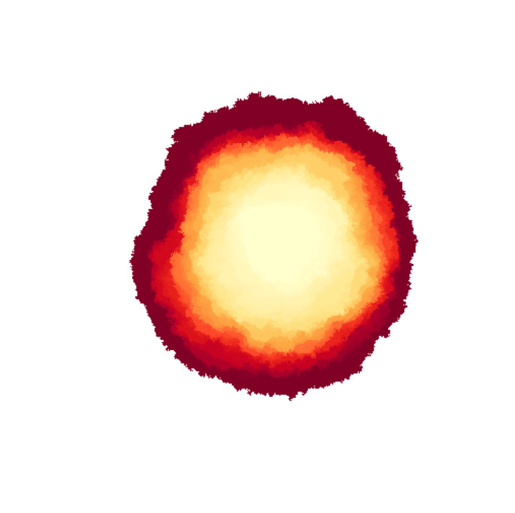 Figure 14
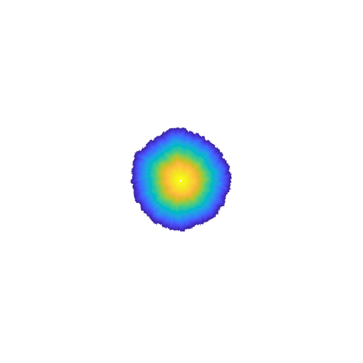 Figure 15
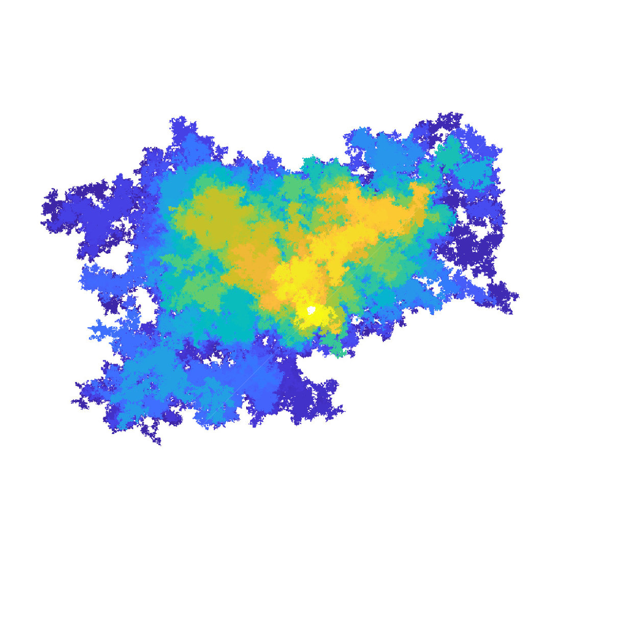 Figure 16
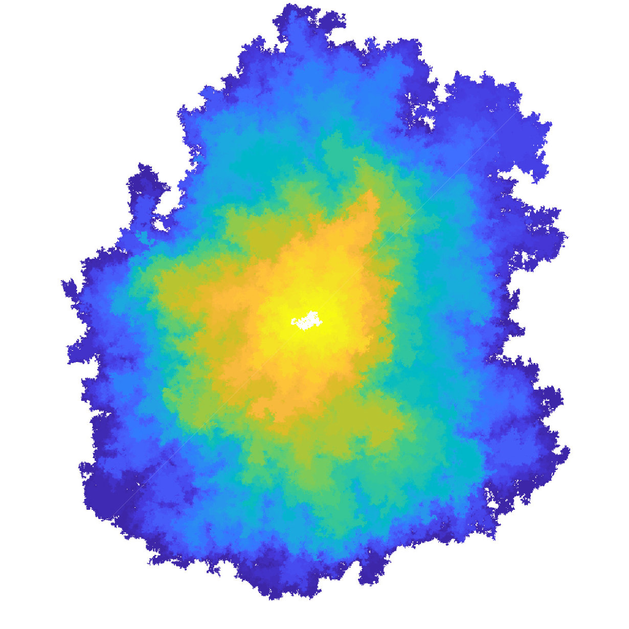 Figure 17
Peer Reviews
No public reviews on file for this paper yet. If you reviewed it on a platform where reviews are public (OpenReview, ICLR, NeurIPS, ICML), you can paste yours below so the community can read it here.
Videos
No videos yet. Explain this paper in a talk, walkthrough, or lecture? Add one.
Averaging principle and shape theorem
for a growth model with memory
Amir Dembo
Department of Mathematics, Stanford University.
,
Pablo Groisman
Departamento de Matemática, FCEN, Universidad de Buenos Aires, IMAS-CONICET and NYU-ECNU Institute of Mathematical Sciences at NYU Shanghai.
,
Ruojun Huang
Courant Institute.
and
Vladas Sidoravicius
Courant Institute and NYU-ECNU Institute of Mathematical Sciences at NYU Shanghai.
V. S. passed away in May 2019. The other authors dedicate this paper to his memory.
Abstract.
We present a general approach to study a class of random growth models in -dimensional Euclidean space. These models are designed to capture basic growth features which are expected to manifest at the mesoscopic level for several classical self-interacting processes originally defined at the microscopic scale. It includes once-reinforced random walk with strong reinforcement, origin-excited random walk, and few others, for which the set of visited vertices is expected to form a “limiting shape”. We prove an averaging principle that leads to such a shape theorem. The limiting shape can be computed in terms of the invariant measure of an associated Markov chain.
Key words and phrases:
Averaging principle, hydrodynamic limit, excited random walk, shape theorem.
2010 Mathematics Subject Classification:
60K35, 60K37, 82C22, 82C24
This research was supported in part by NSF grant DMS-1613091, UBACYT grant 20020160100147BA and PICT 2015-3154.
1. Introduction
Random growth processes arise in great variety in a large class of physical and biological phenomena, network dynamics, etc. Starting from seminal works of Eden [14] and Hammersley and Welsh [18], a series of mathematical models have been developed to capture and understand the evolution and pattern formation of growth processes. Our motivation stems from Laplacian growth models, which are characterized by the fact that the rate at which each portion of the boundary of the domain grows is determined by the harmonic measure of the domain from some given point, which we call source. The list includes Diffusion Limited Aggregation (dla) [40], its generalization – Dielectric Breakdown Model (dbm) [33], Hastings-Levitov process [21]; Internal dla (idla) [13, 29], abelian sandpiles and rotor aggregation [31]. It also includes once-reinforced random walk with strong reinforcement (orrw) [11], and origin-excited random walk (oerw) [28], for which the set of visited vertices is expected to form a limiting shape. For models such as dla, dbm or Hastings-Levitov, the source is at infinity, while in models such as idla, the source is at the origin. Whenever the source is fixed, the process of growing in time domains is Markovian. In contrast, the latter process is non-Markovian in orrw or excited random walks, where the source is moving and depends strongly on the last hitting point of the boundary and current shape of the domain.
In general, lattice growth models of this type are elusive, specially when the source is at infinity or when it is not fixed. A notable exception is idla for which Lawler, Bramson and Griffeath obtained a shape theorem (see [29]). Specifically, here particles are emitted in steps, one by one, from the source which is always located at the origin, and perform simple random walk until they visit an unvisited vertex. Each particle waits at the source until the previous one hits the external boundary, before being emitted. Gravner-Quastel [16] and Levine-Peres [30] generalize [29] and relate idla under more general, albeit still fixed, source locations to pde free boundary problems (a Stefan problem in [16], and an obstacle problem in [30] who also obtain analogous shape theorems for rotor-router and divisible sandpile models). An interesting variant is the Uniform idla, where upon hitting the boundary, the particle (source) is moved at a point chosen at random uniformly in the domain, and it is shown in [2] that the limiting shape of Uniform idla is the Euclidean ball.
Beyond these two examples, there is little understanding of such growth processes, despite substantial recent advances for first passage percolation. In particular, it is conjectured that for both orrw and oerw the evolution leads to the formation of an asymptotic shape as time goes to infinity (see [27, 28]), but there is no clear vision on how to attack the problem. Recall that in orrw the particle performs random walk on , but each edge (or vertex) increases its conductance by a fixed strength after the first time it is traversed. A phase transition is expected in terms of , with a limiting shape conjectured for all large enough. In the oerw model, the particle receives a (one-time) small drift towards the origin whenever it reaches an unvisited vertex (instead of the conductance change of the orrw), and a shape theorem is conjectured to hold, no matter how small this positive drift is. We refer the reader to [3, 26] for background on excited random walks, and to [2, 28] for discussions on various idla type processes and reinforced walks, all of whom share certain similar features. In particular, heuristically, whenever the self-interaction tends to attract the walker towards the bulk of its existing range, the boundary of the latter should change at a much slower rate than that of the walker, providing a natural setting to witness averaging.
While non-lattice isotropic models are more amenable to rigorous analysis (see [23, 34]), this typically requires having random conformal maps, hence restricted to dimension . By focusing instead on the evolutions of star-shaped domains in , we are able to handle any , and mention in passing that, on the deterministic side, the works [5, 6] are close in spirit to our averaged equation (1.12).
We consider here a general random growth model in which is specified by two rules , and a scaling parameter . The rule , which is allowed to depend on the whole geometry of the domain and the position of the source, determines the (random) point at the boundary where the particle, upon starting at the prescribed position, called source, is going to hit the boundary of the domain. For example, may be the Harmonic measure at the boundary of the domain from the source. After the particle hits the boundary, the domain grows around the hitting point with a volume increase of , followed by the particle jumping to the next source position, according to the rule .
More precisely, fixing a small parameter , we consider evolving domains in , which form simply-connected star-shaped compact sets (i.e. they can be parametrized by a function defined on the sphere ). It is a pure jump Markov process that starts with an initial domain and particle position and evolves at a Poisson rate of by increasing the domain around randomly chosen boundary points (or equivalently, spherical angles ). The probability density for choosing boundary points to evolve is given by the hitting kernel , which is a probability density on the sphere . After each hitting at the boundary at a point , the particle is instantaneously transported according to the specified rule to a point in that can depend on both the domain and the last hitting position. Contrary to the rule , we note that is deterministic in this article. In principle, one can consider a more comprehensive model where is a probability density function on , representing random transportation of the particle after each hitting of the current domain boundary.
The process of evolving domains in together with the position of the driving particle coupled to the former is, by construction, Markov (though each marginal is in general non-Markovian). The aim is to construct a continuum simplified model of “random walk interacting with its range”, allowing for general hitting kernel and non-trivial redistribution after each interaction, while inferring whether the evolving domain has an asymptotic shape.
The averaging principle has been extensively studied in the theory of dynamical systems, see e.g. [4, 7, 15, 20, 24, 35, 39] and references therein. Usually one identifies a slow variable and a fast variable. Under suitable conditions the fast variable achieves equilibrium in a time scale for which the slow variable does not evolve macroscopically. Hence, as the scale parameter one expects the slow variable to move according to a system where the fast variable is integrated with respect to its invariant measure, which may depend on the slow variable as well. In our model, the averaging property that one expects in models such as orrw and oerw is explicitly shown in terms of the process , where as , the variable serves as the slow variable, while acts as the fast one (and though the literature on averaging is large, we found no averaging principle that fits our case, involving a Markov jump process in infinite dimensions). The averaging principle is close in spirit to hydrodynamic limits, a standard tool in the study of interacting particle systems (see [12, 25, 38] and references therein). A hydrodynamic limit is proved for a continuous version of idla in [16], yielding in turn a shape theorem, thanks to the scale invariance of this model (as in Lemma 3.1 below). As mentioned before, in this process particles are emitted from fixed sources. One of our goals here is to derive similar results for self-interacting random walks, where the source is clearly moving.
Under certain mild conditions on our model features (namely, the rules and ), we prove in Theorem 1.4 an averaging principle. It allows us to identify the limiting infinite-dimensional ode governing the evolving domain as the slower dynamics of the pair, yielding in Theorem 1.9 the limiting shape result as a stationary solution of the limiting ode. Then, in Theorem 1.10 we verify our assumptions for a certain class of models, and in some instances compute explicitly their limiting shape.
Let be the unit sphere in equipped with its Euclidean surface area measure and for any let denote the norm of with respect to . We denote by the space of strictly positive continuous functions on .
Definition 1.1**.**
A simply-connected compact set is called star-shaped with respect to , if the line segment connecting [math] and any is entirely contained in .
Any star-shaped is uniquely represented by a non-negative function as
[TABLE]
Hereafter, by a slight abuse of notation, we identify any with its graph, which encloses a star-shaped domain and denote by the Lebesgue measure (or volume) of that domain . Namely,
[TABLE]
Let be an open subset of such that is non-empty for any . The measurable map
[TABLE]
assigns to each a strictly positive, continuous probability density function with respect to . This function represents the rule whereby a particle starting from chooses a point , at the boundary of the domain enclosed by , to be the center of the (small) bump we add on the domain boundary . The measurable map
[TABLE]
assigns for each and the transported (source) location of a particle that hits the domain boundary at angle . Assuming that for any and -a.e. , guarantees that a.s. the iterative composition of the rules and is well defined (per our dynamics (1.7)). The small bump we add is in the form of a suitable spherical approximate identity , as defined next.
Definition 1.2**.**
A collection of continuous functions is called a spherical approximate identity if , and as , for every , where (see [9, (2.1.1)]),
[TABLE]
is the surface area of , and denotes the scalar product associated with the Euclidean norm in . We call such collection local if in addition is supported on the spherical cap of (Euclidean) radius centered at and are uniformly bounded.
Utilizing [9, Section 2.1] we characterize in Lemma A.1 the collections that form a local spherical approximate identity (see also Figure 3).
Throughout we set the positive function on ,
[TABLE]
Noting that for of density
[TABLE]
(c.f. proof of Proposition 1.7), we add at each update a bump on the current boundary , where is a local spherical approximate identity, so that for , the volume of should grow at a nearly constant, unit rate. Using the -dependent
[TABLE]
as our spherical-scale parameter yields a bump on the boundary of about height (in the radial direction), uniformly in , which is supported in case of a Euclidean ball of unit surface area (namely, ), on spherical caps of radius . Clearly, when adding such -dependent bumps to our boundary function, the star-shaped domain evolves by a localized bump and the new domain remains star-shaped. Specifically, fixing and starting at some we construct the Markov jump process of jump rate and state space , as follows. For a sequence of auxiliary Poisson arrival times of rate , starting at , we freeze during each of the intervals , while as each , , conditional on the canonical filtration
[TABLE]
let
[TABLE]
That is, given the random has the density with respect to . Then, update according to
[TABLE]
(recall the definitions (1.2) of and (1.4) of ).
The generator of the Markov process is
[TABLE]
for any in the domain of . For and let
[TABLE]
Considering (1.8) for the evaluation map at fixed and using (1.1), we get for the decomposition
[TABLE]
where is an -martingale. Similarly, taking , , in (1.8) yields
[TABLE]
for some -valued, -martingale . For let denote the -valued Markov jump process evolving by (1.10) in the frozen domain . Its generator is thus
[TABLE]
for a suitable collection of functions . Consider also the deterministic dynamics given by
[TABLE]
The probability measures on for will be specified in Assumption (E), with Proposition 1.6 establishing the existence and uniqueness of the solution for the infinite-dimensional ode (1.12). For every and , we define the collections
[TABLE]
and assume the following Lipschitz properties of , and throughout .
Assumption** (L).**
For any , there exists finite such that uniformly for , , we have that
[TABLE]
Moreover, for any ,
[TABLE]
Our other two assumptions concern the ergodicity of the particle process in a frozen domain and the convergence to of the drift of when .
Assumption** (E).**
For any the process of generator (1.11) has a unique invariant probability measure , such that
[TABLE]
where as , for any fixed .
Assumption** (C).**
For the -stopping times
[TABLE]
any fixed and ,
[TABLE]
Remark 1.3**.**
From Definition 1.2 we know that as , for any fixed . For Assumption (C) we need this to hold at the -dependent , but see parts (c) and (d) of Proposition 1.6 for simple sufficient conditions for Assumptions (E) and (C), respectively.
Equipped with these assumptions, we next state our main result. For technical reasons, we need to introduce a stopping time giving a lower bound to , as needed to apply the crucial Lemma 2.1.
Theorem 1.4** (Averaging principle).**
Under Assumptions (L), (E) and (C), starting at , for the -stopping time
[TABLE]
and any , , we have that for any
[TABLE]
where denotes the unique -solution of the ode (1.12) starting at (see Proposition 1.6(b)).
Remark 1.5**.**
With minor modifications of the proof, we can accommodate in Theorem 1.4 any random initial data such that in probability. It is crucial to have strictly positive, since the function blows up when , hence (1.15) fails near . Of course, if for any ,
[TABLE]
then we can dispense with the stopping time in (1.21).
The next proposition, whose proof is deferred to the appendix, clarifies the implications of our assumptions.
Proposition 1.6**.**
(a) If condition (1.13) of Assumption (L) holds, then for every there exists such that for all ,
[TABLE]
Similarly, if (1.13) holds with , then the same applies for (1.23).
Further, conditions (1.13) and (1.14) imply that for all ,
[TABLE]
*while if (1.13) holds for both and , with (1.14), (1.16) and (1.22) holding as well, then (1.15) must also hold.
(b) Condition (1.15) at , together with Condition (1.16) imply that starting at any the ode (1.12) admits a unique -solution on . Further, up to time the solution of (1.12) is in for some .
(c) To verify Assumption (E), it suffices to show that for any there exist and , such that the jump transition probability measure of the embedded Markov chain satisfies the uniform minorisation condition*
[TABLE]
*for any and some probability measure on .
(d) Assumption (C) holds if for any ,*
[TABLE]
(e) Condition (1.16) implies that for some positive and any
[TABLE]
with the -stopping times of (1.18) and
[TABLE]
Recall (1.3) that the random dynamics (1.6) has expected volume increase of at each Poisson jump, (irrespective of the precise choice of as ). We thus expect the following result (whose proof is also deferred to the appendix), about the linear growth of the volume of the deterministic dynamics (1.12).
Proposition 1.7**.**
If the solution to the ode (1.12) belongs to for all , then . Further, (1.3) holds throughout .
Under the following scaling invariance of and , we will deduce a shape theorem for the process , from the averaging principle of Theorem 1.4.
Assumption** (I).**
For any scalar , if then and
[TABLE]
Definition 1.8**.**
(a) A function is called invariant (shape) for the ode (1.12), if starting at yields
[TABLE]
(b) A function is called attractive (shape) for the ode (1.12) and a collection of initial data, if starting at any , the solution exists, with
[TABLE]
In general, invariant shapes may not be unique, nor are they necessarily attractive. See Example 3.4.
Theorem 1.9** (Shape theorem).**
*Suppose Assumption (I) holds and (1.21) applies without the stopping time (see Remark 1.5).
(a) If a function with is invariant for the ode (1.12), then for any , and ,*
[TABLE]
*(b) If a function with is attractive for the ode (1.12) and a collection of initial data, then for any and , *
[TABLE]
Our main application is a model of random growth on motivated by the expected mesoscopic behavior of orrw and oerw on , where to gain regularity we consider and defined via a smoothed version of the evolving domain. Specifically, fix and as in (A.14) for some . Then, for every (see (1.1)). We set
[TABLE]
where denotes the Green’s function of the Laplacian on star-shaped domain with Dirichlet boundary conditions at and is the inward normal derivative on . Similarly, fix a locally Lipschitz function such that
[TABLE]
and set (see Section 4 for the probabilistic interpretation),
[TABLE]
Another natural hitting rule chooses a boundary point with probability “proportional to a function of the distance to the particle”. Specifically, fixing a locally Lipschitz and with as above, replace (1.32) by
[TABLE]
while keeping the rule of (1.34). We have the following results for these rules.
Theorem 1.10**.**
(a) The Averaging Principle of Theorem 1.4 holds under either (1.32)-(1.34) or (1.33)–(1.35), without the stopping times of (1.20).
(b) In case and , the Shape Theorem 1.9 also holds. In particular, for with fixed, the centered Euclidean ball is an invariant shape.
(c) For , and setting in (1.32) and (1.35), the centered Euclidean ball is uniquely attractive among initial data.*
Remark 1.11**.**
Similar conclusions apply for other transportation rules, such as
[TABLE]
which sends the particle to a statistical center of the domain. Note that may possibly be outside the domain, and if start-shaped is invariant for the ode corresponding to (1.36) and (1.32), then so are all translations of which are star-shaped. Also, for such which depends on the domain only, trivially the invariant measure is the Dirac mass at and Assumption (E) holds.
The rest of the article is organized as follows. In Section 2 we prove Theorem 1.4 and in Section 3 we deduce the shape result, Theorem 1.9. In Section 4 we apply these theorems to concrete growth models and prove Theorem 1.10.
2. Proof of Theorem 1.4
We start with bounding the Wasserstein 2-distance between any two measures on a compact, connected Riemannian manifold, by the -distance between their densities with respect to the Riemannian measure.
Lemma 2.1**.**
Let be a connected Riemannian manifold without boundary compactly embedded in , equipped with its Riemannian distance and measure . Let be probability distributions on having densities respectively with respect to , where in addition for all . Then, there exists such that
[TABLE]
where
[TABLE]
is the Wasserstein -distance between and , and .
Proof of Lemma 2.1. .
By [36, Theorem 1], we have the variational representation
[TABLE]
In the last step, we have used the Poincaré inequality , where denotes the -weighted average of in and is the Poincaré constant. ∎
The proof of Theorem 1.4 is based on considering an auxiliary process in which the slow variable is frozen (this is a standard tool for proving averaging principles, see [20, 39]). Set
[TABLE]
Given the main process , we consider a family (indexed by ) of auxiliary dynamics defined piecewise on each time interval with , on the same probability space as the main process, as follows. Inductively for every , take the same Poisson clock used in constructing the main process, and starting at , let have the marginal distribution of the Markov jump process in the frozen domain defined as in (1.11). That is, jumps at each , in the frozen domain , by first using probability density to choose a spherical angle , then applying the rule . We further put requirement on the joint law such that at each jump, and of (1.5) achieve within twice the Wasserstein -distance on , where , . Inductively the above procedure defines on .
We then define on as the dynamics driven by the ode, with ,
[TABLE]
With the auxiliary processes in place, we proceed to the proof of the theorem. By Proposition 1.6(b), starting at , the solution to the ode (1.12) exists and is unique in . Fixing , since , for any the stopped at of (1.18), sample path remains within , provided . Hereafter, we only apply Assumptions (L) and (E) with Lipschitz constant , resp. convergence rate in (1.17), depending on such fixed , for the stopped processes.
Next, by (1.9), for any we have per ,
[TABLE]
By [10, Proposition 8.7], for the stopped martingale ,
[TABLE]
which together with Fubini, implies that
[TABLE]
Further, since spherical convolution is a contraction in (per Definition 1.2), and the Lipschitz bound (1.23) holds throughout , hence the norms are uniformly bounded,
[TABLE]
for some finite and all . Consequently, by (2.3)-(2.5) and Cauchy-Schwarz, for any ,
[TABLE]
We let hereafter (for and of (1.18) and (1.20), respectively), and rely on (2) to establish the following two lemmas.
Lemma 2.2**.**
In the setting of Theorem 1.4, we have that
[TABLE]
Lemma 2.3**.**
In the setting of Theorem 1.4, we have that
[TABLE]
While deferring the proofs of Lemmas 2.2 and 2.3 to the end of the section, we note that these lemmas together with the definition (1.27) of yield that
[TABLE]
In view of Proposition 1.6(d), this in turn results with
[TABLE]
(provided ). The conclusions of Lemma 2.2 and Lemma 2.3 are thus strengthened to apply with instead of , so combining these lemmas with Markov’s inequality completes the proof of the theorem.
Turning to establish Lemmas 2.2 and 2.3, we start with the following key bound.
Lemma 2.4**.**
In the setting of Theorem 1.4, for some finite we have
[TABLE]
Proof of Lemma 2.4. .
Per (1.11), for each the auxiliary process admits the decomposition
[TABLE]
for some -valued, -martingale (setting when ). Taking the difference of (2.10) with (1.10), we have that for ,
[TABLE]
is an -valued martingale.
Considering the generator of , we have by [10, Proposition 8.7] and (1.14) that for any ,
[TABLE]
where the inner conditional expectation is only over , having marginal densities and , with respect to on . By the coupling we chose, and Lemma 2.1 with , bounded below by when , we have in (2) for ,
[TABLE]
using (1.13) in the last line. Consequently, we obtain from (2) that
[TABLE]
using in the last line (2) and that . From (2.11) at , Cauchy-Schwarz inequality, (2), (2) and , we have that for some finite and any , ,
[TABLE]
utilizing also that is Lipschitz, as in (1.24) of Proposition 1.6(a). By Gronwall’s inequality for , starting at , we get that
[TABLE]
For our choice (2.1) of , the rhs of (2.14) is bounded by for some (other) finite , as claimed. ∎
Proof of Lemma 2.2. .
Per (1.9) and (2.2), for any we have that
[TABLE]
Consequently, by Cauchy-Schwartz,
[TABLE]
where the first term tends to zero as by Assumption (C) and the uniform boundedness of the integrand. The remaining two terms are bounded via (1.23), (2)-(2) and Lemma 2.4 by
[TABLE]
for some generic constants , hence tending to zero as well. ∎
Proof of Lemma 2.3. .
Per (1.17) and the fact that the event is measurable on , we have that uniformly for ,
[TABLE]
It then follows from (2), (1.15) and (2) that for some finite and any ,
[TABLE]
where as by (1.17) since . We proceed to bound
[TABLE]
via Gronwall’s inequality. Per (2.2) and (1.12), for any we have that
[TABLE]
By (1.15) and (2) we have that for any ,
[TABLE]
Gronwall’s inequality and Lemma 2.2 yield that
[TABLE]
converge to zero when , as required. ∎
3. Proof of Theorem 1.9.
The following intuitive coupling enables to transfer the Averaging Principle for the family of processes as the scale parameter on finite time horizons, into a shape result for of scale as time .
Lemma 3.1** (coupling).**
Fix . Under Assumption (I), with
[TABLE]
there exists a coupling such that
[TABLE]
Proof.
Let with denote the sequence of Poisson jump times of rate used in constructing , for some fixed . Set , . By scaling properties of exponential distribution, has the law of a sequence of Poisson arrival times of rate , as such we construct using , on the same probability space as .
Starting with on , suppose we have succeeded in coupling with as in (3.1) up to time for some . Then by (1.28), for any we have
[TABLE]
The induction hypotheses and the construction (1.5), (1.6) yield at , per
[TABLE]
By coupling the jumps of and at such that , we deduce , for , and by (1.7), (1.29) also . During , all processes stay put, hence continuing extends the coupling to all . ∎
Proof of Theorem 1.9..
We only prove part (b), whereas the proof of part (a) is similar. By Theorem 1.4 and Lemma 3.1, we firstly have for any and ,
[TABLE]
where is the continuous solution of (1.12) with initial data , and . By the triangle inequality, we have that
[TABLE]
By (3.2), the first term vanishes for any , and upon taking another limit as , the second term vanishes as well by (1.30). We obtain the claims upon setting . ∎
Problem 3.2**.**
It remains open to remove the strict positivity of initial condition in Theorem 1.4, hence to be able to take in (1.31), which would correspond to a genuine shape theorem.
We have the following general characterization of invariant shapes.
Proposition 3.3**.**
Under Assumption (I), is invariant for the ode (1.12) if and only if .
Proof.
We prove the “only if” part, while the converse “if” direction can be checked directly. Assumption (I) implies that for any , and hence . From (1.11) the value of is independent of . The natural coupling implies that of Assumption (E) are merely the push-back of under scaling , resulting with . Per Definition 1.8(a), an invariant solution starting at is such that with . From the ode (1.12) it is not hard to infer that . Further, by taking derivative of (1.12) in we identify the proportionality constant to be . ∎
However, invariant shapes may not be unique.
Example 3.4**.**
Consider (the origin) and . Then it is easy to check that
[TABLE]
Since this choice of and satisfies Assumption (I), by Proposition 3.3, any is invariant for (1.12), and not attractive except when starting from itself.
We provide sufficient condition for the centered Euclidean ball to be attractive for (1.12), where we denote henceforth by the constant function on . Unfortunately, the condition (3.3) is rather hard to check.
Proposition 3.5**.**
Suppose the ode (1.12) has -solution for any , and that for any , it holds
[TABLE]
Then is attractive for (1.12) for the collection of initial data.
Proof.
Set . Since is for all , we have
[TABLE]
and similarly for . Therefore, combined with (3.3) we have that
[TABLE]
Set . Then we have that and
[TABLE]
This yields
[TABLE]
as , for any . Equivalently, for some constant such that ,
[TABLE]
This is exactly the definition (1.30) of attractive shapes with . ∎
4. Applications: Proof of Theorem 1.10
We consider the two applications of Theorems 1.4 and 1.9, introduced previously in Theorem 1.10, with the main one being a simplified model for the growth of the range of oerw (with the density of the harmonic measure). Indeed, our choice of (1.34) is motivated by basic features of orrw and oerw in the mesoscopic scale. The ideal choice of to be closer to these models would be , with (1.34) an independent of , rule of the same type. Similarly, our choice of for (1.32) corresponds to taking a simplified continuous model, where the random walk is replaced by a Brownian motion (see the probabilistic interpretation provided in Section 4.1). An advantage of using such continuous model is that our proofs work verbatim when instead of Brownian motion, the particle follows an elliptic diffusion whose generator is a uniformly elliptic second-order divergence form operator (so the Green’s function used in the definition (1.32) be the one for ). Indeed, recall Dahlberg’s theorem [8, Theorem 3 and remark], that for a Lipschitz domain , harmonic measures from any point are mutually absolutely continuous with respect to the -dimensional Hausdorff measure on , hence their Radon-Nikodym derivative which is the Poisson kernel exists and belongs to . If the domain is more regular, so is the Poisson kernel. Per [22, page 547], if belongs to Hölder space for some , then . Since our domains are star-shaped, by an abuse of terminology we will call the Poisson kernel of , if it is a probability density on corresponding to with up to a change of variables.
As for the reasoning behind the regularization in our applications, note that even for smooth domains, one cannot expect their Poisson kernel to be Lipschitz in -norm with respect to boundary perturbations as (1.13), or in any other norm. Indeed, as explained in [22], one expects the regularity of to be one derivative order less than that of the domain . However, if one forms the kernel based on a regularized domain, then the Lipschitz property can be true (as shown below in Proposition 4.3). Though to a lesser degree, similar issue arises also in the more explicit hitting rule of (1.35), where regularization is still the key to verifying Assumption (C) via condition (1.26).
Recall the and , norms of functions, taking in this article only or (the closure of a bounded domain ), and using for . Letting for multi-index denote any -th order derivative of , we equip the collection of -times continuously differentiable functions, with the norm
[TABLE]
Further denoting the -Hölder semi-norm of a function by
[TABLE]
if finite, where is the geodesic distance when , and the Euclidean distance when , we define the -Hölder norm of any , by
[TABLE]
We proceed to verify the conditions needed for Theorems 1.4 and 1.9, starting with the following Lipschitz control on the regularization map , the proof of which is deferred to the appendix.
Lemma 4.1**.**
For any , we have that
[TABLE]
for some that depends only on the convolution kernel . In particular, for any there exists so the image of under is within the set
[TABLE]
where denotes the open Euclidean ball of radius centered at and denotes the domain of boundary .
Equipped with Lemma 4.1, we prove property (1.14) for of (1.34).
Proposition 4.2**.**
For every , the map is Lipschitz from to .
Proof.
With Lipschitz on compacts, we have by Lemma 4.1 that for of (1.34), some finite and all ,
[TABLE]
Also, for any , ,
[TABLE]
The uniform on control from Lemma 4.1, translates into the same control over the bounded Lipschitz norm of . Hence, with Lipschitz on compacts, we deduce that for some finite and all as above. ∎
4.1. Smoothed harmonic measure
Recall the construction above (1.32) of the smoothed domain for every . Due to the preceding discussion on Poisson kernels, it is clear that the regularized (as in (1.32)) Poisson kernel belongs to for any , where the probabilistic meaning of the definitions of in (1.32) and in (1.34) is as follows.
If the process is defined up to time and the state at that time is given by domain with boundary and particle position , we wait for the next jump mark, denoted by , and given by an independent Exponential() random variable. To choose a point at the current boundary , the particle follows the law of a Brownian motion in , starting at till its first exit from the smoothed domain . We record its exit angle and define the location for the center of the new bump on the original domain by . Hence the updated domain is formed by
[TABLE]
Observe that the bump is added to the original domain and not the smoothed one. Next, the particle is pushed towards the origin by a strictly positive quantity, along the radius, still in the smoothed domain , namely and there it waits for the next jump mark. Continuing in this way we define the process at all times. Note that we have omitted the travel time of the Brownian motion inside the smoothed domain and only deal with its exit distribution. Further, since , for all , necessarily also , with the particle always contained in the smoothed domain, once we assume it is the case for .
We postpone to the appendix the proof of the following key proposition about Lipschitz regularity for Poisson kernels in our regularized domains (where the precise value of is unimportant).
Proposition 4.3**.**
For any , , , the map of (1.32) is Lipschitz from the set of (4.2), equipped with the -norm for the first variable and the Euclidean norm for the second one, to .
The map of (1.32) is a composition of and . The former map is globally Lipschitz per Lemma 4.1, whereas the latter is per Proposition 4.3 globally Lipschitz on some that contains the image of under the first map, yielding the following corollary.
Corollary 4.4**.**
For every , the map is globally Lipschitz from to .
Remark 4.5**.**
From Corollary 4.4 we get that for all , hence Assumption (C) holds in our setting (see Proposition 1.6(d)).
We next show that of (1.32) is bounded above and below, uniformly in , thereby verifying (1.16) and as explained in Remark 1.5, allowing us also to dispense of the stopping time in Theorem 1.4.
Proposition 4.6**.**
For each there exist such that
[TABLE]
Proof.
For each , the state space of is contained in the star-shaped domain enclosed by . In such domains, with in the interior, the Poisson kernel is pointwise positive (a consequence of Hopf lemma). By Proposition 4.3, is continuous per fixed with continuous per fixed . Thanks to the compactness of , the joint continuity of follows and we get (4.3) from Lemma 4.1 and the compactness of under the norm (see proof of Proposition 4.3). ∎
Remark 4.7**.**
Propostion 4.6 further establishes Assumption (E) for our model. Indeed, the sufficient condition (1.25) of Proposition 1.6(c), then holds with , and the push-forward under of the uniform measure on .
Remark 4.8**.**
With , hence also , Corollary 4.4 implies that (1.13) holds for both and . Recall Proposition 4.2 that (1.14) holds here, and Proposition 4.6 that so do both (1.16) and (1.22). Combined, these in turn yield by Proposition 1.6(a) the last remaining Lipschitz condition required (namely, property (1.15) of ), and thereby complete the verification of Assumption (L) in our setting.
Having verified Assumptions (C), (E) and (L) (see Remarks 4.5, 4.7 and 4.8, respectively), we can apply Theorem 1.4 to this model without the stopping time of (1.20). This amounts to proving Theorem 1.10(a) for this model, whereas our next proposition, considering special cases where we have explicit descriptions, constitutes the proof of Theorem 1.10(b) in this setting.
Proposition 4.9**.**
(a) If the function does not separately depend on , then the centered Euclidean ball is an invariant solution to (1.12).
(b) If the function depends linearly on , then Assumption (I) is satisfied.
(c) If for some fixed number , then the unique invariant measure is explicitly given by the harmonic measure from the origin in the domain enclosed by , for every .
(d) If and we force , then is the unique attractive solution of (1.12), whenever .*
Proof.
(a). First note that , so regularization by has no effect here. Further, by the rotational invariance of the Brownian law, the uniform measure on is invariant for the process (i.e. a Brownian motion on starting at and radially projected back to that set upon hitting ). In addition, recall (1.2) that is constant, hence so is , from which it directly follows that is invariant for (1.12).
(b). The identity (1.28) is due to the scaling invariance of the Brownian motion, while (1.29) is satisfied by our choice.
(c). By the scaling invariance of Brownian motion, the harmonic measure from the origin on and on , viewed as measures on spherical angles, are equal. Since the transition kernel of the Brownian motion from to is exactly given by , we see that the harmonic measure from the origin is the unique (thanks to Assumption (E)), invariant measure for .
(d). Since (the origin), here . By Corollary 4.4, . Hence, for any , the ode (1.12) admits solution . By Proposition 3.5, for to be attractive for (1.12) it suffices to show that for any , the Poisson kernel from the origin to , is at angle no smaller than at . To this end, upon forcing consider two standard Brownian motions in , one in the domain enclosed by , the other in the Euclidean ball . Couple them to move together starting from the origin until the first hitting time by both of , where one Brownian motion is stopped and the other can continue to move until hitting . This coupling yields that . An analogous coupling, between a Brownian motion in the domain enclosed by and another in , yields that , thus verifying our claim. ∎
For anisotropic (that do not satisfy the condition of Proposition 4.9(a)), one may obtain other limiting shapes as invariant solutions to the ode (1.12), such as diamond, square etc (see Figure 4), implicitly determined as in Proposition 3.3 (and in the anisotropic case, the Euclidean ball is typically not an invariant shape).
4.2. Distance to particle
Following the approach of Section 4.1, in particular as in Remarks 4.5, 4.7 and 4.8, our next proposition establishes Theorem 1.10(a) (namely, shows that Theorem 1.4 applies without of (1.20)), for of (1.35), where the probability of choosing a boundary point is a fixed function of its distance to the particle.
Proposition 4.10**.**
For every , the map of (1.35) is Lipschitz from to , for both and . In addition, is bounded, uniformly over , while is bounded above and away from zero, uniformly over .
Proof.
Starting with the boundedness above and away from zero of , we have in view of Lemma 4.1 that . The argument of in (1.35) is thus bounded, uniformly over . Now recall from Lemma 4.1 that for some and all , the point is at least away from , and thereby the argument of in (1.35) is bounded away from zero uniformly over . The uniform over bound above and away from zero on is then a direct consequence of our assumption that is positive and continuous on .
Next, with the numerator of (1.35) uniformly bounded above and the denominator uniformly bounded below, it suffices to separately prove the Lipschitz property for the numerator and denominator in (1.35). To this end, note that is globally Lipschitz on compact subsets of . Dealing simultaneously with and , it follows that for some finite and all ,
[TABLE]
where all -norms are with respect to . The difference between the denominator values at and is at most the -norm of the difference between the corresponding numerators, hence its Lipschitz property follows from the preceding bound.
Finally, note that is uniformly bounded on , hence the same applies for . With Lipschitz on compacts, it thus follows that is uniformly bounded on . ∎
We turn to get the analog of Proposition 4.9 for this model, thereby establishing Theorem 1.10(b) in this setting.
Proposition 4.11**.**
(a) If the function does not separately depend on , then the centered Euclidean ball is an invariant solution to (1.12).
(b) Assumption (I) holds whenever , for some .
(c) If , and we force , then is the unique attractive solution of (1.12), whenever .*
Proof.
(a). Following the proof of Proposition 4.9(a), the invariance of to a common rotation of yields that the uniform measure on is invariant for .
(b). It is easy to check that having in (1.35) results with (1.28) holding, whereas (1.29) is satisfied by the assumed linearity in of . Thus, Assumption (I) holds in this case and from part (a) we know that when the ball is an invariant solution to (1.12).
(c). For and , one has that
[TABLE]
In particular, for any , the ode (1.12) with of (4.4) admits solution and in view of Proposition 3.5, for to be attractive for (1.12) when , it suffices to have along such solution , the regularized no smaller at angle than at . This indeed holds once we force . ∎
Appendix A
Proof of Proposition 1.6.
(a) Since is a ratio of and the scalar , with on and assumed Lipschitz in -norm on this set (by (1.13)), it suffices to show that in addition is Lipschitz in that norm (on ). To this end, note that for any and ,
[TABLE]
by Hölder’s inequality and expanding . Considering either , or , , our claim follows from (1.13) at , since is non-decreasing for functions on .
Turning next to , for any , by (1.13), (1.14),
[TABLE]
as needed.
Fixing , and dealing simultaneously with and , we proceed to show that is Lipschitz from to . To this end note that the Markov chain on of transition kernel density with respect to the uniform measure, is, by (1.22), uniformly ergodic throughout , with ergodicity coefficient depending only on (via ), and as such, has a unique invariant measure on . Further, as the rule is non-random, the invariant measure of the Markov chain is merely the push-forward by of the aforementioned with of (1.12) represented alternatively as
[TABLE]
Next, recall the preceding where we saw that (1.13) results with (1.23) holding at the corresponding value of . Combining the latter with (1.14), we deduce that the analogous to (1.23), uniform over Lipschitz bounds, apply also for . Thus, utilizing the characterization of total variation norm of finite signed measures (cf. [17, page 124]), we have for some finite constant and all ,
[TABLE]
Turning to the first term, recall that throughout , so in view of (1.16) it suffices to bound . Denoting by the space of signed Borel measures on with total variation one, we find that (per notation in [32, (2.1)]), for some and ,
[TABLE]
(using in the above, also (1.13) and (1.14)). Consequently, by [32, Corollary 3.1], for some which depends on the uniform ergodicity coefficient,
[TABLE]
thereby completing the proof.
(b) Consider the Banach space , and the subset for some . Since per (1.15), the map is Lipschitz from to in , there exists a unique continuous solution to (1.12) locally in time, defined up to the first exit time of the set , cf. [1, Theorem 7.3]. Hence, Proposition 1.7 holds as long as the solution is defined, and we can bound the growth of its -norm by Hölder’s inequality
[TABLE]
This in turn implies the following bound on the growth of ,
[TABLE]
in terms of of (1.16), thereby leading to
[TABLE]
Thus, by the ode (1.12), as long as the solution is defined, we have control on the growth of its -norm,
[TABLE]
Given any , taking in the beginning , ensures the existence and uniqueness of a continuous solution up to time .
(c) The minorisation (1.25) implies by standard theory of general state space Markov chains (see [37, Theorem 8]), that for any the embedded chain has a unique invariant measure , with the uniform on convergence
[TABLE]
The proof is by coupling, which extends to the process with and its stationary version (i.e. starting at distribution and using the same jump times for both processes). It follows that the processes coalesce at the coupling time with
[TABLE]
for some positive constant , any and all . By the triangle inequality, employing this coupling for proving (1.17), we separately bound
[TABLE]
and
[TABLE]
There is no contribution to (A.1) from and a-priori for all . Hence (A.1) is at most . By stationarity the expectation in (A.2) is independent of and utilizing the Markov property, it equals
[TABLE]
where by Fubini
[TABLE]
Using the preceding coupling per value of in (A.3), we deduce that
[TABLE]
where by Cauchy-Schwarz, for the pre-compact ,
[TABLE]
Plugging into (A.3) this uniform bound on and the uniform tail bound on , bounds the term (A.2) by , thereby completing the proof.
(d) The processes are, for some , within , whereby . Thus, given (1.4), the definition of and the bound (A.21) on , it suffices for Assumption (C) to bound the rate of convergence to zero as , for the rhs of (A.21) at , uniformly over . In particular, recall from (A.18) that (since when ), hence (1.26) suffices for Assumption (C) to hold.
(e) By our construction and (1.4), any bump added to some is supported on a spherical cap in whose radius is at most
[TABLE]
Proceeding to cover by spherical caps of radius , in view of (A.4) the growth of somewhere within requires that hit the concentric cap of radius . Further, for of (1.27) and ,
[TABLE]
Thus, for any , the probability of hitting a spherical cap of radius , is by (1.16) and (A.5), at most . Consequently, the total number of changes in restricted to and time interval , is stochastically dominated by a Poisson variable of mean
[TABLE]
with finite. Recall (1.4) that we add to the domain the (local) bump , whose radial height is at most
[TABLE]
for some absolute finite constant and any . Consequently, by a union bound over the spherical caps in our covering of ,
[TABLE]
By volume considerations for some universal constant . In view of (A.6) and the definition (A.4) of , this translates to for some finite . Thus, from the (super) exponential in tail probabilities for a Poisson( law, we deduce that for ,
[TABLE]
and our claim then follows from the definition (1.18) of . ∎
Proof of Proposition 1.7.
For -solutions , (1.12) is valid in pointwise sense and we can compute
[TABLE]
yielding , for any .
We proceed to similarly verify (1.3) for any . Indeed,
[TABLE]
The second term gives exactly . Upon applying Cauchy-Schwarz inequality to the first term and using the -approximation property (A.21) of the spherical approximate identity as , we see that the whole expression is . ∎
Proof of Lemma 4.1.
Recall the definition (1.1) of spherical convolution. For any multi-index with and any , we have that
[TABLE]
where is any -th order derivative with respect to variable on . Since is compact, hence the supremum in the last line is finite and depends only on , we arrive at the claimed bound (4.1) on . In particular, from (4.1) with (hence ), we have that for any . Since convolution with does not lower the minimal value of , it further follows that then . Finally, from (1.33) the continuous and positive is bounded away from zero on the compact . In particular, for some and all the radial distance of from must be at least . The uniform over control on implies a uniform bound on the Hessian of and hence that be within the open, star-shaped domain for some . In conclusion, if then of (4.2), as claimed. ∎
Proof of Proposition 4.3.
Fixing , and , we write for brevity and for the norm of . By the Arzelà-Ascoli theorem, a closed ball is -compact, which clearly extends to the -pairs with , hence also to . It thus suffices to prove that is locally Lipshitz on . Specifically, fixing , we denote by the set of with and proceed to show that
[TABLE]
where and depend only on and . To this end, let and , noting that for necessarily . One can then construct a -diffeomorphism that maps to such that , while being the identity map on , and such that for some ,
[TABLE]
Here is the identity map, whose Jacobian matrix is . Since Green’s function is harmonic (in its second argument), away from its pole,
[TABLE]
where at this identity still holds, albeit in the distributional sense, since evaluating the lhs at any smooth function gives (by definition of the map ). Denoting by the Jacobian matrix of at and
[TABLE]
(with a pole singularity at ), we have that
[TABLE]
Thus, upon combining (A.9) and (A.10) we arrive at
[TABLE]
We show next that for some finite,
[TABLE]
Indeed, since throughout , there is no singularity on the rhs of (A.11). With the boundary condition on , we have by the global Schauder estimate of [19, Theorem 5.26], applied to the Poisson equation (A.11), combined with the maximum principle for the same equation (see [19, Proposition 2.15]), that for some finite,
[TABLE]
We arrive at (A.12) upon further bounding the preceding rhs by
[TABLE]
The latter inequality is due to (A.8), since is away from its pole at , up to the -boundary (at least for small, thanks to (A.8)). Recall (1.32), that
[TABLE]
We thus consider (A.12) at , and get (A.7) upon using (A.8) and the fact that the inward normal unit vectors of and at points and respectively, are close to each other (since , possibly reducing the value of as needed).
In view of (A.7), we get the local Lipschitz property of , upon showing that for as above and some finite
[TABLE]
Indeed, by the preceding construction, for any on the line segment connecting and . Note that are bounded uniformly over of distance at least from . Thus, applying the mean value theorem to , and , we get for some finite ,
[TABLE]
from which (A.13) follows (thanks to (1.32)). ∎
Lemma A.1**.**
Fixing , a collection forms a local spherical approximate identity (as in Definition 1.2), if and only if
[TABLE]
for some continuous , supported on , with and for ,
[TABLE]
are bounded away from zero. In particular, this applies whenever is independent of , and not identically zero.
Proof.
The mapping from to is merely a change of argument, with continuous and non-negative iff are. Further, having the arbitrary constant allows us to set wlog . Our requirement that be supported on the spherical cap , translates into supported on , or equivalently, to supported on , whereas under (A.14) the uniform boundedness of amounts to the same for .
Next, by a change of variable (see [9, (2.1.8)]),
[TABLE]
iff are given by (A.15). Further, recall [9, (2.1.8)], that for every and ,
[TABLE]
where is a family of translation operators [9, (2.1.6)] defined by
[TABLE]
Here denotes Lebesgue measure on . These operators satisfy
[TABLE]
see [9, Lemma 2.1.7]. Hence, by (A.16)-(A.19) and the convexity of the norm, for all ,
[TABLE]
with the rhs of (A.21) converging to zero as (see (A.19)). Finally, note that when is independent of , we have from (A.15) that is monotone, with , for any non-zero and . ∎
Acknowledgments. We thank Julián Fernández Bonder and Luis Silvestre for useful conversations and Martín Arjovsky for pointing out the plausibility of Lemma 2.1 and its proof.
The reference list from the paper itself. Each links out to its DOI / PubMed record.
- 1[1] H. Amann. Ordinary differential equations , volume 13 of De Gruyter Studies in Mathematics . Walter de Gruyter & Co., Berlin, 1990. An introduction to nonlinear analysis, Translated from the German by Gerhard Metzen.
- 2[2] I. Benjamini, H. Duminil-Copin, G. Kozma, and C. Lucas. Internal diffusion-limited aggregation with uniform starting points. Ann. Inst. Henri Poincaré Probab. Stat. , 56(1):391–404, 2020.
- 3[3] I. Benjamini and D. B. Wilson. Excited random walk. Electron. Comm. Probab. , 8:86–92, 2003.
- 4[4] N. N. Bogoliubov and Y. A. Mitropolsky. Asymptotic methods in the theory of non-linear oscillations . Translated from the second revised Russian edition. International Monographs on Advanced Mathematics and Physics. Hindustan Publishing Corp., Delhi, Gordon and Breach Science Publishers, New York, 1961.
- 5[5] L. Carleson and N. Makarov. Aggregation in the plane and Loewner’s equation. Comm. Math. Phys. , 216(3):583–607, 2001.
- 6[6] L. Carleson and N. Makarov. Laplacian path models. J. Anal. Math. , 87:103–150, 2002. Dedicated to the memory of Thomas H. Wolff.
- 7[7] S. Cerrai. A Khasminskii type averaging principle for stochastic reaction-diffusion equations. Ann. Appl. Probab. , 19(3):899–948, 2009.
- 8[8] B. E. J. Dahlberg. Estimates of harmonic measure. Arch. Rational Mech. Anal. , 65(3):275–288, 1977.