TL;DR
This paper clarifies the historical origin of ReLU, compares its performance with Tanh and Sigmoid across various tasks, and confirms the superiority of non-saturating functions like ReLU in deep learning.
Contribution
It corrects the historical record of ReLU's origin and provides a comprehensive empirical comparison of activation functions in deep learning tasks.
Findings
ReLU outperforms Sigmoid and Tanh in deep vision and text tasks.
Sigmoid fails to converge due to vanishing gradients.
Tanh performs best in image reconstruction.
Abstract
The Rectified Linear Unit (ReLU) is a foundational activation function in artficial neural networks. Recent literature frequently misattributes its origin to the 2018 (initial) version of this paper, which exclusively investigated ReLU at the classification layer. This paper formally corrects the citation record by tracing the mathematical lineage of piecewise linear functions from early biological models to their definitive integration into deep learning by Nair & Hinton (2010). Alongside this historical rectification, we present a comprehensive empirical comparison of the ReLU, Hyperbolic Tangent (Tanh), and Logistic (Sigmoid) activation functions across image classification, text classification, and image reconstruction tasks. To ensure statistical robustness, we evaluated these functions using 10 independent randomized trials and assessed significance using the non-parametric…
Click any figure to enlarge with its caption.
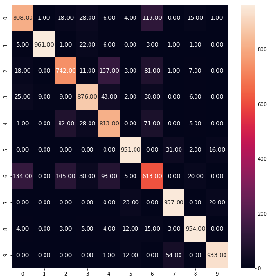 Figure 1
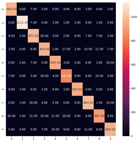 Figure 2
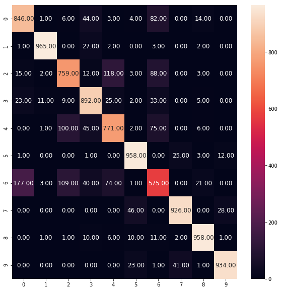 Figure 3
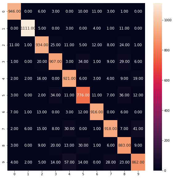 Figure 4
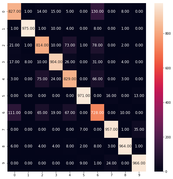 Figure 5
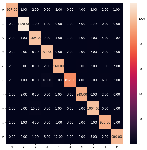 Figure 6
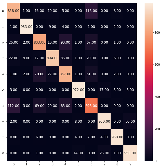 Figure 7
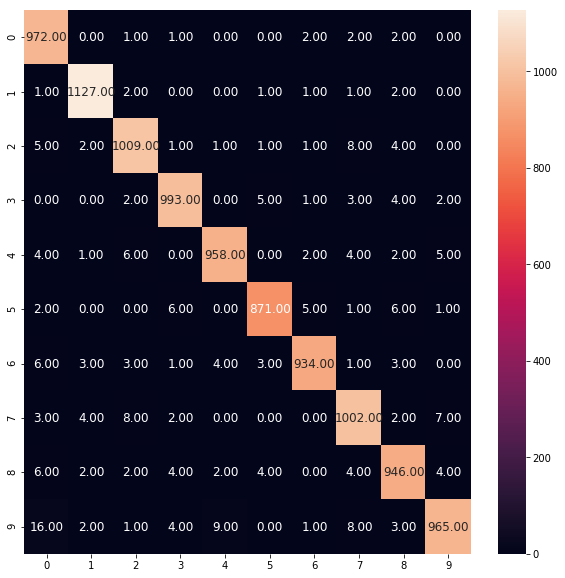 Figure 8
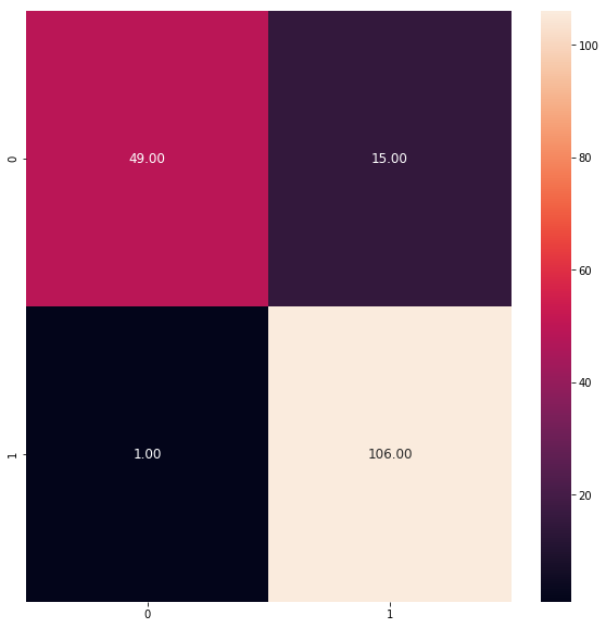 Figure 9
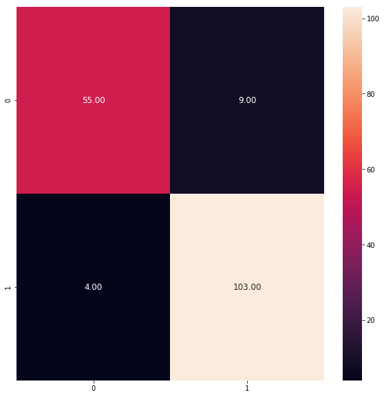 Figure 10
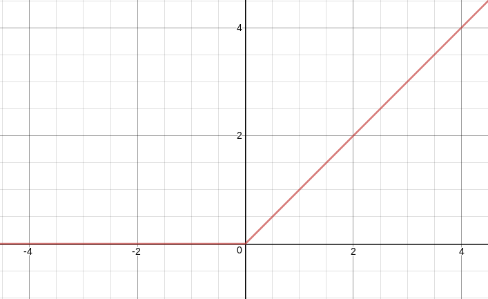 Figure 11
| Layer (type) | Output Shape | Param # |
|---|---|---|
| conv2d_1 (Conv2D) | (None, 14, 14, 32) | 320 |
| conv2d_2 (Conv2D) | (None, 12, 12, 32) | 9248 |
| max_pooling2d_1 (MaxPooling2) | (None, 6, 6, 32) | 0 |
| dropout_1 (Dropout) | (None, 6, 6, 32) | 0 |
| conv2d_3 (Conv2D) | (None, 4, 4, 64) | 18496 |
| conv2d_4 (Conv2D) | (None, 2, 2, 64) | 36928 |
| max_pooling2d_2 (MaxPooling2) | (None, 1, 1, 64) | 0 |
| dropout_2 (Dropout) | (None, 1, 1, 64) | 0 |
| flatten_1 (Flatten) | (None, 64) | 0 |
| dense_1 (Dense) | (None, 256) | 16640 |
| dropout_3 (Dropout) | (None, 256) | 0 |
| dense_2 (Dense) | (None, 10) | 2570 |
| Layer (type) | Output Shape | Param # |
|---|---|---|
| dense_3 (Dense) | (None, 512) | 131584 |
| dropout_4 (Dropout) | (None, 512) | 0 |
| dense_4 (Dense) | (None, 512) | 262656 |
| dropout_5 (Dropout) | (None, 512) | 0 |
| dense_5 (Dense) | (None, 512) | 262656 |
| dropout_6 (Dropout) | (None, 512) | 0 |
| dense_6 (Dense) | (None, 10) | 5130 |
| Metrics / Models | FFNN-Softmax | FFNN-ReLU |
|---|---|---|
| Training cross validation | ||
| Test accuracy | ||
| Precision | 0.98 | 0.98 |
| Recall | 0.98 | 0.98 |
| F1-score | 0.98 | 0.98 |
| Metrics / Models | CNN-Softmax | CNN-ReLU |
|---|---|---|
| Training cross validation | ||
| Test accuracy | ||
| Precision | 0.95 | 0.92 |
| Recall | 0.95 | 0.92 |
| F1-score | 0.95 | 0.92 |
| Fold # | Loss | Accuracy () |
|---|---|---|
| 1 | 1.9060128301398311 | 0.32963837901722315 |
| 2 | 1.4318902588488513 | 0.5091768125718277 |
| 3 | 1.362783239967884 | 0.5942213337366827 |
| 4 | 0.8257899198037331 | 0.7495911319797827 |
| 5 | 1.222473526516734 | 0.7038720233118376 |
| 6 | 0.4512576775334098 | 0.8729090907790444 |
| 7 | 0.49083630082824015 | 0.8601818182685158 |
| 8 | 0.34528968995411613 | 0.9032199380288064 |
| 9 | 0.30161443973038743 | 0.912663755545276 |
| 10 | 0.279967466075669 | 0.9171823807790317 |
| Metrics / Models | FFNN-Softmax | FFNN-ReLU |
|---|---|---|
| Training cross validation | ||
| Test accuracy | ||
| Precision | 0.89 | 0.89 |
| Recall | 0.89 | 0.89 |
| F1-score | 0.89 | 0.89 |
| Metrics / Models | CNN-Softmax | CNN-ReLU |
|---|---|---|
| Training cross validation | ||
| Test accuracy | ||
| Precision | 0.86 | 0.86 |
| Recall | 0.86 | 0.86 |
| F1-score | 0.86 | 0.86 |
| Fold # | Loss | Accuracy () |
|---|---|---|
| 1 | 0.7505188028133193 | 0.7309229651162791 |
| 2 | 0.6294445606858231 | 0.7821584302325582 |
| 3 | 0.5530192871624917 | 0.8128293656488342 |
| 4 | 0.468552251288519 | 0.8391494002614356 |
| 5 | 0.4499297190579501 | 0.8409090909090909 |
| 6 | 0.45004472223195163 | 0.8499999999566512 |
| 7 | 0.4096944159454683 | 0.855610110994295 |
| 8 | 0.39893951664539995 | 0.8681098779960613 |
| 9 | 0.37760543597664203 | 0.8637190683266308 |
| 10 | 0.34610279169377683 | 0.8804367606156083 |
| Metrics / Models | FFNN-Softmax | FFNN-ReLU |
|---|---|---|
| Training cross validation | ||
| Test accuracy | ||
| Precision | 0.92 | 0.91 |
| Recall | 0.92 | 0.91 |
| F1-score | 0.92 | 0.90 |
Peer Reviews
No public reviews on file for this paper yet. If you reviewed it on a platform where reviews are public (OpenReview, ICLR, NeurIPS, ICML), you can paste yours below so the community can read it here.
Code & Models
Videos
No videos yet. Explain this paper in a talk, walkthrough, or lecture? Add one.
Deep Learning using Rectified Linear Units (ReLU)
Abien Fred M. Agarap
(2017)
Abstract.
We introduce the use of rectified linear units (ReLU) as the classification function in a deep neural network (DNN). Conventionally, ReLU is used as an activation function in DNNs, with Softmax function as their classification function. However, there have been several studies on using a classification function other than Softmax, and this study is an addition to those. We accomplish this by taking the activation of the penultimate layer in a neural network, then multiply it by weight parameters to get the raw scores . Afterwards, we threshold the raw scores by [math], i.e. , where is the ReLU function. We provide class predictions through function, i.e. .
artificial intelligence; artificial neural networks; classification; convolutional neural network; deep learning; deep neural networks; feed-forward neural network; machine learning; rectified linear units; softmax; supervised learning
††copyright: none††conference: ; ; ††journalyear: 2017††ccs: Computing methodologies Supervised learning by classification††ccs: Computing methodologies Neural networks
1. Introduction
A number of studies that use deep learning approaches have claimed state-of-the-art performances in a considerable number of tasks such as image classification(Krizhevsky et al., 2012), natural language processing(Wen et al., 2015), speech recognition(Chorowski et al., 2015), and text classification(Yang et al., 2016). These deep learning models employ the conventional softmax function as the classification layer.
However, there have been several studies(Agarap, 2017; Alalshekmubarak and Smith, 2013; Tang, 2013) on using a classification function other than Softmax, and this study is yet another addition to those.
In this paper, we introduce the use of rectified linear units (ReLU) at the classification layer of a deep learning model. This approach is the novelty presented in this study, i.e. ReLU is conventionally used as an activation function for the hidden layers in a deep neural network. We accomplish this by taking the activation of the penultimate layer in a neural network, then use it to learn the weight parameters of the ReLU classification layer through backpropagation.
We demonstrate and compare the predictive performance of DL-ReLU models with DL-Softmax models on MNIST(LeCun et al., 2010), Fashion-MNIST(Xiao et al., 2017), and Wisconsin Diagnostic Breast Cancer (WDBC)(Wolberg et al., 1992) classification. We use the Adam(Kingma and Ba, 2014) optimization algorithm for learning the network weight parameters.
2. Methodology
2.1. Machine Intelligence Library
Keras(Chollet et al., 2015) with Google TensorFlow(Abadi et al., 2015) backend was used to implement the deep learning algorithms in this study, with the aid of other scientific computing libraries: matplotlib(Hunter, 2007), numpy(Walt et al., 2011), and scikit-learn(Pedregosa et al., 2011).
2.2. The Datasets
In this section, we describe the datasets used for the deep learning models used in the experiments.
2.2.1. MNIST
MNIST(LeCun et al., 2010) is one of the established standard datasets for benchmarking deep learning models. It is a 10-class classification problem having 60,000 training examples, and 10,000 test cases – all in grayscale, with each image having a resolution of .
2.2.2. Fashion-MNIST
Xiao et al. (2017)(Xiao et al., 2017) presented the new Fashion-MNIST dataset as an alternative to the conventional MNIST. The new dataset consists of grayscale images of fashion products from 10 classes, with images per class.
2.2.3. Wisconsin Diagnostic Breast Cancer (WDBC)
The WDBC dataset(Wolberg et al., 1992) consists of features which were computed from a digitized image of a fine needle aspirate (FNA) of a breast mass. There are 569 data points in this dataset: (1) 212 – Malignant, and (2) 357 – Benign.
2.3. Data Preprocessing
We normalized the dataset features using Eq. 1,
[TABLE]
where represents the dataset features, represents the mean value for each dataset feature , and represents the corresponding standard deviation. This normalization technique was implemented using the StandardScaler(Pedregosa et al., 2011) of scikit-learn.
For the case of MNIST and Fashion-MNIST, we employed Principal Component Analysis (PCA) for dimensionality reduction. That is, to select the representative features of image data. We accomplished this by using the PCA(Pedregosa et al., 2011) of scikit-learn.
2.4. The Model
We implemented a feed-forward neural network (FFNN) and a convolutional neural network (CNN), both of which had two different classification functions, i.e. (1) softmax, and (2) ReLU.
2.4.1. Softmax
Deep learning solutions to classification problems usually employ the softmax function as their classification function (last layer). The softmax function specifies a discrete probability distribution for classes, denoted by .
If we take as the activation at the penultimate layer of a neural network, and as its weight parameters at the softmax layer, we have as the input to the softmax layer,
[TABLE]
Consequently, we have
[TABLE]
Hence, the predicted class would be
[TABLE]
2.4.2. Rectified Linear Units (ReLU)
ReLU is an activation function introduced by (Hahnloser et al., 2000), which has strong biological and mathematical underpinning. In 2011, it was demonstrated to further improve training of deep neural networks. It works by thresholding values at 0, i.e. . Simply put, it outputs 0 when , and conversely, it outputs a linear function when (refer to Figure 1 for visual representation).
We propose to use ReLU not only as an activation function in each hidden layer of a neural network, but also as the classification function at the last layer of a network.
Hence, the predicted class for ReLU classifier would be ,
[TABLE]
2.4.3. Deep Learning using ReLU
ReLU is conventionally used as an activation function for neural networks, with softmax being their classification function. Then, such networks use the softmax cross-entropy function to learn the weight parameters of the neural network. In this paper, we still implemented the mentioned loss function, but with the distinction of using the ReLU for the prediction units (see Eq. 6). The parameters are then learned by backpropagating the gradients from the ReLU classifier. To accomplish this, we differentiate the ReLU-based cross-entropy function (see Eq. 7) w.r.t. the activation of the penultimate layer,
[TABLE]
Let the input be replaced the penultimate activation output ,
[TABLE]
The backpropagation algorithm (see Eq. 8) is the same as the conventional softmax-based deep neural network.
[TABLE]
Algorithm 1 shows the rudimentary gradient-descent algorithm for a DL-ReLU model.
In some experiments, we found the DL-ReLU models perform on par with the softmax-based models.
2.5. Data Analysis
To evaluate the performance of the DL-ReLU models, we employ the following metrics:
- (1)
Cross Validation Accuracy & Standard Deviation. The result of -fold CV experiments. 2. (2)
Test Accuracy. The trained model performance on unseen data. 3. (3)
Recall, Precision, and F1-score. The classification statistics on class predictions. 4. (4)
Confusion Matrix. The table for describing classification performance.
3. Experiments
All experiments in this study were conducted on a laptop computer with Intel Core(TM) i5-6300HQ CPU @ 2.30GHz x 4, 16GB of DDR3 RAM, and NVIDIA GeForce GTX 960M 4GB DDR5 GPU.
Table 1 shows the architecture of the VGG-like CNN (from Keras(Chollet et al., 2015)) used in the experiments. The last layer, dense_2, used the softmax classifier and ReLU classifier in the experiments.
The Softmax- and ReLU-based models had the same hyper-parameters, and it may be seen on the Jupyter Notebook found in the project repository: https://github.com/AFAgarap/relu-classifier.
Table 2 shows the architecture of the feed-forward neural network used in the experiments. The last layer, dense_6, used the softmax classifier and ReLU classifier in the experiments.
All models used Adam(Kingma and Ba, 2014) optimization algorithm for training, with the default learning rate , , , , and no decay.
3.1. MNIST
We implemented both CNN and FFNN defined in Tables 1 and 2 on a normalized, and PCA-reduced features, i.e. from (784) dimensions down to (256) dimensions.
In training a FFNN with two hidden layers for MNIST classification, we found the results described in Table 3.
Despite the fact that the Softmax-based FFNN had a slightly higher test accuracy than the ReLU-based FFNN, both models had 0.98 for their F1-score. These results imply that the FFNN-ReLU is on par with the conventional FFNN-Softmax.
Figures 2 and 3 show the predictive performance of both models for MNIST classification on its 10 classes. Values of correct prediction in the matrices seem to be balanced, as in some classes, the ReLU-based FFNN outperformed the Softmax-based FFNN, and vice-versa.
In training a VGG-like CNN(Chollet et al., 2015) for MNIST classification, we found the results described in Table 4.
The CNN-ReLU was outperformed by the CNN-Softmax since it converged slower, as the training accuracies in cross validation were inspected (see Table 5). However, despite its slower convergence, it was able to achieve a test accuracy higher than 90%. Granted, it is lower than the test accuracy of CNN-Softmax by , but further optimization may be done on the CNN-ReLU to achieve an on-par performance with the CNN-Softmax.
Figures 4 and 5 show the predictive performance of both models for MNIST classification on its 10 classes. Since the CNN-Softmax converged faster than CNN-ReLU, it has the most number of correct predictions per class.
3.2. Fashion-MNIST
We implemented both CNN and FFNN defined in Tables 1 and 2 on a normalized, and PCA-reduced features, i.e. from (784) dimensions down to (256) dimensions. The dimensionality reduction for MNIST was the same for Fashion-MNIST for fair comparison. Though this discretion may be challenged for further investigation.
In training a FFNN with two hidden layers for Fashion-MNIST classification, we found the results described in Table 6.
Despite the fact that the Softmax-based FFNN had a slightly higher test accuracy than the ReLU-based FFNN, both models had 0.89 for their F1-score. These results imply that the FFNN-ReLU is on par with the conventional FFNN-Softmax.
Figures 6 and 7 show the predictive performance of both models for Fashion-MNIST classification on its 10 classes. Values of correct prediction in the matrices seem to be balanced, as in some classes, the ReLU-based FFNN outperformed the Softmax-based FFNN, and vice-versa.
In training a VGG-like CNN(Chollet et al., 2015) for Fashion-MNIST classification, we found the results described in Table 7.
Similar to the findings in MNIST classification, the CNN-ReLU was outperformed by the CNN-Softmax since it converged slower, as the training accuracies in cross validation were inspected (see Table 8). Despite its slightly lower test accuracy, the CNN-ReLU had the same F1-score of 0.86 with CNN-Softmax – also similar to the findings in MNIST classification.
Figures 8 and 9 show the predictive performance of both models for Fashion-MNIST classification on its 10 classes. Contrary to the findings of MNIST classification, CNN-ReLU had the most number of correct predictions per class. Conversely, with its faster convergence, CNN-Softmax had the higher cumulative correct predictions per class.
3.3. WDBC
We implemented FFNN defined in Table 2, but with hidden layers having 64 neurons followed by 32 neurons instead of two hidden layers both having 512 neurons. For the WDBC classfication, we only normalized the dataset features. PCA dimensionality reduction might not prove to be prolific since WDBC has only 30 features.
In training the FFNN with two hidden layers of neurons, we found the results described in Table 9.
Similar to the findings in classification using CNN-based models, the FFNN-ReLU was outperformed by the FFNN-Softmax in WDBC classification. Consistent with the CNN-based models, the FFNN-ReLU suffered from slower convergence than the FFNN-Softmax. However, there was only 0.2 F1-score difference between them. It stands to reason that the FFNN-ReLU is still comparable with FFNN-Softmax.
Figures 10 and 11 show the predictive performance of both models for WDBC classification on binary classification. The confusion matrices show that the FFNN-Softmax had more false negatives than FFNN-ReLU. Conversely, FFNN-ReLU had more false positives than FFNN-Softmax.
4. Conclusion and Recommendation
The relatively unfavorable findings on DL-ReLU models is most probably due to the dying neurons problem in ReLU. That is, no gradients flow backward through the neurons, and so, the neurons become stuck, then eventually “die”. In effect, this impedes the learning progress of a neural network. This problem is addressed in subsequent improvements on ReLU (e.g. (Trottier et al., 2017)). Aside from such drawback, it may be stated that DL-ReLU models are still comparable to, if not better than, the conventional Softmax-based DL models. This is supported by the findings in DNN-ReLU for image classification using MNIST and Fashion-MNIST.
Future work may be done on thorough investigation of DL-ReLU models through numerical inspection of gradients during backpropagation, i.e. compare the gradients in DL-ReLU models with the gradients in DL-Softmax models. Furthermore, ReLU variants may be brought into the table for additional comparison.
5. Acknowledgment
An appreciation of the VGG-like Convnet source code in Keras(Chollet et al., 2015), as it was the CNN model used in this study.
The reference list from the paper itself. Each links out to its DOI / PubMed record.
- 1(1)
- 2Abadi et al . (2015) Martín Abadi, Ashish Agarwal, Paul Barham, Eugene Brevdo, Zhifeng Chen, Craig Citro, Greg S. Corrado, Andy Davis, Jeffrey Dean, Matthieu Devin, Sanjay Ghemawat, Ian Goodfellow, Andrew Harp, Geoffrey Irving, Michael Isard, Yangqing Jia, Rafal Jozefowicz, Lukasz Kaiser, Manjunath Kudlur, Josh Levenberg, Dan Mané, Rajat Monga, Sherry Moore, Derek Murray, Chris Olah, Mike Schuster, Jonathon Shlens, Benoit Steiner, Ilya Sutskever, Kunal Talwar, Paul Tucker, Vincent Vanhoucke,
- 3Agarap (2017) Abien Fred Agarap. 2017. A Neural Network Architecture Combining Gated Recurrent Unit (GRU) and Support Vector Machine (SVM) for Intrusion Detection in Network Traffic Data. ar Xiv preprint ar Xiv:1709.03082 (2017).
- 4Alalshekmubarak and Smith (2013) Abdulrahman Alalshekmubarak and Leslie S Smith. 2013. A novel approach combining recurrent neural network and support vector machines for time series classification. In Innovations in Information Technology (IIT), 2013 9th International Conference on . IEEE, 42–47.
- 5Chollet et al . (2015) François Chollet et al . 2015. Keras. https://github.com/keras-team/keras . (2015).
- 6Chorowski et al . (2015) Jan K Chorowski, Dzmitry Bahdanau, Dmitriy Serdyuk, Kyunghyun Cho, and Yoshua Bengio. 2015. Attention-based models for speech recognition. In Advances in Neural Information Processing Systems . 577–585.
- 7Hahnloser et al . (2000) Richard HR Hahnloser, Rahul Sarpeshkar, Misha A Mahowald, Rodney J Douglas, and H Sebastian Seung. 2000. Digital selection and analogue amplification coexist in a cortex-inspired silicon circuit. Nature 405, 6789 (2000), 947.
- 8Hunter (2007) J. D. Hunter. 2007. Matplotlib: A 2D graphics environment. Computing In Science & Engineering 9, 3 (2007), 90–95. https://doi.org/10.1109/MCSE.2007.55 · doi ↗
