TL;DR
This paper introduces an efficient Bayesian method for inferring large Gaussian graphical models by using closed-form Bayes factors for hypothesis testing, enabling scalable analysis of high-dimensional data.
Contribution
It develops a computationally efficient approach with exact tail probabilities for Bayesian inference in large Gaussian graphical models, addressing high-dimensional challenges.
Findings
Method performs well on simulated data
Successfully applied to large gene expression dataset
Controls error rates effectively in edge selection
Abstract
Despite major methodological developments, Bayesian inference for Gaussian graphical models remains challenging in high dimension due to the tremendous size of the model space. This article proposes a method to infer the marginal and conditional independence structures between variables by multiple testing of hypotheses. Specifically, we introduce closed-form Bayes factors under the Gaussian conjugate model to evaluate the null hypotheses of marginal and conditional independence between variables. Their computation for all pairs of variables is shown to be extremely efficient, thereby allowing us to address large problems with thousands of nodes. Moreover, we derive exact tail probabilities from the null distributions of the Bayes factors. These allow the use of any multiplicity correction procedure to control error rates for incorrect edge inclusion. We demonstrate the proposed…
Click any figure to enlarge with its caption.
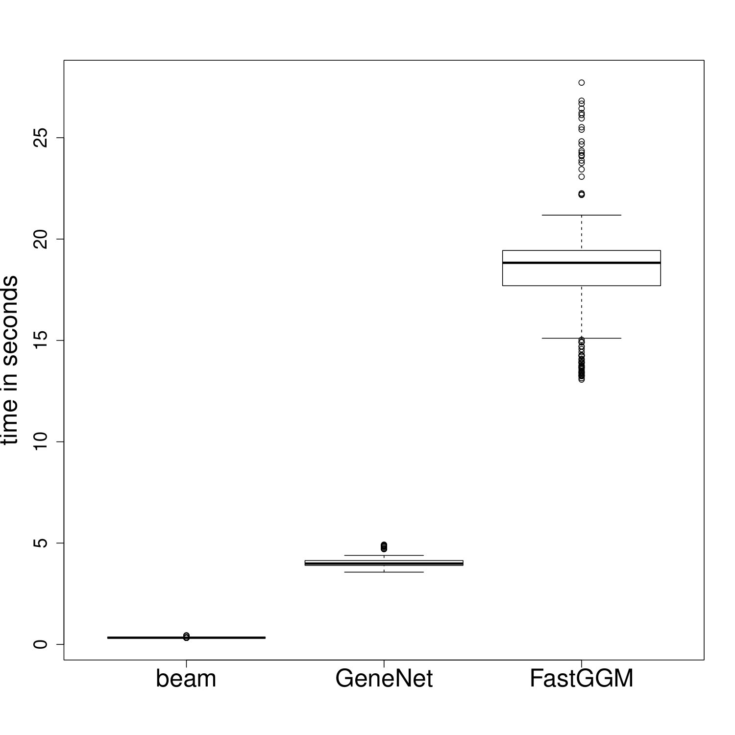 Figure 1
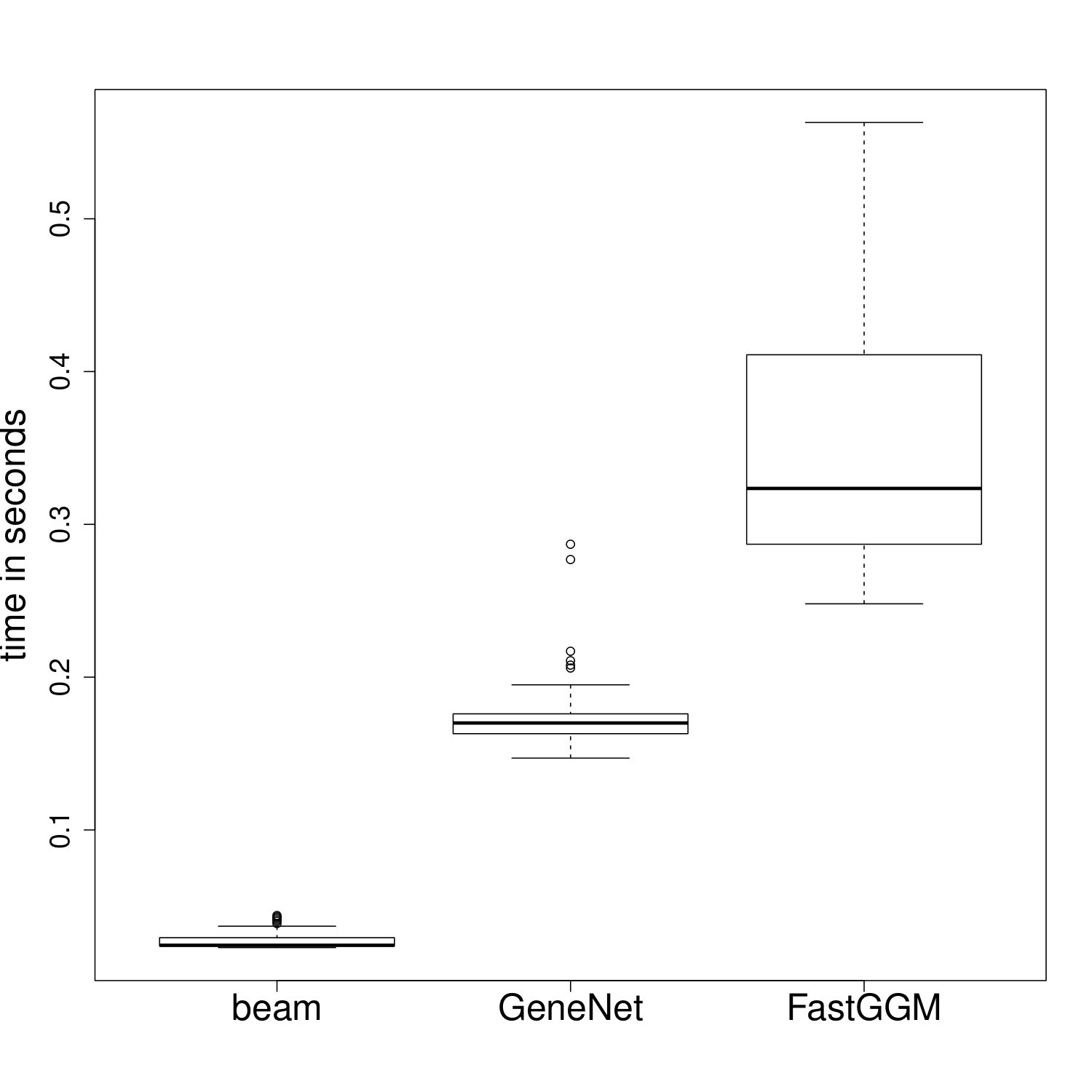 Figure 2
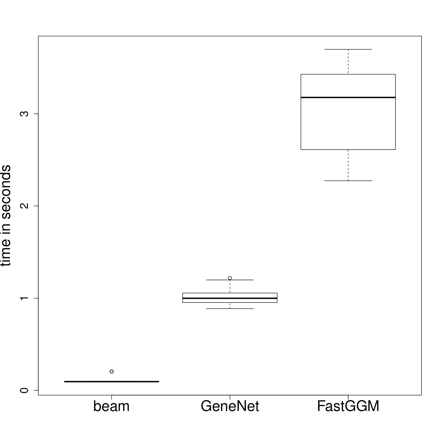 Figure 3
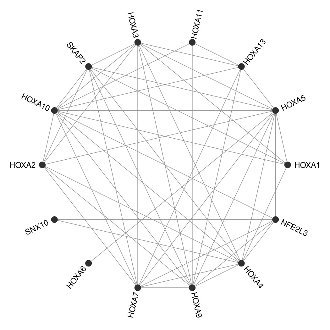 Figure 4
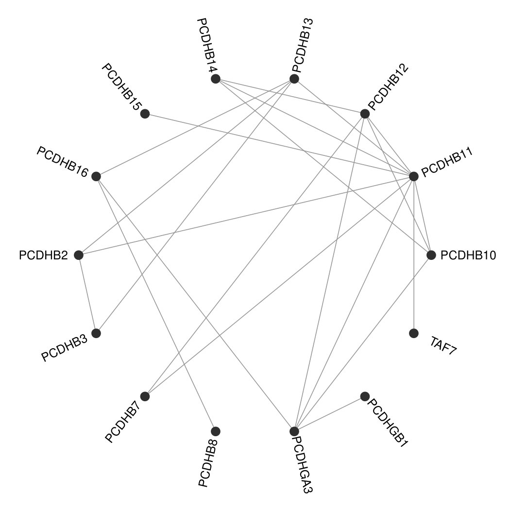 Figure 5
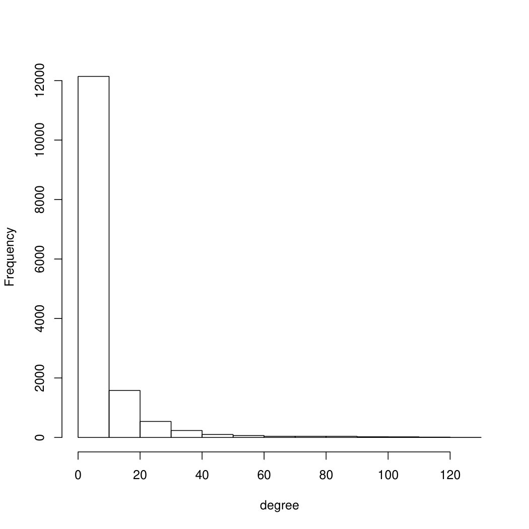 Figure 6
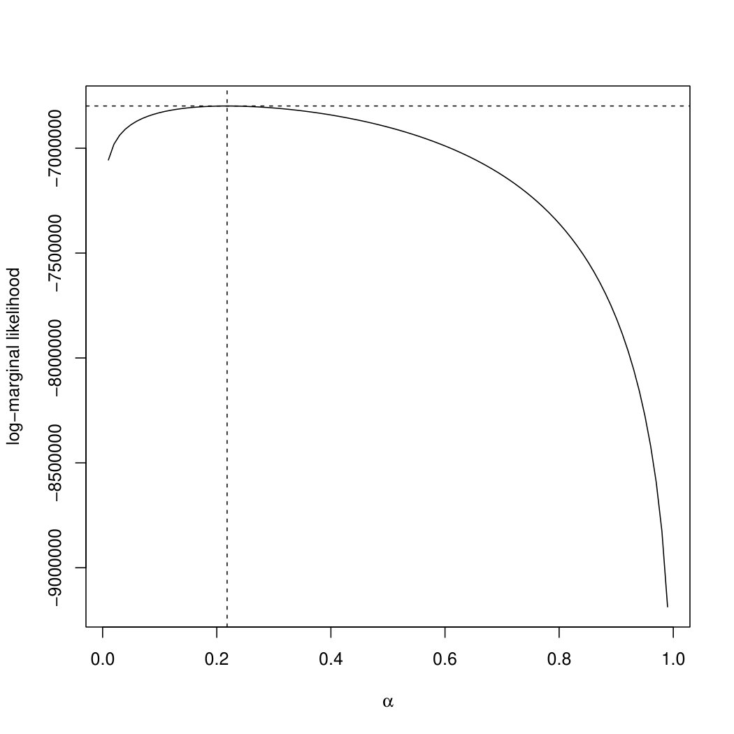 Figure 7
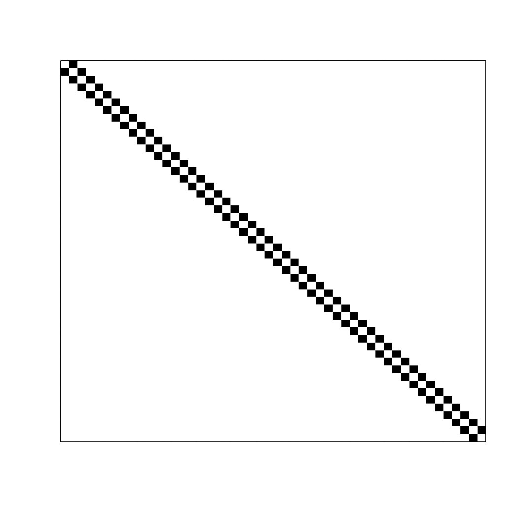 Figure 8
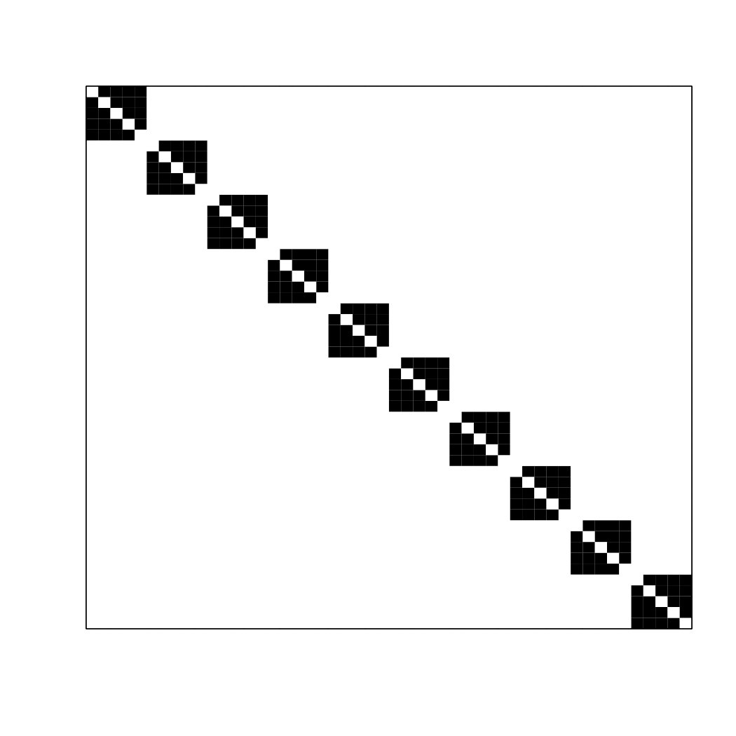 Figure 9
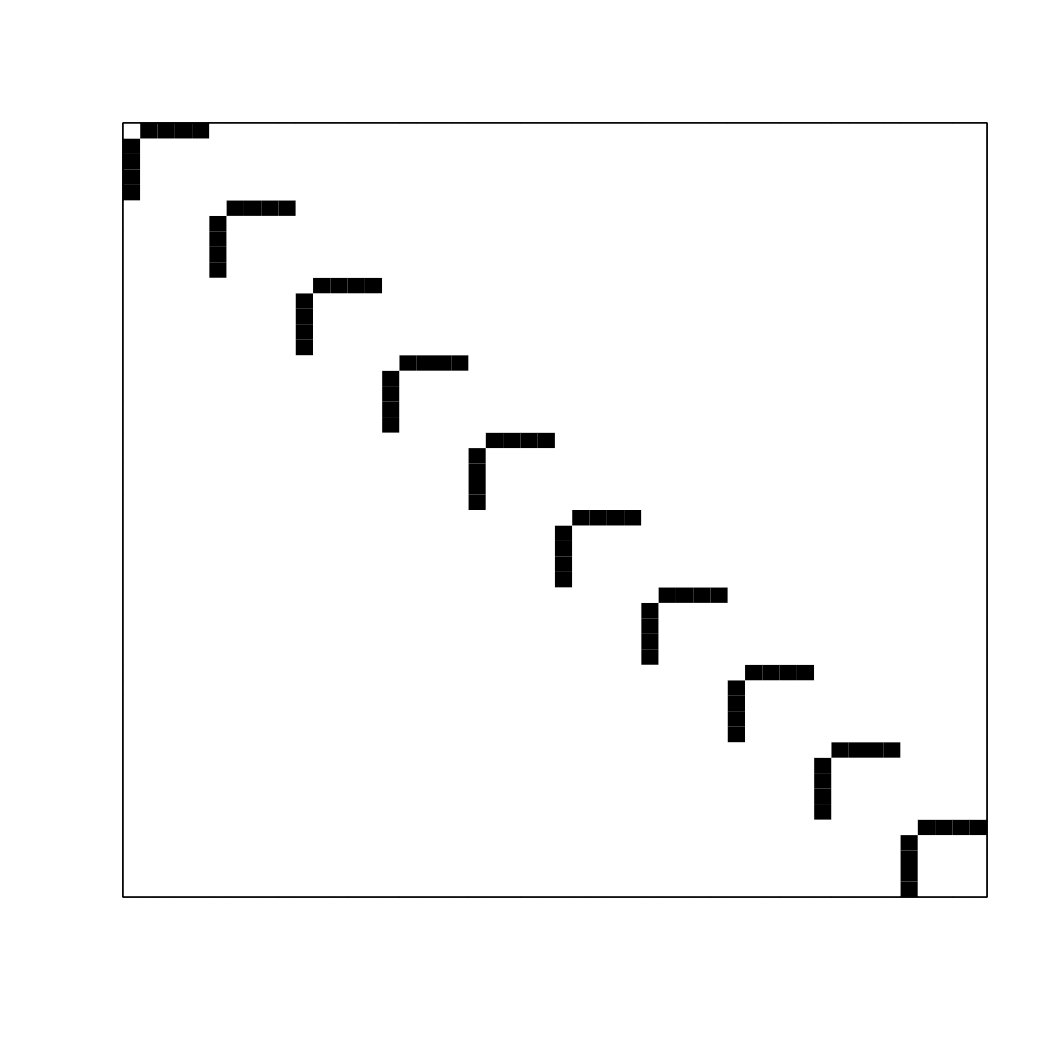 Figure 10
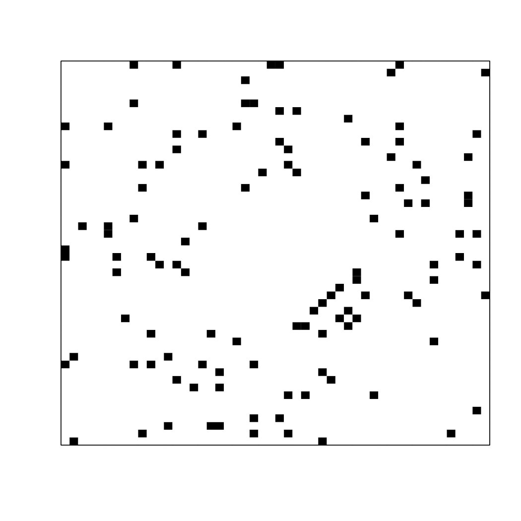 Figure 11
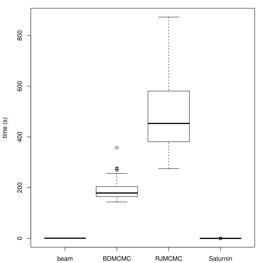 Figure 12
| Method | AUC | AUC | AUC | AUC | |
|---|---|---|---|---|---|
| Band structure | Cluster structure | ||||
| 100 | beam | 0.89 (0.02) | 0.65 (0.03) | 0.80 (0.02) | 0.54 (0.03) |
| 100 | bdmcmc | 0.89 (0.03) | 0.67 (0.03) | 0.79 (0.02) | 0.51 (0.04) |
| 100 | rjmcmc | 0.88 (0.03) | 0.63 (0.05) | 0.78 (0.03) | 0.50 (0.04) |
| 100 | saturnin | 0.89 (0.02) | 0.61 (0.04) | 0.77 (0.02) | 0.53 (0.04) |
| 50 | beam | 0.84 (0.03) | 0.53 (0.04) | 0.73 (0.02) | 0.39 (0.04) |
| 50 | bdmcmc | 0.82 (0.03) | 0.51 (0.06) | 0.72 (0.03) | 0.37 (0.04) |
| 50 | rjmcmc | 0.81 (0.03) | 0.47 (0.05) | 0.72 (0.02) | 0.35 (0.04) |
| 50 | saturnin | 0.82 (0.02) | 0.44 (0.04) | 0.68 (0.02) | 0.33 (0.04) |
| 25 | beam | 0.78 (0.04) | 0.39 (0.05) | 0.66 (0.03) | 0.24 (0.04) |
| 25 | bdmcmc | 0.75 (0.04) | 0.32 (0.05) | 0.65 (0.03) | 0.23 (0.03) |
| 25 | rjmcmc | 0.75 (0.04) | 0.27 (0.05) | 0.64 (0.03) | 0.22 (0.03) |
| 25 | saturnin | 0.73 (0.03) | 0.28 (0.05) | 0.58 (0.02) | 0.15 (0.02) |
| Hub structure | Random structure | ||||
| 100 | beam | 0.88 (0.03) | 0.62 (0.03) | 0.87 (0.03) | 0.65 (0.03) |
| 100 | bdmcmc | 0.89 (0.02) | 0.67 (0.04) | 0.86 (0.03) | 0.66 (0.03) |
| 100 | rjmcmc | 0.89 (0.02) | 0.65 (0.05) | 0.85 (0.03) | 0.65 (0.04) |
| 100 | saturnin | 0.92 (0.01) | 0.63 (0.02) | 0.86 (0.02) | 0.59 (0.02) |
| 50 | beam | 0.84 (0.03) | 0.53 (0.03) | 0.83 (0.03) | 0.56 (0.04) |
| 50 | bdmcmc | 0.84 (0.03) | 0.52 (0.05) | 0.81 (0.03) | 0.53 (0.05) |
| 50 | rjmcmc | 0.84 (0.03) | 0.48 (0.06) | 0.80 (0.03) | 0.49 (0.06) |
| 50 | saturnin | 0.86 (0.02) | 0.48 (0.03) | 0.83 (0.02) | 0.47 (0.03) |
| 25 | beam | 0.80 (0.03) | 0.42 (0.04) | 0.79 (0.03) | 0.43 (0.05) |
| 25 | bdmcmc | 0.79 (0.04) | 0.32 (0.05) | 0.75 (0.02) | 0.33 (0.05) |
| 25 | rjmcmc | 0.77 (0.04) | 0.27 (0.04) | 0.74 (0.03) | 0.30 (0.05) |
| 25 | saturnin | 0.80 (0.03) | 0.35 (0.04) | 0.77 (0.02) | 0.35 (0.04) |
| Method | AUC | AUC | AUC | AUC | |
|---|---|---|---|---|---|
| Band structure | Cluster structure | ||||
| 200 | beam | 0.88 (0.01) | 0.55 (0.02) | 0.91 (0.01) | 0.58 (0.01) |
| 200 | GeneNet | 0.89 (0.01) | 0.57 (0.02) | 0.91 (0.01) | 0.59 (0.01) |
| 200 | FastGGM | 0.87 (0.01) | 0.57 (0.02) | 0.89 (0.01) | 0.60 (0.02) |
| 500 | beam | 0.91 (0.01) | 0.58 (0.01) | 0.89 (0.01) | 0.50 (0.01) |
| 500 | GeneNet | 0.91 (0.01) | 0.60 (0.01) | 0.89 (0.01) | 0.52 (0.01) |
| 500 | FastGGM | 0.90 (0.01) | 0.61 (0.01) | 0.85 (0.01) | 0.49 (0.01) |
| 1000 | beam | 0.88 (0.01) | 0.49 (0.01) | 0.90 (0.00) | 0.48 (0.01) |
| 1000 | GeneNet | 0.88 (0.01) | 0.49 (0.01) | 0.90 (0.00) | 0.49 (0.01) |
| 1000 | FastGGM | 0.87 (0.01) | 0.51 (0.01) | 0.87 (0.00) | 0.48 (0.01) |
| Hub structure | Random structure | ||||
| 200 | beam | 0.90 (0.01) | 0.56 (0.01) | 0.86 (0.01) | 0.43 (0.02) |
| 200 | GeneNet | 0.85 (0.01) | 0.21 (0.03) | 0.86 (0.01) | 0.47 (0.02) |
| 200 | FastGGM | 0.87 (0.01) | 0.46 (0.02) | 0.85 (0.01) | 0.47 (0.02) |
| 500 | beam | 0.92 (0.01) | 0.54 (0.01) | 0.82 (0.01) | 0.35 (0.01) |
| 500 | GeneNet | 0.90 (0.00) | 0.43 (0.01) | 0.82 (0.01) | 0.34 (0.01) |
| 500 | FastGGM | 0.88 (0.01) | 0.44 (0.01) | 0.81 (0.00) | 0.34 (0.01) |
| 1000 | beam | 0.93 (0.00) | 0.54 (0.01) | 0.77 (0.00) | 0.22 (0.01) |
| 1000 | GeneNet | 0.92 (0.00) | 0.49 (0.01) | 0.77 (0.00) | 0.21 (0.01) |
| 1000 | FastGGM | 0.89 (0.00) | 0.44 (0.01) | 0.77 (0.00) | 0.22 (0.01) |
Peer Reviews
No public reviews on file for this paper yet. If you reviewed it on a platform where reviews are public (OpenReview, ICLR, NeurIPS, ICML), you can paste yours below so the community can read it here.
Code & Models
Videos
No videos yet. Explain this paper in a talk, walkthrough, or lecture? Add one.
**Fast Bayesian inference in large Gaussian graphical models
**
Gwenaël G.R. Leday and Sylvia Richardson
MRC Biostatistics Unit, University of Cambridge, UK
Abstract
Despite major methodological developments, Bayesian inference for Gaussian graphical models remains challenging in high dimension due to the tremendous size of the model space. This article proposes a method to infer the marginal and conditional independence structures between variables by multiple testing of hypotheses. Specifically, we introduce closed-form Bayes factors under the Gaussian conjugate model to evaluate the null hypotheses of marginal and conditional independence between variables. Their computation for all pairs of variables is shown to be extremely efficient, thereby allowing us to address large problems with thousands of nodes. Moreover, we derive exact tail probabilities from the null distributions of the Bayes factors. These allow the use of any multiplicity correction procedure to control error rates for incorrect edge inclusion. We demonstrate the proposed approach to graphical model selection on various simulated examples as well as on a large gene expression data set from The Cancer Genome Atlas.
1 Introduction
Graphical models provide a natural basis for the statistical description and analysis of interplay between variables. In applications, interest often lies in the bidirected and undirected graphs that respectively describe the marginal and conditional dependence structures among variables (Wang,, 2015). When the joint distribution of the variables is assumed to be Gaussian, these are known to be fully coded in the covariance matrix and its inverse (Dempster,, 1972, Cox and Wermuth,, 1993). Precisely, a pair of variables with , will be marginally independent when and conditionally independent (given all the remaining variables) when . The present article treats inference of both types of graphs in context of the Gaussian model when the number of variables is large.
Despite major methodological developments, Bayesian inference for Gaussian graphical models remains challenging. The standard approach casts the problem as a model selection problem, and first requires specification of prior distributions over all possible graphical models and their parameter spaces. Such specification is not straightforward as it is desirable to favour parsimonious models and address the compatibility of priors across models (Carvalho and Scott,, 2009, Consonni and La Rocca,, 2012). Next, the inference procedure is hindered by the search over a very high-dimensional model space where the number of possible graphical models grows super-exponentially with the number of variables. Full exploration of the model space is, therefore, only possible when the number of variables is very small (say ). In moderate- and high-dimensional settings where is in the tens, hundreds or thousands, the model space must generally be searched stochastically (Mohammadi and Wit,, 2015, Wang and Li,, 2012, Lenkoski and Dobra,, 2011, Giudici and Green,, 1999). However, due to the tremendous size of the model space in such settings, it may be difficult (nay impossible) to identify with confidence the graphical model that is best supported by the data. Accordingly, it has become common practice to account for model uncertainty by performing Bayesian model averaging and infer the graphical structure by selecting edges with the highest marginal posterior probabilities, for example by exploiting their connection to a Bayesian version of the false discovery rate (Mitra et al.,, 2013, Peterson et al.,, 2015, Baladandayuthapani et al.,, 2014).
To tackle the difficulties associated with the standard approach this article proposes a method to directly select edges by multiple testing of hypotheses about pairwise (marginal or conditional) independence (Drton and Perlman,, 2007) using closed-form Bayes factors. These are obtained using the conditional approach of Dickey, (1971), in which the prior under the null hypothesis is derived from that of the alternative by conditioning on the null hypothesis. This approach was also adopted by Giudici, (1995) to derive a closed-form Bayes factor for conditional independence. However, the latter relies on elements of the inverse of the sample covariance matrix which is singular when the number of variables is large relative to the sample size. We bypass this issue and also introduce a closed-form Bayes factor for marginal independence. Moreover, we show the consistency of the Bayes factors and derive exact tail probabilities from their null distributions to help address the multiplicity problem and control error rates for incorrect edge inclusion. The proposed procedure, available via the R package beam on the CRAN website (R Core Team,, 2016, http://cran.r-project.org), is shown to be computationally very efficient, addressing problems with thousands of nodes in just a few seconds.
The article is structured as follows. The next section introduces basic notations and the Gaussian conjugate model. In section 3 we present closed-form Bayes factors to evaluate the null hypotheses of marginal and conditional independence between any two variables and study their consistency. Section 4 details graph inference and discuss the multiple testing problem and error control. The performance of the proposed approach is compared to Bayesian and non-Bayesian methods on simulated data in section 5. Section 6 illustrates our method on a large gene expression data set from The Cancer Genome Atlas.
2 Background
2.1 Notation
The following notation will be used throughout this paper. We employ the notation to say that the random column vector , has a multivariate normal distribution with mean and positive definite covariance matrix . We also write to indicate that the random matrix with density
[TABLE]
has a Wishart distribution with scale matrix and degrees of freedom . Here represents the determinant of , denotes the trace of matrix and is the multivariate gamma function. The inverse of is said to have an Inverse-Wishart distribution with scale matrix and degrees of freedom. We shall use the notation . A random variable following a beta distribution with shape parameters and will be denoted by . We use the operator to denote the linear transformation that stacks the columns of a matrix into a vector and to denote the Kronecker product. We refer to Gupta and Nagar, (2000) for more details on these operators. Last, we shall use the subscripts , , and to refer to the submatrices , , and of a symmetric matrix whose block-wise decomposition is implied by a partition of its rows and columns into two disjoint subsets indexed by and .
2.2 The Gaussian conjugate model
Given an observation matrix the Gaussian conjugate model is defined by
[TABLE]
with positive definite, the -dimensional identity matrix and . Here, the covariance matrix with kronecker product structure makes explicit the assumption of independence for the rows of and the dependence of its columns via the covariance .
Due to conjugacy, model (1) offers closed-form Bayesian estimators of the covariance matrix and its inverse . The posterior expectation of is
[TABLE]
where , and that of its inverse is
[TABLE]
It is important to note that estimator (2) is a linear shrinkage estimator that is a convex linear combination between the maximum likelihood estimator of and , with weight (Chen,, 1979, Hannart and Naveau,, 2014). Likewise, estimator (3) is recognized as a ridge-type estimator of the precision matrix (Kubokawa and Srivastava,, 2008, Van Wieringen and Peeters,, 2016). The next proposition presents some properties of these two estimators. All proofs are presented in the Appendix.
Proposition 1**.**
Let estimators (2) and (3) depend on with , and fixed, and denote them by and , respectively. Then the following properties hold:
- (i)
** 2. (ii)
** 3. (iii)
** 4. (iv)
, if , 5. (v)
* and are positive definite*
Additionally, the asymptotic properties of estimators (2) and (3) when are the same as those of the maximum likelihood estimators and of and . Proposition 2 summarizes.
Proposition 2**.**
Let estimator (2) and (3) depend on with , and be fixed, and denote them by and , respectively. Then the following properties hold:
- (i)
** 2. (ii)
**
2.3 Choice of hyperparameters
In model 1, the prior matrix represents the prior expectation of . It may also be interpreted as the shrinkage target towards which the maximum likelihood estimator of the covariance matrix is shrunk, since the posterior expectation of is a linear shrinkage estimator. For these reasons, can be chosen to encourage estimator (2) to have specific structures (e.g. autoregressives or low-ranks). Ideally, in such cases the matrix should be parameterised by a low-dimensional vector of hyperparameters that are interpretable and for which prior knowledge exists. As often this knowledge is absent, it is common to choose . Throughout this paper we use and standardize the observation matrix so that for , and , where is an vector whose elements are all equal to 1.
The other hyperparameter clearly acts as a regularization parameter (see equation (2) and (3)) and its value must therefore be chosen carefully. Following Chen, (1979) and Hannart and Naveau, (2014) we use empirical Bayes and estimate by the value maximizing the marginal (or integrated) likelihood of the model, i.e. by
[TABLE]
where
[TABLE]
The above optimization problem is easily solved because the marginal likelihood is concave in . Moreover, remark that and , where and are respectively the r and l largest eigenvalues of and . Hence, evaluating the objective function for different values of is computationally cheap provided the eigenvalues of and have been pre-computed. We are referring the reader to Hannart and Naveau, (2014, Section 2.3.) for the proof that the asymptotic properties of estimator (2) and (3) (Proposition 1) hold when .
3 Bayes factors
3.1 Bayes factor for conditional independence
In this section we derive an analytic expression for the Bayes factor evaluating the null hypothesis of conditional independence between two variables in context of model (1). For ease of notation we define and . We wish to evaluate the null hypothesis of conditional independence, denoted , between two coordinates and , . We test against the alternative hypothesis , where is the element of . The Bayes factor evaluating evidence in favour of is
[TABLE]
where, by definition, is such that .
Giudici, (1995) showed that (4) could be obtained in closed-form by reparameterising the Gaussian conjugate model and defining a compatible prior under the null hypothesis using the approach of Dickey, (1971). However, the proposed Bayes factor does not exist in high dimensional settings because it depends on elements of . This problem is here circumvented by factorising the joint likelihood of the observed data as
[TABLE]
the product of a marginal and conditional likelihood. This factorisation arises from the partition of into two disjoint subsets indexed by and . The quantity represents the matrix of regression coefficients obtained when regressing the variables indexed by onto the variables indexed by , whereas denotes the residual covariance matrix.
The factorisation of the likelihood allows conveniently to simplify (4). Using the change of variable from to together with the fact that is independent of , most nuisance parameters are integrated out and equation (4) becomes
[TABLE]
Note that by the standard properties of the multivariate normal and Inverse-Wishart distributions Gupta and Nagar, (2000, Theorems 2.3.12. and 3.3.9.) the densities under the alternative model are
[TABLE]
where and . Therefore, the simplification of Bayes factor (4) intuitively tells us that evaluating the conditional independence between any two coordinates within the -dimensional Gaussian conjugate model (1) is equivalent to evaluating the diagonality of the residual covariance matrix in a bivariate response regression model.
To obtain (5) in closed-form we, similarly to Giudici, (1995), define a compatible prior for under the null hypothesis using the conditional approach of Dickey, (1971). Precisely, the prior density under is derived from that under by conditioning on . The densities under the null model are therefore
[TABLE]
where is such that .
We now state the main result of this section.
Lemma 1**.**
Assume (5) holds with densities defined by (6) and (7). Then the Bayes factor in favour of is
[TABLE]
with F_{aa.b}=\left[\begin{array}[]{cc}g_{ii}&g_{ij}\\ g_{ij}&g_{jj}\end{array}\right], , T_{aa.b}=\left[\begin{array}[]{cc}q_{ii}&q_{ij}\\ q_{ij}&q_{jj}\end{array}\right] and .
Remark 1**.**
In Lemma 1, the quantities and (resp. and ) can be thought of representing prior and posterior partial variances for coordinate (resp. ), whereas and can be thought of representing prior and posterior partial correlations.
Remark 2**.**
The Bayes factor proposed by Giudici, (1995, lemma 3), in contrast to Lemma 1, defines the quantities and such that the matrices and , with . Note that here only exists when is invertible (i.e. when is large relatively to ) whereas defined in Lemma 1 exists even when because is always positive definite (a consequence of Proposition 1).
Remark 3**.**
Standard matrix algebra (Gupta and Nagar,, 2000, Theorem 1.2.3.v) tells us that and . This means that the elements of the matrices and can respectively be obtained from the elements of and . The computation of the Bayes factor in Lemma 1 for all pairs of variables , , hence boils down to computing and .
3.2 Bayes factor for marginal independence
We now derive an analytic expression for the Bayes factor evaluating the null hypothesis of marginal independence between any two variables in context of model (1). We test against the alternative hypothesis , where is the element of . The Bayes factor evaluating evidence in favour of is
[TABLE]
where now is such that .
We adopt a similar approach as in section 3.1 to obtain (8) in closed-form. We first write the joint likelihood as
[TABLE]
and make a change of variable from to , where and . Then, using the fact that is independent of it is easily seen that the Bayes factor (8) simplifies to
[TABLE]
Here, the densities under the alternative model, by properties of the multivariate normal and Inverse-Wishart distributions, are
[TABLE]
whereas the densities under the null model are
[TABLE]
We now state the following lemma.
Lemma 2**.**
Assume (9) holds with densities defined by (10) and (11). Then the Bayes factor in favour of is
[TABLE]
with F_{aa}=\left[\begin{array}[]{cc}f_{ii}&f_{ij}\\ f_{ij}&f_{jj}\end{array}\right], , T_{aa}=\left[\begin{array}[]{cc}t_{ii}&t_{ij}\\ t_{ij}&t_{jj}\end{array}\right] and .
Remark 4**.**
In Lemma 2, the quantities and (resp. and ) can be thought of representing prior and posterior marginal variances for coordinate (resp. ), whereas and can be thought of representing prior and posterior marginal correlations.
Remark 5**.**
The computation of the Bayes factor in Lemma 2 for all pairs of variables , , boils down to computing .
3.3 Consistency
In this section we consider the selection consistency of the Bayes factors defined in Lemma 1 and 2. A Bayes factor is said to be consistent when if is true and if is true (Fernández et al.,, 2001, Casella et al.,, 2009, Wang and Maruyama,, 2016). In other words, the consistency property means that the true hypothesis will be selected when enough data are provided.
To prove the consistency of the Bayes factors, we make the following assumption.
Assumption 1**.**
The sample correlation matrix has a limit as that is positive definite.
Assumption 1 also appears in Maruyama and George, (2011). We now state the following result.
Lemma 3**.**
Under Assumption 1 the Bayes factors and are consistent in selection.
4 Graph structure recovery
4.1 Inference by multiple testing
We propose to infer the marginal and conditional independence graphs by multiple testing of hypotheses using the Bayes factors introduced in the previous section. Precisely, we propose to infer the edge set of the undirected graph with vertex set by evaluating versus for . Similarly, we propose to infer the edge set of the bidirected graph by evaluating versus for . On the whole, the approach consists in translating the pattern of rejected hypotheses into a graph (Drton and Perlman,, 2007).
4.2 Scaled Bayes factors
To infer either graph structure it is necessary to compare Bayes factors between all pairs of variables. However, the Bayes factors defined in Lemma 1 and 2 are not scale-invariant (due to their last terms) and, hence, comparable between different pairs of variables. In light of this, we define scaled versions of the Bayes factors defined in Lemma 1 and 2 that can more appropriately rank edges of graphs and . Corollary 1 and 2 summarize.
Corollary 1**.**
The scaled Bayes factor in favour of is
[TABLE]
with quantities defined as in Lemma 1.
Corollary 2**.**
The scaled Bayes factor in favour of is
[TABLE]
with quantities defined as in Lemma 2.
Remark 6**.**
When the prior matrix is proportional to , then and , and the orderings provided by the scaled Bayes factors in Corollaries 1 and 2 for all pairs are identical to the orderings provided by the squares of the posterior marginal and partial correlations and , respectively.
4.3 Multiplicity adjustment and error control
To address the multiplicity problem we propose to use the tail or error probability associated with the null distribution of each scaled Bayes factor. The tail probability is closely related to the notion of a P-value: the Bayes factor is treated as a random variable and its distribution, which follows that of the random data, is used to make a probability statement about its observed value. Then, to recover the structure of a graph, the tail probabilities obtained from all comparisons are adjusted using standard multiplicity correction procedures to control, say, the family-wise error or false discovery rates (Goeman and Solari,, 2014).
In the following, we study the conditional null distribution of the Bayes factors statistics defined in Corollaries 1 and 2. The conditional null distribution here refers to the distribution that would be obtained by shuffling or permuting labels of the observations (Jiang et al.,, 2017). Under this scheme, we shall define and the probabilities of observing values for the two scaled Bayes factors that are respectively larger than and . Next, we show that these tail probabilities can be obtained analytically without the need of a permutation algorithm.
Before, we state three results which will be used in our argumentation.
Proposition 3**.**
Suppose , where
[TABLE]
are parametrised in terms of their correlations and . Then,
[TABLE]
Proposition 4**.**
The following equality holds:
[TABLE]
where .
Proposition 5**.**
Let be fixed. Then, according to model (6) we have
[TABLE]
We observe that the only term of the Bayes factor for marginal independence (defined in Corollary 1) that depends on the data is
[TABLE]
via the elements of . Here . This means that we can write
[TABLE]
where is a quantity that depends on . Now, according to our model in equation (10) it is easily verified that and, using Proposition 3, we can establish that . The tail probability of the Bayes factor can therefore be computed exactly using . We remark that the definition of the type I error is here conditioning on .
A similar argument holds for obtaining the tail probability associated with the Bayes factor for conditional independence defined in Corollary 2. The only term of the Bayes factor that depends on the data is , where, we recall, is such that . Proposition 4 suggests that we can write , with . As a result,
[TABLE]
where and . This means that we can write
[TABLE]
where is a quantity that depends on . Propositions 3 and 5 tell us that and that . Therefore, the tail probability of the Bayes factor can also be computed exactly using . We remark that the definition of the type I error is conditioning on .
5 Numerical experiments
5.1 Comparison to Bayesian methods
In this section we compare the performance of our approach with other Bayesian methods. For computational reasons, we consider a moderate-dimensional problem. We generate 50 datasets of size from a multivariate Gaussian distribution with mean vector [math] and inverse covariance matrix . The matrix is a sparse matrix which we generate from a G-Wishart distribution with scale matrix equal to the identity and degrees of freedom (using the function bdgraph.sim of R package BDgraph). Four different graph structures are considered which we illustrate in Figure 1.
We compare our method, implemented in the R package beam, to two sampling-based approaches based on the birth-death and reversible jump Markov chain Monte Carlo algorithms, developed by Mohammadi and Wit, (2015, 2017) and implemented in the R package BDgraph, using 100,000 sweeps and a burn-in period of 50,000 updates. We also consider the method of Schwaller et al., (2017), implemented in the R package saturnin, that offers closed-form inference within the class of tree-structured graphical models. For each method we obtain the marginal posterior probabilities of edge inclusion, either via the sampling algorithm or exactly.
To evaluate the performance of the methods in recovering the different graph structures we report the area under the receiver operating characteristic (ROC) curve which depicts the true positive rate, , as a function of the false positive rate, , overall possible thresholds on the marginal posterior probabilities of edge inclusion (or tail probabilities in case of our method). Here, the quantities , , denote the number of true positives, false positives and false negatives, respectively. We also report the area under the precision-recall (PR) curve which depict the precision, , as a function of the true positive rate (also referred to as recall).
Table 1 summarizes simulation results. It shows that our method performs well compared to other Bayesian methods in recovering the different graph structures. For instance, our method often achieves the largest areas under the receiver operating characteristic and precision-recall curves for different graph structures and sample sizes. Moreover, a marked improvement is observed in cases where the sample size is small ().
The results also show non-negligible differences in performance between the birth-death and reversible jump Markov chain Monte Carlo algorithms. These differences does not seem dependent of the graph structure or sample size. This suggests that the performance of the sampling-based methods can be affected by the choice of sampling algorithm.
Overall, the simulation results demonstrate that our method can recover various graphical structures at least as accurately as other Bayesian approaches at a very low computation cost (see Figure 2). Our method achieves generally a greater area under the precison-recall curve than others. The present results also confirm that obtained by Schwaller et al., (2017), namely the relative good performance of tree-structured graphical models compared to sampling-based approaches despite stronger restrictions on the class of graphical models. However, the performance of the approach can degrade in somes cases (e.g. cluster structures).
In conclusion, we remark that the marginal posterior probabilities of edge inclusion obtained from each method can in principle be linked to a Bayesian version of the false discovery rate to carry out edge selection with error control (Mitra et al.,, 2013, Baladandayuthapani et al.,, 2014, Peterson et al.,, 2015). To see this, let be the marginal posterior probability of inclusion for edge , , for a given method. Then, its complement can indeed be viewed as a Bayesian version of the local false discovery rate (Efron et al.,, 2001) where the conditioning is on the data rather than a statistic. This connection serves to define the following Bayesian version of the false discovery rate (Newton et al.,, 2004):
[TABLE]
The control of the false discovery rate therefore relies heavily on the appropriate calibration of the marginal posterior probabilities of edge inclusion. The prior distribution obviously plays an important role in the quality of such calibration, however, the latter may also be affected by the sampling algorithm. Due to inherent differences between the different Bayesian approaches under comparison in this simulation study, it appears difficult to achieve a fair comparison on the control of the false discovery rate. Such comparison is therefore omitted here.
5.2 Comparison to non-Bayesian methods
The performance of the proposed method is compared in higher dimensional settings to non-Bayesian approaches that carry out graphical model selection via multiple testing. We generate 50 datasets of size from a -dimensional Gaussian distribution mean vector [math] and inverse covariance matrix . Throughout the simulation, we fix the sample size and vary of the dimensionality . We consider four different sparse precision matrices corresponding to different graph structures (similar to those illustrated in Figure 1):
band structure: is a tridiagonal matrix, 2. 2.
cluster structure: is a block diagonal matrix whose diagonal blocks are sparse matrices of size where the off-diagonal entries of non-zero with probability 0.1. 3. 3.
hub structure: is a block diagonal matrix whose diagonal blocks are sparse matrices of size where only the off-diagonal entries in the first row and column are non-zero, 4. 4.
random structure: is obtained by randomly permuting the rows and columns of .
For all precision matrices the non-zero entries are generated independently from a uniform distribution on and positive definiteness is ensured by adding a constant to the diagonal so that the minimum eigenvalue is equal to 0.1.
We compare our method to that of Schäfer and Strimmer, (2005), implemented in the R package GeneNet, that is based on a linear shrinkage estimator of the covariance matrix (Ledoit and Wolf,, 2004) and a mixture model for false discovery rate estimation (Strimmer,, 2008). We also consider the asymptotic normal thresholding method of Ren et al., (2015) that is implemented in the R package FastGGM (Wang et al.,, 2016). For both methods we obtain P-values associated with the estimated partial correlations, whereas for our method we use the tail probabilities associated with the Bayes factor defined in Corollary 1 for all pairs of variables.
As in the previous section, we compare the performance of the methods using the areas under the receiver operating characteristic and precision-recall curves.
Table 2 shows that the proposed method performs well in recovering large graphical structures compared to non-Bayesian methods. It achieves comparable areas under the receiver operating characteristic and precision-recall curves as other methods for different problem sizes. However, in the case of hub structures the proposed method performs better.
Besides recovering accurately the different graphical structures, Figure 3 shows that the proposed method is the fastest. When , the average computational time is less than a second whereas contenders are 5 to 20 times slower.
6 Gene network in Glioblastoma multiform
We illustrate our method on a large gene expression data set on glioblastoma multiforme from The Cancer Genome Atlas. Glioblastoma multiform is an aggressive form of brain tumor in adults associated with poor prognosis. Level 3 normalized gene expression data (Agilent 244K platform) from 532 patients were obtained from The Cancer Genome Atlas Data Portal. The data comprise measurements of 17,814 genes, of which 14,827 can uniquely be identified in the PathwayCommons database. Missing expression values were imputed using the Bioconductor R package impute (function impute.knn() with default parameters) and the data standardized as described in section 2.3. A small subset of the data were analyzed in Leday et al., (2017). Instead, we here characterize globally the conditional independence structure between all 14,827 genes.
Figure 4 displays the log-marginal likelihood of model (1) as a function of the prior parameter when the prior matrix equals the identity. Using the empirical Bayes estimate of we computed the Bayes factors and their associated tail probabilities for all pair of variables. These computations took 90 seconds overall on 3.40GHz Intel Core i7-3770 CPU without parallel schemes, which is remarkable for a graph with a total number of 109,912,551 possible edges.
The conditional independence graph identified by controlling the family-wise error rate at 10% using the conservative Bonferroni procedure consists of 46,071 edges (0.042% of the total number of edges). Edge degree varies from [math] to with 9,675 genes having nonzero degrees. The degree distribution seems to follow an exponential distribution (see Figure 4), thereby indicating that a relative small number of genes have a large number of links.
Because it is difficult to visualize the identified graph in its entirety, we determine clusters of densely connected edges using the algorithm of Blondel et al., (2008) implemented in the R package igraph (Csardi and Nepusz,, 2006). The algorithm identifies a partition of edges that yield an overall modularity score equal to 0.91. The modularity score measures the quality of a division of a graph into sub-graphs. Its maximal value being 1, the identified partition presents a high modularity and suggests the presence of densely interconnected groups of nodes in the conditional independence graph. To illustrate this, we report two sub-graphs in Figure 5 that have been identified by the clustering algorithm and correspond to the HOXA and PCDHB gene families. The HOX gene family is known to be involved in the development of human cancers Bhatlekar et al., (2014), including Glioblastoma. The HOXA13 gene has for instance been advanced as potential diagnostic marker for Glioblastoma (Duan et al.,, 2015) and the role of HOXA9 gene in cell proliferation, apoptosis and drug resistance are under active research (Costa et al.,, 2010, Gonçalves et al.,, 2016, Bhatlekar et al.,, 2018). On the other hand, the protocadherin beta (PCDHB) gene cluster, whose function is still poorly understood, have been reported to be associated with poor survival and tumour aggressiveness in Neuroblastoma (Banelli and Romani,, 2015, Lau et al.,, 2012), another neural cancer. The particular methylation status of genes in the PCDHB family has been identified as a mechanism of transcriptional deregulation and associated with high-risk neuroblastoma biology (Henrich et al.,, 2016).
7 Future work
We foresee several promising extensions of the proposed approach. The Bayes factors proposed in this paper can be used for differential network analysis in which the goal is to identify edges that are in common or specific to predefined groups of samples. Provided that samples between groups are independent, the Bayes factors can simply be multiplied across groups so as to obtain new Bayes factors that provide evidence towards the presence or absence of a common edge. Being symmetric, the Bayes factors can also be inverted before being multiplied so as to evaluate more complex hypotheses, e.g. edge losses or gains in a two-group comparison. Last, it would be interesting to derive the Bayes factor in a regression framework so as to compare them with that of Zhou and Guan, (2017).
Acknowledgements
This research was supported by the Medical Research Council core funding number MRC_MC_UP_0801/1 and grant number MR/M004421. The authors wish to thank Ilaria Speranza for helpful comments on the manuscript and improving largely the software. The first author also wishes to thank Catalina Vallejos and Leonardo Bottolo for helpful discussions.
Appendix A Proofs
This appendix contains the proofs for Lemmas 1, 2 and 3, as well as for Propositions 1, 2, 3, 4 and 5.
Proof of Proposition 1.
Let depends on with and fixed.
- (i)/(iii)
From and the fact that and that , it follows immediately that and . 2. (ii)/(iv)
Rewrite then it clear that and that , if is positive definite. 3. (v)
Since by definition and , , it follows that . Therefore, is positive definite for or equivalently . As a direct consequence, is also found positive definite.
∎
Proof of Proposition 2.
Let depends on with and fixed.
- (i)
From and the fact that , it follows immediately that . 2. (ii)
Rewriting it is clear that .
∎
Proof of Lemma 1.
The numerator of the Bayes factor is
[TABLE]
Under , the model likelihood is
[TABLE]
and the probability density of is
[TABLE]
where and represent the column of and . Therefore,
[TABLE]
Combining (12) and (13) we obtain the Bayes factor in Lemma 1. ∎
Proof of Lemma 2.
The numerator of the Bayes factor is
[TABLE]
Under , the model likelihood is
[TABLE]
and the probability density of is
[TABLE]
As result,
[TABLE]
Combining (14) and (15) we obtain the Bayes factor in Lemma 2. ∎
Proof of Lemma 3.
Using Stirling’s formula, the gamma function can asymptotically be approximated by
[TABLE]
for large values of (Wang and Maruyama,, 2016). This means that for large values of ,
[TABLE]
and
[TABLE]
The Bayes factor in Lemma 2 is therefore asymptotically equivalent to
[TABLE]
Now when is true, because the sample correlation is asymptotically unbiased. Hence, . Since , we can conclude that , which proves the consistency under . On the other hand, when is true, , . The application of L’Hôpital’s rule twice, by deriving the numerator and denominator twice with respect to , allows us to conclude that . This completes our proof for the consistency of .
Using similar arguments we prove the consistency of the Bayes factor in Lemma 1. The latter is asymptotically equivalent to
[TABLE]
where denotes the sample partial correlation between variables and . On one hand, when is true because the sample partial correlation is asymptotically unbiased. This implies that . And because we can conclude that . On the other hand, when is true, , . Therefore, by applying L’Hôpital’s rule twice, as above, it is found that , which completes our proof for the consistency of . ∎
Proof of Proposition 3.
It follows directly from the probability density of that , which implies that . ∎
Proof of Proposition 4.
After some algebra we have
[TABLE]
where, we recall, . Now,
[TABLE]
and, using twice the Sherman-Morrison-Woodbury matrix identity (Gupta and Nagar,, 2000, Theorem 1.2.3.iv), it is found that
[TABLE]
Thus, by plugin in (17) and (18) in (16), we obtain
[TABLE]
which is further reduced to
[TABLE]
using, again, the Sherman-Morrison-Woodbury matrix identity. ∎
Proof of Proposition 5.
Consider the case where is fixed, then the joint density of model (6) is
[TABLE]
Here the last equality is obtained using Proposition 4. As a result,
[TABLE]
and .
Now, by the scaling property of the multivariate Gaussian distribution it is found that
[TABLE]
and it follows that (Gupta and Nagar,, 2000, Theorem 3.2.2.)
[TABLE]
∎
The reference list from the paper itself. Each links out to its DOI / PubMed record.
- 1Baladandayuthapani et al., (2014) Baladandayuthapani, V., Talluri, R., Ji, Y., Coombes, K. R., Lu, Y., Hennessy, B. T., Davies, M. A., and Mallick, B. K. (2014). Bayesian sparse graphical models for classification with application to protein expression data. Ann. Appl. Stat. , 8(3):1443–1468.
- 2Banelli and Romani, (2015) Banelli, B. and Romani, M. (2015). Quantitative methylation analysis of the PCDHB gene cluster , pages 189–200. Springer New York.
- 3Bhatlekar et al., (2014) Bhatlekar, S., Fields, J. Z., and Boman, B. M. (2014). Hox genes and their role in the development of human cancers. J. Mol. Med. , 92(8):811–823.
- 4Bhatlekar et al., (2018) Bhatlekar, S., Viswanathan, V., Fields, J. Z., and Boman, B. M. (2018). Overexpression of HOXA 4 and HOXA 9 genes promotes self-renewal and contributes to colon cancer stem cell overpopulation. Journal of cellular physiology , 233(2):727–735.
- 5Blondel et al., (2008) Blondel, V. D., Guillaume, J.-L., Lambiotte, R., and Lefebvre, E. (2008). Fast unfolding of communities in large networks. J. Stat. Mech. - Theory E. , 2008(10):P 10008.
- 6Carvalho and Scott, (2009) Carvalho, C. M. and Scott, J. G. (2009). Objective Bayesian model selection in Gaussian graphical models. Biometrika , 96(3):497–512.
- 7Casella et al., (2009) Casella, G., Girón, F. J., Martí nez, M. L., and Moreno, E. a. (2009). Consistency of Bayesian procedures for variable selection. Ann. Statist. , 37(3):1207–1228.
- 8Chen, (1979) Chen, C. F. (1979). Bayesian inference for a normal dispersion matrix and its application to stochastic multiple regression analysis. J. Roy. Statist. Soc. Ser. B , 41(2):235–248.