Quantum effects near the Cauchy horizon of a Reissner-Nordstrom black hole
Orr Sela

TL;DR
This paper analyzes quantum scalar fields near the horizons of Reissner-Nordstrom black holes, revealing weaker-than-expected divergences in quantum stress-energy and scalar expectation values, with implications for black hole interior stability.
Contribution
It provides analytical insights into the asymptotic behavior of quantum fields near black hole horizons, showing vanishing leading divergences in certain states and confirming previous numerical findings.
Findings
Leading divergences of quantum expectation values vanish near the inner horizon.
Analytical expressions for quantum effects near the outer horizon match previous numerical results.
Quantum vacuum effects may have a weaker impact on the black hole geometry than previously thought.
Abstract
We consider a massless, minimally-coupled quantum scalar field on a Reissner-Nordstrom black hole background, and we study the leading asymptotic behavior of the expectation value of the stress energy tensor operator and of near the inner horizon, in both the Unruh and the Hartle-Hawking quantum states. We find that the coefficients of the expected leading-order divergences of these expectation values vanish, indicating that the modifications of the classical geometry due to quantum vacuum effects might be weaker than expected. In addition, we calculate the leading-order divergences of and of in the Boulware state near the outer (event) horizon, and we obtain analytical expressions that correspond to previous numerical results.
Click any figure to enlarge with its caption.
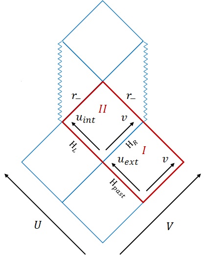 Figure 1
Peer Reviews
No public reviews on file for this paper yet. If you reviewed it on a platform where reviews are public (OpenReview, ICLR, NeurIPS, ICML), you can paste yours below so the community can read it here.
Videos
No videos yet. Explain this paper in a talk, walkthrough, or lecture? Add one.
Quantum effects near the Cauchy horizon of a Reissner-Nordström black
hole
Orr Sela
Department of physics, Technion-Israel Institute of Technology, Haifa 32000, Israel
Abstract
We consider a massless, minimally-coupled quantum scalar field on a Reissner-Nordström black hole background, and we study the leading asymptotic behavior of the expectation value of the stress energy tensor operator and of near the inner horizon, in both the Unruh and the Hartle-Hawking quantum states. We find that the coefficients of the expected leading-order divergences of these expectation values vanish, indicating that the modifications of the classical geometry due to quantum vacuum effects might be weaker than expected. In addition, we calculate the leading-order divergences of and of in the Boulware state near the outer (event) horizon, and we obtain analytical expressions that correspond to previous numerical results.
I Introduction
The classical Einstein’s field equation of general relativity admits black hole (BH) solutions with internal structures that possess exotic features such as naked singularities, Cauchy horizons and bridges to other universes. However, this is an ideal picture obtained when considering a highly symmetric, isolated black hole. Two well known solutions that have this kind of nontrivial internal structure are the Reissner-Nordström (RN) solution, describing a spherically symmetric, electrically charged BH, and the Kerr solution, describing a stationary, rotating and axially-symmetric BH.
As it turns out, when one adds (classical) external matter and perturbations to the picture, the internal region of these BH solutions is highly modified and a null curvature singularity is developed in the ingoing section of the inner horizon – the Cauchy horizon. This singularity has a very interesting nature – it is a weak singularity, meaning that the metric there is continuous but not differentiable. As a result, an observer can pass through this singularity and experience a regular physical effect (such as finite tidal forces). This phenomenon has been shown to occur for both (four dimensional) spherical charged black holes cl sing scbh 1 ; cl sing scbh 2 ; cl sing scbh 3 and rotating black holes cl sing rbh 1 ; cl sing rbh 2 ; cl sing rbh 3 ; cl sing rbh 4 . Moreover, this picture is qualitatively the same both for a test-field analysis and for an analysis that takes into account the back-reaction of the perturbations. Recently, it was shown that even on the outgoing section of the inner horizon an interesting singularity is developed – a shock-wave singularity Marolf =000026 Ori ; Eilon =000026 Ori .
In addition to these classical effects, a very important source for stress-energy (and as a result for back-reaction) is the quantum nature of fields. As Hawking Hawking 1 ; Hawking 2 showed, considering quantum fields on a (classical) BH background might result in a significant effect on the geometry (at least if taken for long enough time) and change one’s qualitative picture of this spacetime. In particular, he showed that a BH should evaporate through an emission of radiation, and therefore the entire structure of this BH spacetime turns out to be very different than the one proposed by the classical picture.
In this paper, we aim at investigating the stress-energy resulting from quantum fields in the interior region of a BH with a nontrivial internal structure (as discussed above). Specifically, we are interested in the behavior of the stress-energy tensor near the Cauchy horizon, where it is expected to diverge Birrell =000026 Davies paper ; Hiscock ; Ottewill =000026 Winstanley . Analyzing this divergence can provide us an important insight into the possible modification of the interior geometry caused by the quantum theory.
We consider the framework of semiclassical general relativity, in which the gravitational field is treated classically as a curvature of spacetime, while all the other fields are taken as quantum fields residing in this background. Therefore, instead of the classical Einstein’s field equation, we now have the following:
[TABLE]
where is the Einstein tensor of the background geometry and is the renormalized expectation value of the stress-energy tensor operator associated with the quantum fields. In Eq. (1) and throughout this paper we adopt standard geometric units and the signature .
In Ref. Birrell =000026 Davies paper , it was shown that the renormalized stress-energy tensor (RSET), calculated in the Hartle-Hawking state on a two dimensional RN black hole background, diverges at the inner horizon. Then, it was claimed that also in four dimensions the RSET is expected to diverge at the inner horizon. However, this divergence was only claimed on general grounds, without any actual calculation.
In Refs. Hiscock ; Ottewill =000026 Winstanley , it was shown that the RSET, calculated in the Unruh state on a four dimensional RN black hole background, must diverge on at least one of the two inner horizons. It was also shown that this result applies to slowly rotating black holes as well under the assumption that some components of the RSET are continuous functions of , the Kerr angular momentum parameter. A stronger assumption, that of analyticity in , yields this divergence for a general value of . This divergence, in turn, suggests that the classical picture is strongly modified by quantum vacuum effects associated with the Hawking evaporation process. However, as in Birrell =000026 Davies paper , the form of this divergence was not found.
Our goal in this work is to analyze these expected divergences at the inner horizons of black holes with a nontrivial internal structure. For this purpose, we consider a simple model with the above mentioned features: A massless, minimally coupled quantum scalar field on a RN black hole background. Being massless and minimally coupled, the scalar field operator satisfies the d’alembertian equation:
[TABLE]
where the metric used in the calculation of this d’alembertian is the RN metric. Then, after finding the asymptotic form (near the inner horizon) of the scalar field modes involved in the expression for the RSET, we calculate the expected leading-order divergence of this RSET near the inner horizon and show that its coefficient vanishes. This, in turn, suggests that the modification of the geometry might be weaker than expected. Our logic is based on experience from investigating two dimensional black hole models, where the asymptotic form of the RSET near the inner horizon determines the modification of the geometry there, even when back-reaction is taken into account Amos 2d .
An important point in our calculation of the asymptotic form of the modes near the inner horizon is that the large- limit is taken, where is the usual number appearing in the angular decomposition of the modes into spherical harmonics. That is, we assume that the leading-order behavior of and near the inner horizon is determined by the large- modes. In the external region of the BH, this assumption turns out to yield the exact asymptotic form of the RSET near the outer horizon numerically computed in Anderson ; Anderson phi2 , and in the internal region it is consistent with the numerical results of Letter that will be published elsewhere (see below for more details). For other approximation schemes which have been employed in different cases than the one considered in this paper, see Huang for an approximation of the RSET of a conformally coupled scalar field on a RN background, and Frolov ; Anderson 1 ; Anderson 2 ; Zannias for related discussions. See also Anderson ; Trace anomaly .
The organization of this paper is as follows. We start in section II with the preliminaries needed for our analysis. Then, in section III, and before we turn to the analysis in the interior region of the BH, we apply our analytical approach to the calculation of the leading-order divergence of the RSET (and of , where is the scalar field operator)* *in Boulware state upon approaching the outer (event) horizon from outside of the BH. Later, in section IV, we review some useful results from Group , where the two-point function in the interior region was expressed in terms of a radial function (or alternatively, in terms of some inner modes) that can be analytically calculated in the asymptotic region near the inner horizon. Then, in section V, we find this asymptotic form of the radial function and use it to calculate in section VI the leading divergence of and near the inner horizon. We finally conclude in section VII.
II Preliminaries
II.1 Coordinate systems and quantum states
In this paper we consider the Reissner-Nordström spacetime, which in the standard Schwarzschild coordinates has the following metric:
[TABLE]
We define the various choices of coordinates on this space following Group . First, we define the tortoise coordinate, , using the standard relation
[TABLE]
We use this relation to define both in the interior and the exterior regions of the BH. More explicitly, we choose the integration constants such that is given by
[TABLE]
in both regions, where are the surface gravities of the BH corresponding to the inner and outer horizons, and are defined as
[TABLE]
Notice that both and are chosen to be positive. Using Eq. (3), it is easy to see that the outer horizon (at ) corresponds to (both for defined in the exterior region and for that defined in the interior) and the inner horizon (at ) to .
Next, we define the Eddington-Finkelstein coordinates in the exterior region by
[TABLE]
while in the interior region by
[TABLE]
see Fig. (1). The Kruskal coordinates corresponding to the event horizon, , are defined in terms of the exterior and interior Eddington-Finkelstein coordinates by
[TABLE]
Note that we are interested in regions I and II of Fig. (1) [i.e. the region ], in which the coordinate is well defined and so we do not need to introduce different coordinates, and , for the exterior and interior regions.
We make the following notations: denotes the past horizon [i.e. the region ], PNI denotes past-null-infinity [i.e. ], is the region and is the region , see Fig. (1). We call and the “left event horizon” and “right event horizon”, respectively.
Let us now define the three quantum states that we consider in this paper. Again, we follow the notations of Group . We begin with defining the Boulware state Boulware which is defined in the exterior region of the BH. In order to do so, we decompose our (massless, minimally coupled) scalar field operator in the exterior region using two independent sets of modes , known as the Boulware modes, where denotes “in” and “up”. The decomposition is given by
[TABLE]
and the Boulware modes are defined as follows. First, these modes are solutions of the d’alembertian equation satisfied by the scalar field operator [see Eq. (2)], i.e.
[TABLE]
Exploiting the spherical symmetry, we can decompose as
[TABLE]
where
[TABLE]
and get a two-dimensional wave equation for :
[TABLE]
where
[TABLE]
The Boulware modes are then defined by demanding that are the solutions of Eq. (9) that satisfy the following initial conditions:
[TABLE]
[TABLE]
The Boulware state, , is then defined by
[TABLE]
Note that these modes and quantum state are defined in the exterior region of the BH [region I of Fig. (1)]. This state corresponds to the familiar concept of an empty state at spatial infinity, in the sense that the expectation value of the stress-energy tensor (in asymptotically Lorentzian coordinate system) in this state goes to zero at large radii Candelas . Moreover, this expectation value, evaluated in a freely falling frame, diverges at the event horizons.
An alternative and natural name for the Boulware modes that we will use in this paper is the “outer Eddington-Finkelstein modes”. Analogously to the definition of these modes, we can also define “inner Eddington-Finkelstein modes”. We shall use a similar notation for these modes, and [related by Eq. (7)], but with denoting “right” () and “left” () instead of “in” and “up”. These modes are defined in the interior region of the BH [region II of Fig. (1)] by the following initial conditions on the left and right event horizons:
[TABLE]
[TABLE]
We will use these modes repeatedly later in the paper. Note, however, that we do not involve these modes in a definition of a quantum state.
Let us now turn to the definition of the Unruh state Unruh . The field operator is decomposed as in Eq. (5) and the modes [satisfying Eq. (6)] as in Eq. (7). Everything remains the same except for the initial conditions for the modes (where we use the letter for the Unruh modes) that now take the form
[TABLE]
and
[TABLE]
Using the decomposition (5) but with the Unruh modes defined above, the Unruh state is defined as in Eq. (13). Explicitly, if we decompose the scalar field operator as
[TABLE]
the Unruh state is defined by
[TABLE]
Notice that the Unruh modes (and quantum state) are defined both in the interior and the exterior regions of the BH [regions I and II of Fig. (1)].
In Unruh state, the expectation value of the stress-energy tensor corresponds to the Hawking radiation at infinity and it is regular, in a freely falling frame, on the future event horizon but not on the past horizon Candelas .
Finally, the third quantum state that we consider is the Hartle-Hawking state Hartle =000026 Hawking . It is usually defined by an analytic continuation to the Euclidean sector, but we will mainly be interested in the mode structure of the state, as we used above for the Unruh and Boulware states. In fact, we shall be interested in known mode-sum expressions for various expectation values at the Hartle-Hawking state and will not need to use the precise form of the modes themselves, see below. The expectation value of the stress-energy tensor in Hartle-Hawking state corresponds to a thermal bath of radiation at infinity and it is regular, in a freely falling frame, on both of the event horizons Candelas .
This state is denoted by .
II.2 Regularization and Renormalization
In this paper, we consider two kinds of composite operators, and , which are quadratic in the scalar field operator and its derivatives. As is well known, composite operators formally contain divergences and need to be renormalized in order to yield a well-defined quantity. In this paper, we follow the renormalization procedure initiated by Candelas in Candelas and recently further analyzed (and generalized to a much larger extent) in Adam phi2 t ; Adam phi2 theta ; Adam T 1 ; Adam T 2 . This procedure is based on the so called point-splitting method. We begin this subsection with briefly reviewing the point-splitting method and then continue with a description of the pragmatic renormalization procedure used in this paper.
II.2.1 Point-Splitting
When dealing with composite operators which are quadratic in the field operator and its derivatives, an intuitive way to regularize these operators is to “split” the point to two distinct points and , and consider the operator which is the product of the two constituent operators at the two different points. This operator is obviously well-defined. Next, we can subtract a counterterm that removes the singularity and take the coincidence limit , thereby obtaining the renormalized operator. This is the so called point-splitting method. An essential property of the counterterm is that it is a local geometric quantity that fully captures the singular piece. In other words, it is independent of the quantum state (and therefore we can write the renormalization as an operator equation). Moreover, note that if we consider the vacuum expectation value of the split operator, we get the standard two-point function.
In Refs. Christensen 76 ; Christensen 78 , Christensen used the DeWitt-Schwinger expansion of the Feynman Green’s function Schwinger ; DeWitt (see also Birrell =000026 Davies ) to obtain the counterterms needed for the renormalization of and in the point-splitting method. In the case of , the result is
[TABLE]
where is known as the DeWitt-Schwinger counterterm, which for a scalar field with mass and coupling constant takes the form Christensen 76 ; Anderson
[TABLE]
Here, is the biscalar of geodetic separation (also known as Synge’s world function) which is equal to one-half of the square of the geodesic distance between and , is the Euler constant and and are the Ricci tensor and scalar, respectively. The parameter is not uniquely fixed and corresponds to the well-known ambiguity in the renormalization procedure.
For the stress-energy tensor, the procedure is analogous and we have
[TABLE]
where is the corresponding counterterm, which again is a local geometric quantity built from and the metric. In Christensen’s original prescription Christensen 78 , the expression , to which we may call the split stress-energy tensor, involves covariant derivatives taken at both and , along with the bi-vector of parallel transport which transfers a vector at to a vector at . In this paper, however, we use the alternative form of this prescription found in Adam T 2 . In this new form, all the derivatives in are taken at the same point , and the bi-vector of parallel transport only appears in the new form of the counterterm. This way, the derivation of the mode-sum expression for is much easier and one can naively apply the classical expressions for the stress-energy tensor for the relevant modes in order to get this mode-sum. For further discussion and the explicit form of this new counterterm , see Adam T 2 .
II.2.2 Pragmatic mode-sum renormalization method
Implementing the point-splitting renormalization is most easily done using the method introduced in Candelas ; Adam phi2 t ; Adam phi2 theta ; Adam T 1 ; Adam T 2 . In this method, we first use the mode decomposition of the field operator in order to get a mode-sum expression for the split operator (e.g. the two-point function in the case of