Applications of Psychological Science for Actionable Analytics
Di Chen, Wei Fu, Rahul Krishna, Tim Menzies

TL;DR
This paper demonstrates that Fast-and-Frugal Trees (FFTs), simple and psychologically-inspired models, outperform complex defect prediction algorithms in software analytics, especially with operational data, highlighting the value of psychological insights and simple baselines.
Contribution
The study introduces FFTs into software analytics, showing their effectiveness and advocating for psychological science-inspired models and simple baselines in the field.
Findings
FFTs are very succinct, with models of 5 lines or less.
FFTs outperform state-of-the-art defect prediction algorithms.
FFTs perform significantly better when trained on operational attributes.
Abstract
Actionable analytics are those that humans can understand, and operationalize. What kind of data mining models generate such actionable analytics? According to psychological scientists, humans understand models that most match their own internal models, which they characterize as lists of "heuristic" (i.e., lists of very succinct rules). One such heuristic rule generator is the Fast-and-Frugal Trees (FFT) preferred by psychological scientists. Despite their successful use in many applied domains, FFTs have not been applied in software analytics. Accordingly, this paper assesses FFTs for software analytics. We find that FFTs are remarkably effective. Their models are very succinct (5 lines or less describing a binary decision tree). These succinct models outperform state-of-the-art defect prediction algorithms defined by Ghortra et al. at ICSE'15. Also, when we restrict training data…
Click any figure to enlarge with its caption.
_img_FFT-R-Demo.jpg) Figure 1
_img_Popt_example.jpg) Figure 2
_img_change_freq.png) Figure 3
_img_combined.png) Figure 4
_img_combined_new.jpeg) Figure 5
_img_combined_small.jpeg) Figure 6
_img_d2h_fig.png) Figure 7
_img_d2h_heatmap.png) Figure 8
_img_d2hpopt.png) Figure 9
_img_deltas-v2.png) Figure 10
_img_deltas.png) Figure 11
_img_dist2heaven.png) Figure 12
_img_fft-demo.jpg) Figure 13
_img_fft-demo.png) Figure 14
_img_fft-frequency.png) Figure 15
_img_fft_heatmap.png) Figure 16
_img_loc_fig.png) Figure 17
_img_p_opt.png) Figure 18
_img_p_opt_demo.png) Figure 19
_img_p_opt_heatmap.png) Figure 20
_img_pair_compare.png) Figure 21
_img_pair_compare_0.png) Figure 22
_img_pair_compare_1.png) Figure 23
_img_structures.png) Figure 24
_img_trade_off.png) Figure 25
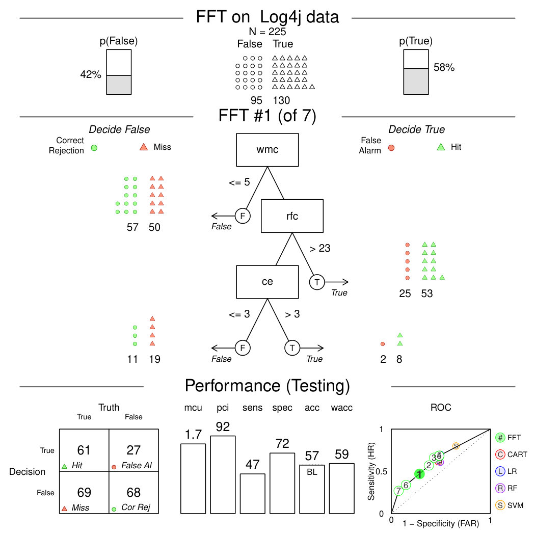 Figure 26
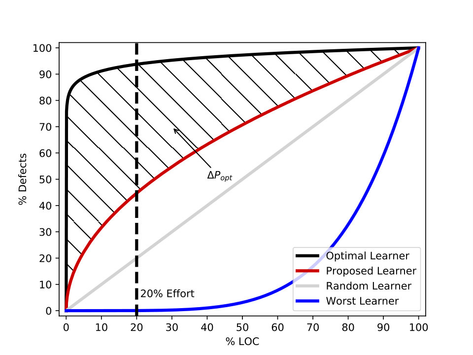 Figure 27
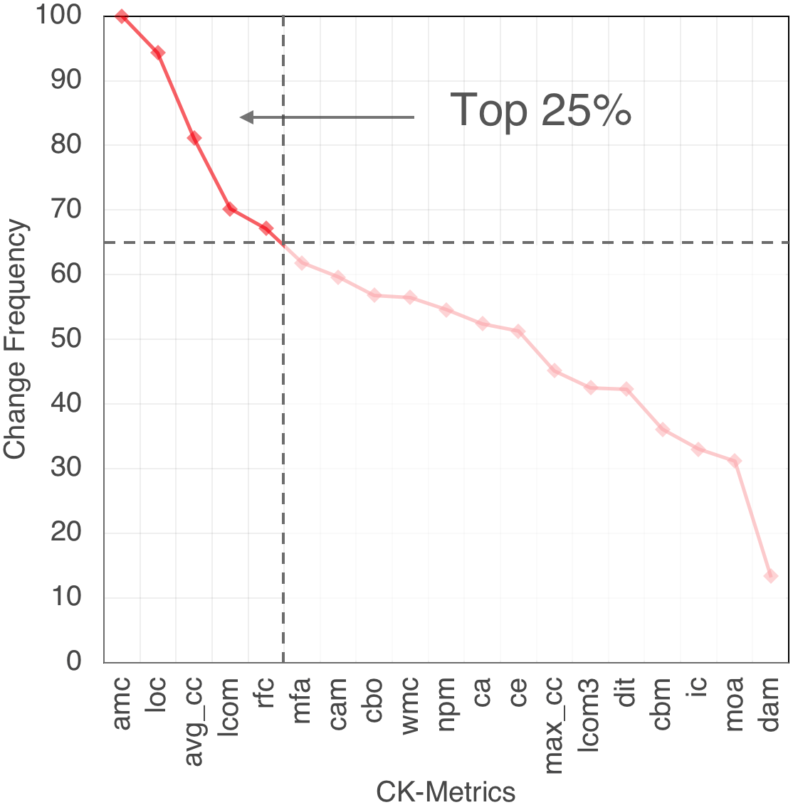 Figure 28
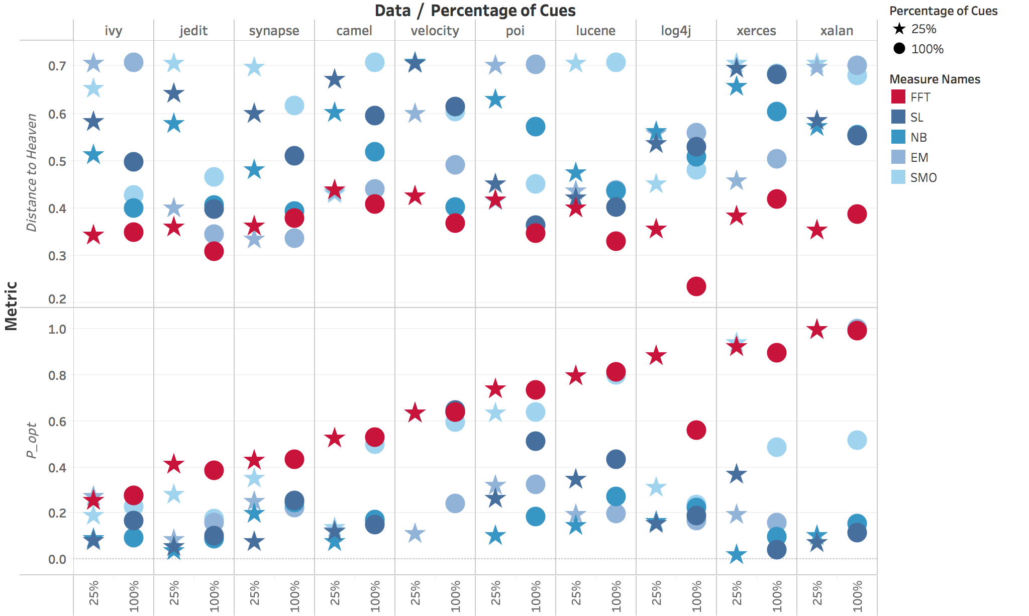 Figure 29
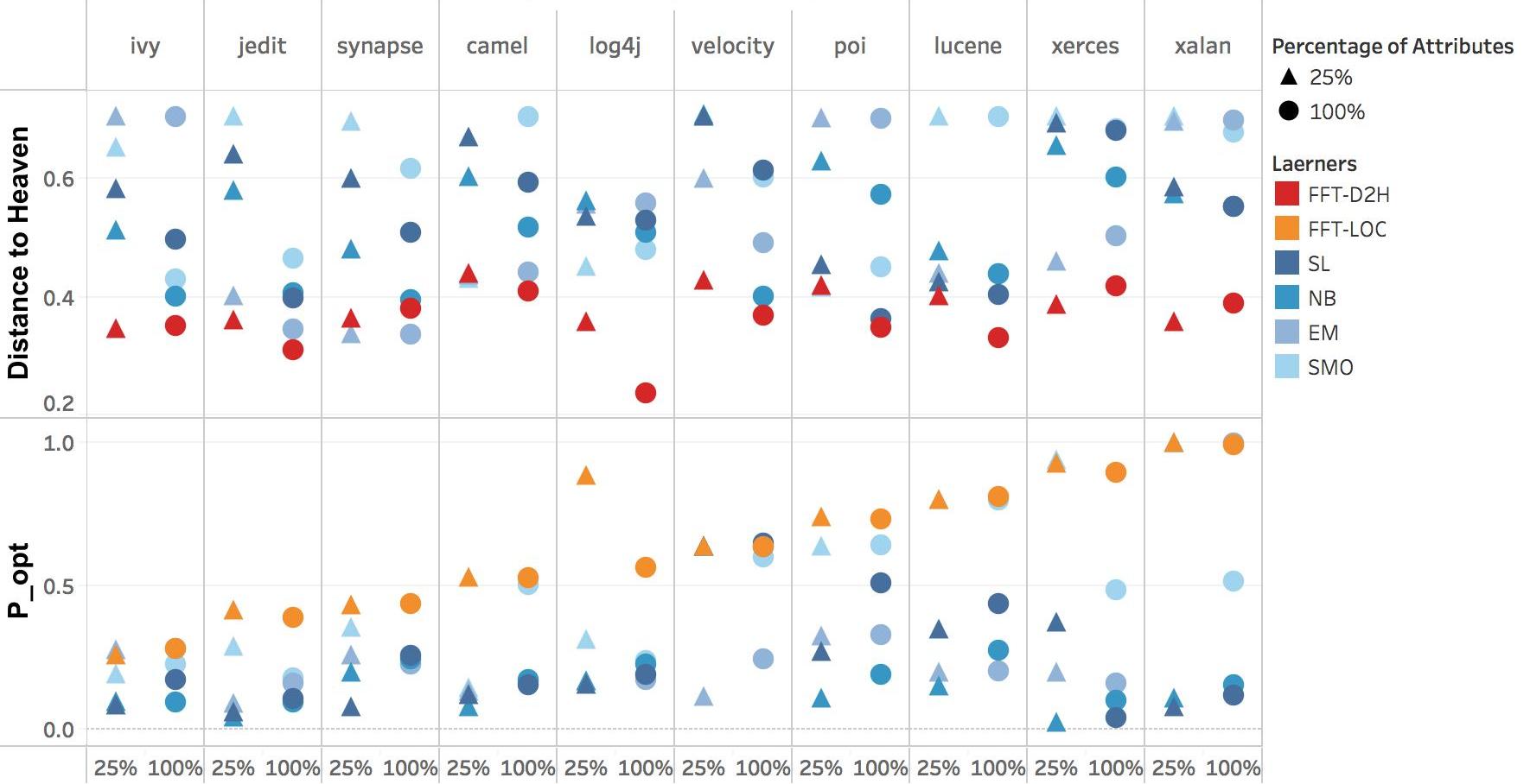 Figure 30
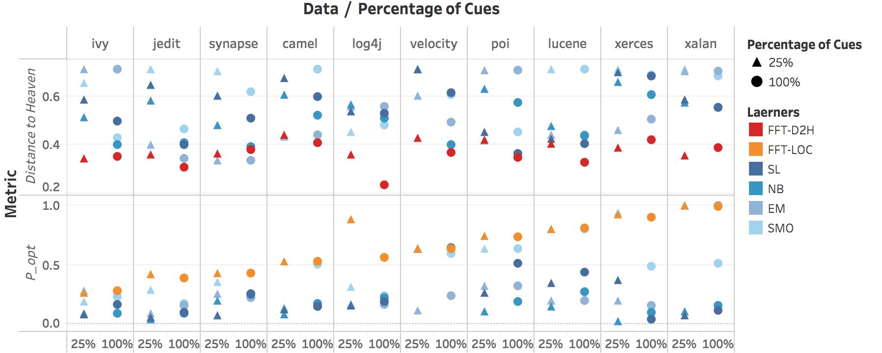 Figure 31
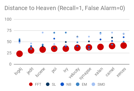 Figure 32
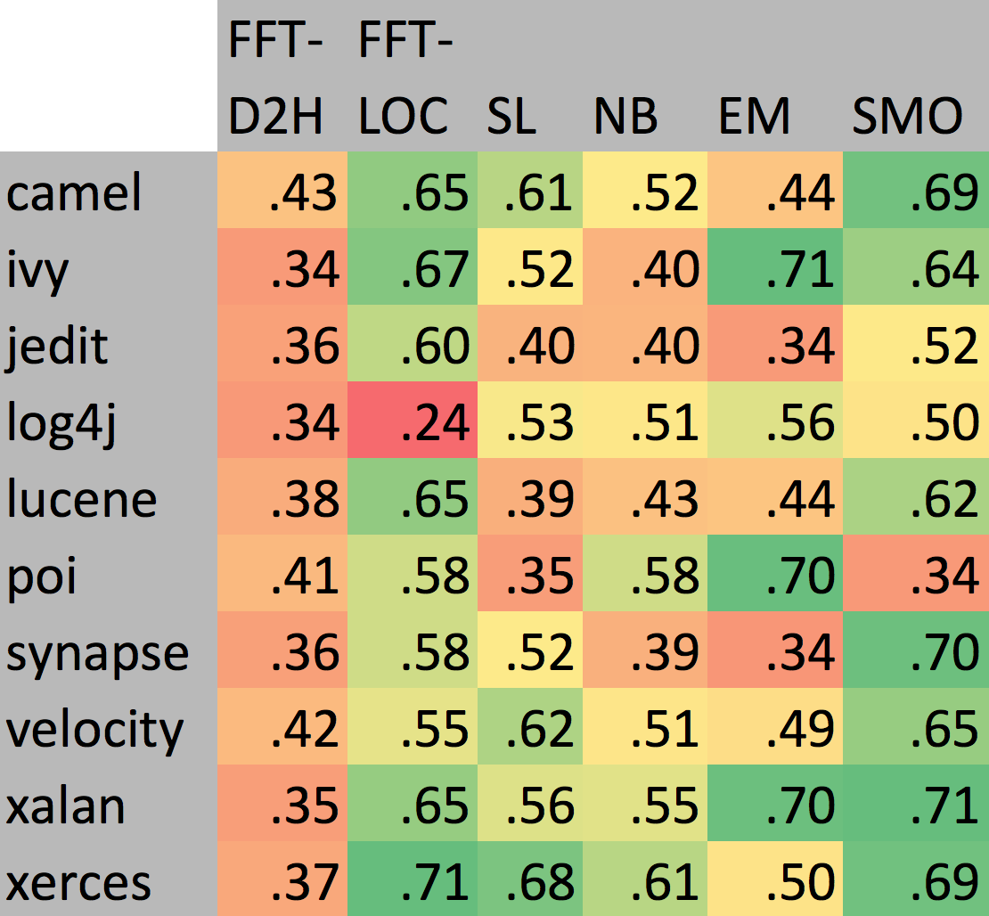 Figure 33
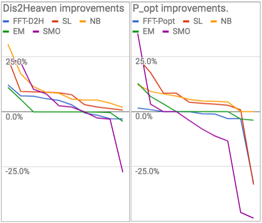 Figure 34
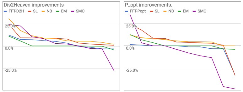 Figure 35
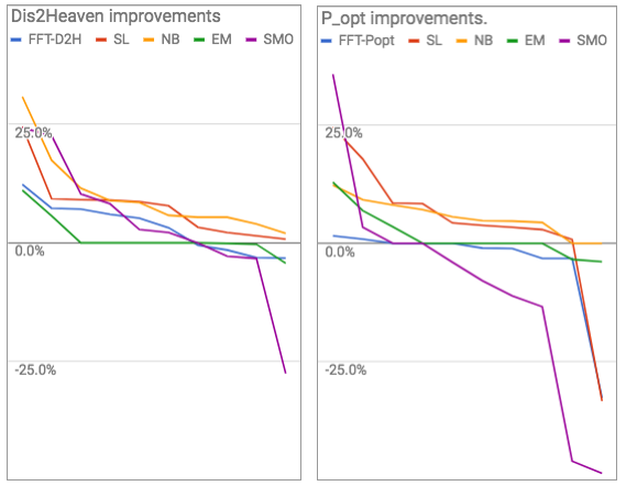 Figure 36
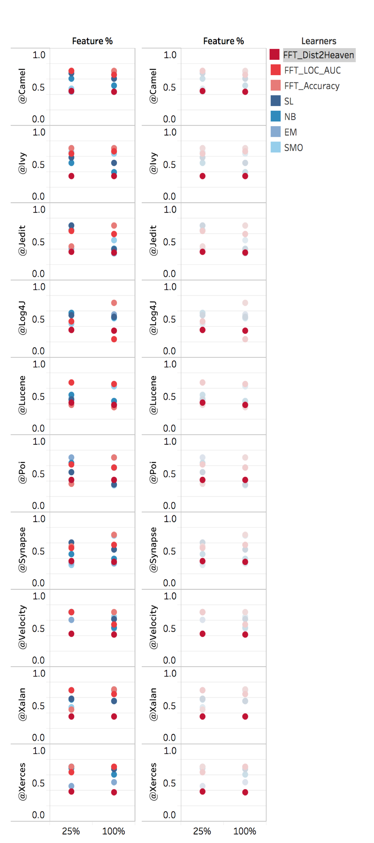 Figure 37
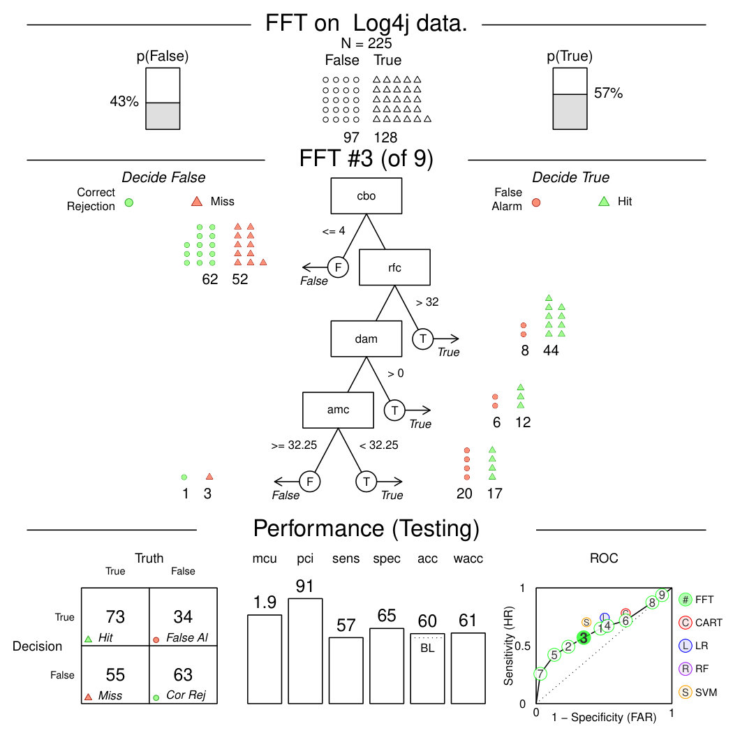 Figure 38
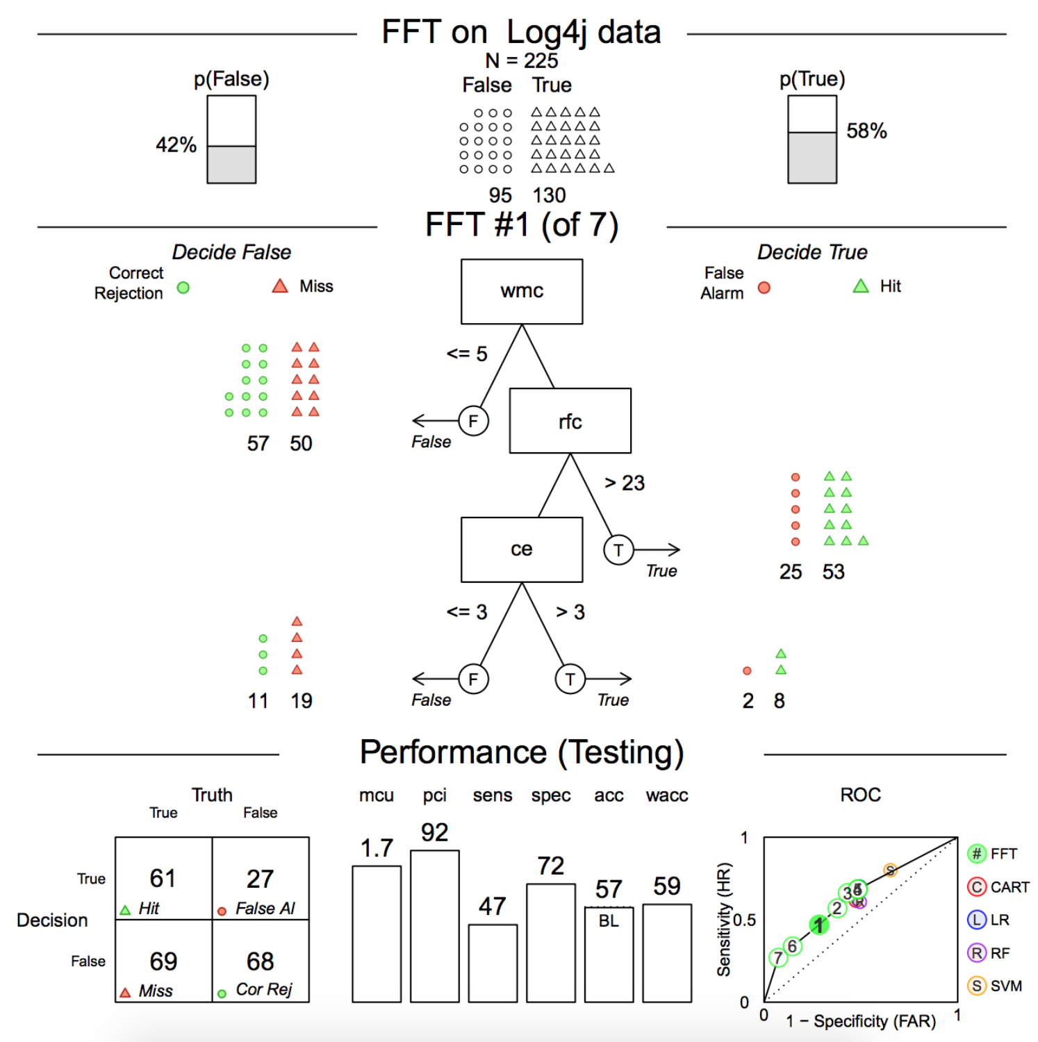 Figure 39
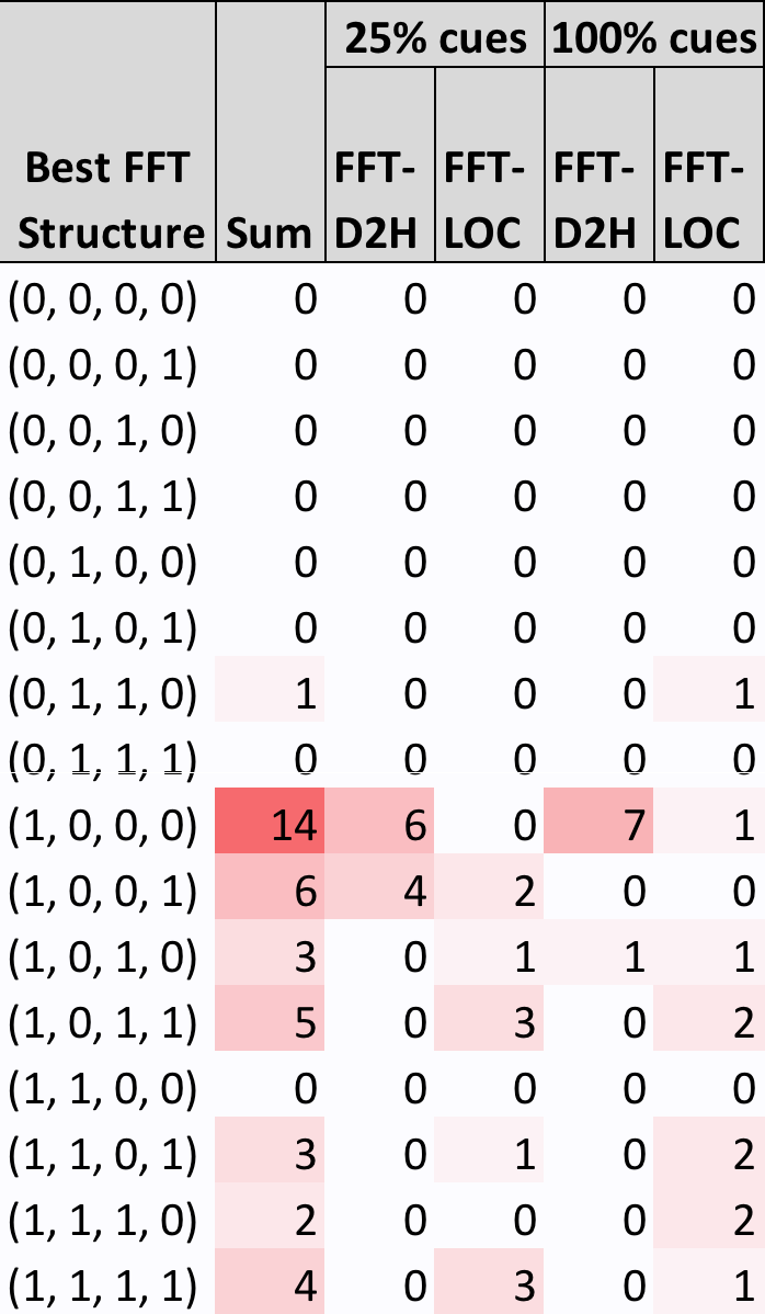 Figure 40
| Metric | Name | Description |
|---|---|---|
| amc | average method complexity | Number of JAVA byte codes |
| avg_cc | average McCabe | Average McCabe’s cyclomatic complexity seen in class |
| ca | afferent couplings | How many other classes use the specific class. |
| cam | cohesion amongst classes | Summation of number of different types of method parameters in every method divided by a multiplication of number of different method parameter types in whole class and number of methods. |
| cbm | coupling between methods | Total number of new/redefined methods to which all the inherited methods are coupled |
| cbo | coupling between objects | Increased when the methods of one class access services of another. |
| ce | efferent couplings | How many other classes is used by the specific class. |
| dam | data access | Ratio of private (protected) attributes to total attributes |
| dit | depth of inheritance tree | It’s defined as the maximum length from the node to the root of the tree |
| ic | inheritance coupling | Number of parent classes to which a given class is coupled (includes counts of methods and variables inherited) |
| lcom | lack of cohesion in methods | Number of pairs of methods that do not share a reference to an instance variable. |
| locm3 | another lack of cohesion measure | If are the number of in a class number and is the number of methods accessing an attribute, then . |
| loc | lines of code | Total lines of code in this file or package. |
| max_cc | Maximum McCabe | maximum McCabe’s cyclomatic complexity seen in class |
| mfa | functional abstraction | Number of methods inherited by a class plus number of methods accessible by member methods of the class |
| moa | aggregation | Count of the number of data declarations (class fields) whose types are user defined classes |
| noc | number of children | Number of direct descendants (subclasses) for each class |
| npm | number of public methods | npm metric simply counts all the methods in a class that are declared as public. |
| rfc | response for a class | Number of methods invoked in response to a message to the object. |
| wmc | weighted methods per class | A class with more member functions than its peers is considered to be more complex and therefore more error prone |
| defect | defect | Boolean: where defects found in post-release bug-tracking systems. |
| Training | Testing | ||||
|---|---|---|---|---|---|
| Data Set | Versions | Cases | Versions | Cases | % Defective |
| jedit | 3.2, 4.0, 4.1, 4.2 | 1257 | 4.3 | 492 | 2 |
| ivy | 1.1, 1.4 | 352 | 2.0 | 352 | 11 |
| camel | 1.0, 1.2, 1.4 | 1819 | 1.6 | 965 | 19 |
| synapse | 1.0, 1.1 | 379 | 1.2 | 256 | 34 |
| velocity | 1.4, 1.5 | 410 | 1.6 | 229 | 34 |
| lucene | 2.0, 2.2 | 442 | 2.4 | 340 | 59 |
| poi | 1.5, 2, 2.5 | 936 | 3.0 | 442 | 64 |
| xerces | 1.0, 1.2, 1.3 | 1055 | 1.4 | 588 | 74 |
| log4j | 1.0, 1.1 | 244 | 1.2 | 205 | 92 |
| xalan | 2.4, 2.5, 2.6 | 2411 | 2.7 | 909 | 99 |
| (1) First discretize all attributes; e.g., split numerics on median value. |
| (2) For each discretized range, find what rows it selects in the training data. Using those rows, score each range using some user-supplied function e.g., recall, false alarm, or the defined in §3.4. |
| (3) Divide the data on the best range. |
| (4) If the exit policy at this level is (0,1), then exit to (false,true) using the range that scores highest assuming that the target class is (false,true), respectively. |
| (5) If the current level is at , add one last exit node predicting the opposite to step 4. Then terminate. |
| (6) Else, take the data selected by the non-exit range and go to step1 to build the next level of the tree. |
| For very high dimensional data, there is some evidence that complex deep learning algorithms have advantages for software engineering applications (Yang et al., 2015; White et al., 2015; Gu et al., 2016). However, since they do not readily support explainability, they have been criticizing as “data mining alchemy” (Synced, 2017). |
| Support vector machines and principle component methods achieve their results after synthesizing new dimensions which are totally unfamiliar to human users (Menzies et al., 2009). |
| Other methods that are heavily based on mathematics can be hard to explain to most users. For example, in our experience, it is hard for (e.g.,) users to determine minimal changes to a project that mostly affect defect-proneness, just by browsing the internal frequency tables of a Naive Bayes classifier or the coefficients found via linear regression/logistic regression (Menzies et al., 2009). |
| When decision tree learners are many pages long, they are hard to browse and understand (Friedl and Brodley, 1997). |
| Random forests are even harder to understand than decision trees since the problems of reading one tree are multiplied times, one for each member of the forest (Liaw et al., 2002). |
| Instance-based methods do not compress their training data; instead they produce conclusions by finding older exemplars closest to the new example. Hence, for such instance-based methods, it is hard to generalize and make a conclusion about what kind of future projects might be (e.g.,) most defective-prone (Aha et al., 1991). |
| Commit | Comment | Issue |
|---|---|---|
| nCommitsByActorsT | meanCommentSizeT | issueCleanedBodyLen |
| nCommitsByCreator | nComments | nIssuesByCreator |
| nCommitsByUniqueActorsT | nIssuesByCreatorClosed | |
| nCommitsInProject | nIssuesCreatedInProject | |
| nCommitsProjectT | nIssuesCreatedInProjectClosed | |
| nIssuesCreatedProjectClosedT | ||
| nIssuesCreatedProjectT | ||
| Misc. | nActors, nLabels, nSubscribedByT | |
|
|
|
|
|
||||||||||
|---|---|---|---|---|---|---|---|---|---|---|---|---|---|---|
| 1 |
|
1.7 | 1.63 | 0.33 | ||||||||||
| 2 |
|
2.8 | 2.84 | 0.41 | ||||||||||
| 3 |
|
5.1 | 5.13 | 0.46 | ||||||||||
| 4 |
|
6.5 | 6.45 | 0.25 |
| Best FFF | 25% | 100% | |||
|---|---|---|---|---|---|
| exit policy | D2H | D2H | |||
| 00001 | 0 | 0 | 0 | 0 | 0 |
| 00010 | 0 | 0 | 0 | 0 | 0 |
| 00101 | 0 | 0 | 0 | 0 | 0 |
| 00110 | 0 | 0 | 0 | 0 | 0 |
| 01001 | 0 | 0 | 0 | 0 | 0 |
| 01010 | 0 | 0 | 0 | 0 | 0 |
| 01101 | 1 | 0 | 0 | 0 | 1 |
| 01110 | 0 | 0 | 0 | 0 | 0 |
| 10001 | 14 | 6 | 0 | 7 | 1 |
| 10010 | 8 | 4 | 2 | 2 | 0 |
| 10101 | 3 | 0 | 1 | 1 | 1 |
| 10110 | 5 | 0 | 3 | 0 | 2 |
| 11001 | 0 | 0 | 0 | 0 | 0 |
| 11010 | 3 | 0 | 1 | 0 | 2 |
| 11101 | 2 | 0 | 0 | 0 | 2 |
| 11110 | 4 | 0 | 3 | 0 | 1 |
| Totals | 40 | 10 | 10 | 10 | 10 |
| Days till closed | |||||||
|---|---|---|---|---|---|---|---|
| Data(# of instances) | |||||||
| cloudstack (1551) | FFT | FFT | FFT | FFT | FFT | DT | LR |
| node (6207) | FFT | FFT | FFT | FFT | FFT | DT | LR |
| deeplearning (1434) | FFT | FFT | FFT | FFT | FFT | FFT | RF |
| cocoon (2045) | FFT | FFT | FFT | FFT | FFT | FFT | FFT |
| ofbiz (6177) | FFT | FFT | FFT | FFT | FFT | FFT | FFT |
| camel (5056) | RF/KNN | KNN | FFT/KNN/DT | FFT | FFT | FFT | FFT |
| hadoop (12191) | KNN | DT | DT | FFT | FFT | FFT | FFT |
| qpid (5475) | DT | DT/RF | DT | FFT | FFT | FFT | FFT |
Peer Reviews
No public reviews on file for this paper yet. If you reviewed it on a platform where reviews are public (OpenReview, ICLR, NeurIPS, ICML), you can paste yours below so the community can read it here.
Videos
No videos yet. Explain this paper in a talk, walkthrough, or lecture? Add one.
Taxonomy
TopicsSoftware Engineering Research · Software Reliability and Analysis Research · Software Engineering Techniques and Practices
Applications of Psychological Science for Actionable Analytics
Di Chen, Wei Fu, Rahul Krishna, Tim Menzies
North Carolina State University, USARaleighNC27606
dchen20, wfu, [email protected], [email protected]
(2018)
Abstract.
Actionable analytics are those that humans can understand, and operationalize. What kind of data mining models generate such actionable analytics? According to psychological scientists, humans understand models that most match their own internal models, which they characterize as lists of “heuristic” (i.e., lists of very succinct rules). One such heuristic rule generator is the Fast-and-Frugal Trees (FFT) preferred by psychological scientists. Despite their successful use in many applied domains, FFTs have not been applied in software analytics. Accordingly, this paper assesses FFTs for software analytics.
We find that FFTs are remarkably effective. Their models are very succinct (5 lines or less describing a binary decision tree). These succinct models outperform state-of-the-art defect prediction algorithms defined by Ghortra et al. at ICSE’15. Also, when we restrict training data to operational attributes (i.e., those attributes that are frequently changed by developers), FFTs perform much better than standard learners.
Our conclusions are two-fold. Firstly, there is much that software analytics community could learn from psychological science. Secondly, proponents of complex methods should always baseline those methods against simpler alternatives. For example, FFTs could be used as a standard baseline learner against which other software analytics tools are compared.
Decision trees, heuristics, software analytics, psychological science, empirical studies, defect prediction
††conference: 12th Joint Meeting of the European Software Engineering Conference and the ACM SIGSOFT Symposium on the Foundations of Software Engineering; 4–9 November, 2018; Lake Buena Vista, Florida††copyright: rightsretained††doi: XX.YY/ZZ††isbn: ZZ-YY-24-ZZ/QQ/A††conference: Florida; Nov 2018; ††journalyear: 2018††price: 15.00††submissionid: 123-A12-B3
1. Introduction
Data mining tools have been applied to many applications in Software Engineering (SE). For example, it has been used to estimate how long it would take to integrate new code into an existing project (Czerwonka et al., 2011), where defects are most likely to occur (Ostrand et al., 2004; Menzies et al., 2007a), or how long will it take to develop a project (Turhan et al., 2011; Kocaguneli et al., 2012), etc. Large organizations like Microsoft routinely practice data-driven policy development where organizational policies are learned from an extensive analysis of large datasets (Begel and Zimmermann, 2014; Theisen et al., 2015).
Despite these successes, there exists some drawbacks with current software analytic tools. At a recent workshop on “Actionable Analytics” at ASE’15, business users were very vocal in their complaints about analytics (Hihn and Menzies, 2015), saying that there are rarely producible models that business users can understand or operationalize.
Accordingly, this paper explores methods for generating actionable analytics for:
- •
Software defect prediction;
- •
Predicting close time for Github issues.
There are many ways to define “actionable” but at the very least, we say that something is actionable if people can read and use the models it generates. Hence, for this paper, we assume:
Actionable = Comprehensible + Operational.
We show here that many algorithms used in software analytics generate models that are not actionable. Further, a data mining algorithm taken from psychological science (Czerlinski et al., 1999; Gigerenzer et al., 1999; Martignon et al., 2003; Brighton, 2006; Martignon et al., 2008; Gigerenzer, 2008; Gigerenzer and Gaissmaier, 2011; Neth and Gigerenzer, 2015), called Fast-and-Frugal trees (FFTs111The reader might be aware that FFT is also an acronym for “Fast Fourier Transform”. Apparently, the psychological science community was unaware of that acronym when they named this algorithm.), are very actionable.
Note that demanding that analytics be actionable also imposes certain restrictions on (a) the kinds of models that can be generated and (b) the data used to build the models.
- (a)
Drawing on psychological science, we say an automatically generated model is comprehensible if:
- –
The model matches the models used internally by humans; i.e., it comprises small rules.
- –
Further, for expert-level comprehension, the rules should quickly lead to decisions (thus freeing up memory for other tasks).
For more on this point, see Section 2.2.
- (b)
As to operational, we show in the historical log of software projects that only a few of the measurable project attributes are often changed by developers. For a data mining algorithm to be operational, it must generate effective models even if restricted to using just those changed attributes.
Using three research questions, this paper tests if these restrictions damage our ability to build useful models.
RQ1: Do FFTs models perform worse than the current state-of-the-art? We will find that:
{bclogo}
[couleur=gray!20,arrondi=0.1,logo=\bctrombone,ombre=true] For defect prediction, FFTs out-perform the state-of-art. When compared to state-of-the-art defect prediction algorithms surveyed by Ghotra et al. (Ghotra et al., 2015), FFTs are more effective (where “effective” is measured in terms of a recall/false alarm metric or the metric defined in § 3.4).
RQ2: Are FFTs more operational than the current state-of-the-art? This research question tests what happens when we learn from less data; i.e., if we demand our models avoid using attributes that are rarely changed by developers. We show that:
{bclogo}
[couleur=gray!20,arrondi=0.1,logo=\bctrombone,ombre=true] When learning from less data, FFTs performance is stabler than some other learners. When data is restricted to attributes that developers often change, then FFTs performance is only slightly changed while the performance of some other learners, can vary by alarmingly large amounts.
The observed superior performance of FFT raises the question:
RQ3: Why do FFTs work so well? Our answer to this question will be somewhat technical but, in summary we will say:
{bclogo}
[couleur=gray!20,arrondi=0.1,logo=\bctrombone,ombre=true] FFTs match the structure of SE data SE data divides into a few regions with very different properties and FFTs are good way to explore such data spaces.
In summary, the contributions of this paper are:
- •
A novel inter-disciplinary contribution of the application of psychological science to software analytics.
- •
A cautionary tale that, for software analytics, more complex learners can perform worse.
- •
A warning that many current results in software analytics make the, possibly unwarranted, assumption that merely because an attribute is observable, that we should use those attributes in a model.
- •
Three tests for “actionable analytics”: (a) Does a data mining produce succinct models? (b) Do those succinct models perform as well, or better, than more complex methods? (c) If the data mining algorithm is restricted to just the few attributes that developers actually change, does the resulting model perform satisfactorily?
- •
A demonstration that the restraints demanding by actionable analytics (very simple models, access to less data) need not result in models with poor performance.
- •
A new, very simple baseline data mining method (FFTs) against which more complex methods can be compared.
- •
A reproduction package containing all the data and algorithms of this paper, see http://url_blinded_for_review.
The rest of this paper is structured as follows. In Section 2, we introduce the concepts of “operational” and “comprehensible” as the preliminaries. Our data, experimentation settings and evaluation measures will be described in Section 3. In Section 4, we show our results and answer to research questions. Threats and validity of our work is given in Section 5. In Section 6, we conclude this paper with the following:
- •
There is much the software analytics community could learn from psychological science.
- •
Proponents of complex methods should always baseline those methods against simpler alternatives.
Finally, we discuss future work.
2. Preliminaries
2.1. Operational
This paper assumes that for a data mining algorithm to be operational, it must generate effective models even if restricted to using just those attributes which, in practice, developers actually change. We have two reasons for making that assumption.
Firstly, this definition of operational can make a model much more acceptable to developers. If a model says that, say, leads to defective code then developers will ask for guidance on how to reduce “x” (in order to reduce the chances of defects). If we define “operational” as per this article, then it is very simple matter to offer that developer numerous examples, from their own project’s historical log, of how “x” was changed.
Secondly, as shown in Figure 1 there exist attributes that are usually not changed from one version to the next. Figure 1 is important since, as shown in our RQ2 results, when we restrict model construction to just the 25% most frequently changed attributes, this can dramatically change the behavior of some data mining algorithms (but not FFTs).
Technical aside: in Figure 1, we defined “changed” using the A12 test (Vargha and Delaney, 2000) which declares two distributions different if they differ by more than a small effect. A recent ICSE’11 article (Arcuri and Briand, 2011) endorsed the use of A12 due to its non-parametric nature, it avoids any possibly incorrect Gaussian assumptions about the data.
2.2. Comprehensible
Why Demand Comprehensibility?
This paper assumes that better data mining algorithms are better at explaining their models to humans. But is that always the case?
The obvious counter-argument is that if no human ever needs to understand our audited model, then it does not need to be comprehensible. For example, a neural net could control the carburetor of an internal combustion engine since that carburetor will never dispute the model or ask for clarification of any of its reasoning.
On the other hand, if a model is to be used to persuade software engineers to change what they are doing, it needs to be comprehensible so humans can debate the merits of its conclusions. Several researchers demand that software analytics models needs to be expressed in a simple way that is easy for software practitioners to interpret (Menzies, 2014; Lipton, 2016; Dam et al., 2018). According to Kim et al. (Kim et al., 2016), software analytics aim to obtain actionable insights from software artifacts that help practitioners accomplish tasks related to software development, systems, and users. Other researchers (Tan and Chan, 2016) argue that for software vendors, managers, developers and users, such comprehensible insights are the core deliverable of software analytics. Sawyer et al. comments that actionable insight is the key driver for businesses to invest in data analytics initiatives (Sawyer, 2013). Accordingly, much research focuses on the generation of simple models, or make blackbox models more explainable, so that human engineers can understand and appropriately trust the decisions made by software analytics models (Fu and Menzies, 2017; Abdollahi and Nasraoui, 2016).
If a model is not comprehensible, there are some explanation algorithms that might mitigate that problem. For example:
- •
In secondary learning, the examples given to a neural network are used to train a rule-based learner and those learners could be said to “explain” the neural net (Craven and Shavlik, 2014).
- •
In contrast set learning for instance-based reasoning, data is clustered and users are shown the difference between a few exemplars selected from each cluster (Krishna and Menzies, 2015).
Such explanation facilities are post-processors to the original learning method. An alternative simpler approach would be to use learners that generate comprehensible models in the first place.
The next section of this paper discusses one such alternate approach for creating simple comprehensible models.
Theories of Expert Comprehension
Psychological science argues that models comprising small rules are more comprehensible. This section outlines that argument.
Larkin et al. (Larkin et al., 1980) characterize human expertise in terms of very small short term memory, or STM (used as a temporary scratch pad for current observation) and a very large long term memory, or LTM. The LTM holds separate tiny rule fragments that explore the contents of STM to say “when you see THIS, do THAT”. When an LTM rule triggers, its consequence can rewrite STM contents which, in turn, can trigger other rules.
Short term memory is very small, perhaps even as small as four to seven items (Miller, 1956; Cowan, 2001) 222Recently, Ma et al. (Ma et al., 2014) used evidence from neuroscience and functional MRIs to argue that STM capacity might be better measured using other factors than “number of items”. But even they conceded that “the concept of a limited (STM) has considerable explanatory power for behavioral data”.. Experts are experts, says Larkin et al. (Larkin et al., 1980) because the patterns in their LTM patterns dictate what to do, without needing to pause for reflection. Novices perform worse than experts, says Larkin et al., when they fill up their STM with too many to-do’s where they plan to pause and reflect on what to do next. Since, experts post far fewer to-do’s in their STMs, they complete their tasks faster because (a) they are less encumbered by excessive reflection and (b) there is more space in their STM to reason about new information. While first proposed in 1981, this STM/LTM theory still remains relevant (Ma et al., 2014). This theory can be used to explain both expert competency and incompetency in software engineering tasks such as understanding code (Wiedenbeck et al., 1993).
Phillips et al. (Phillips et al., 2017) discuss how models containing tiny rule fragments can be quickly comprehended by doctors in emergency rooms making rapid decisions; or by soldiers on guard making snap decisions about whether to fire or not on a potential enemy; or by stockbrokers making instant decisions about buying or selling stock. That is, according to this psychological science theory (Czerlinski et al., 1999; Gigerenzer et al., 1999; Martignon et al., 2003; Brighton, 2006; Martignon et al., 2008; Gigerenzer, 2008; Phillips et al., 2017; Gigerenzer and Gaissmaier, 2011; Neth and Gigerenzer, 2015), humans best understand a model:
- •
When they can “fit” it into their LTM; i.e., when that model comprises many small rule fragments;
- •
Further, to have an expert-level comprehension of some domain meaning having rules that can very quickly lead to decisions, without clogging up memory.
Psychological scientists have developed FFTs as one way to generate comprehensible models consisting of separate tiny rules (Phillips et al., 2017; Gigerenzer, 2008; Martignon et al., 2008). A FFT is a decision tree with exactly two branches extending from each node, where either one or both branches is an exit branch leading to a leaf (Martignon et al., 2008). That is to say, in an FFT, every question posed by a node will trigger an immediate decision (so humans can read every leaf node as a separate rule).
For example, Table 2 (at left) is an FFT generated from the log4j JAVA system of Table 3. The goal of this tree is to classify a software module as “defective=true” or “defective=false”. The four nodes in this FFT reference four static code attributes cbo, rfc, dam, amc (these metrics are defined in Table 1).
FFTs are a binary classification algorithm. To apply such classifiers to mulit-classes problems: (a) build one FFTs for each class for classX or not classX; (b) run all FFTs on the test example, then (c) then select conclusion with most support (number of rows).
An FFT of depth has a choice of two “exit policies” at each level: the existing branch can select for the negation of the target (denoted “0”) or the target (denoted “1”). The left-hand-side log4j tree in Table 2 is hence an 01110 tree since:
- •
The first level exits to the negation of the target: hence, “0”.
- •
While the next tree levels exit first to target; hence, “111”.
- •
And the final line of the model exits to the opposite of the penultimate line; hence, the final “0”.
To build one FFT tree, select a maximum depth , then follow the steps described in Table 4
For trees of depth , there are possible trees which we denoted 00001, 00010, 00101,… , 11110. Here, the first four digits denote the 16 exit policies and the last digit denotes the last line of the model (which makes the opposite conclusion to the line above). For example:
- •
A “00001” tree does it all it can to avoid the target class. Only after clearing away all the non-defective examples it can at levels one, two, three, four does it make a final “true” conclusion. Table 2 (right) shows the log4j 00001 tree. Note that all the exits, except the last, are to “false”.
- •
As to “11110” trees, these fixate on finding the target. Table 2 (center) shows the log4j 11110 tree. Note that all the exits, except the last, are to “true”.
During FFT training, we generate all trees then, using the predicate , select the best one (using the training data). This single best tree is then applied to the test data.
Following the advice of (Phillips et al., 2017), for all the experiments of this paper, we use a depth . Note that FFTs of such small depths are very succinct (see above examples). Many other data mining algorithms used in software analytics are far less succinct and far less comprehensible (see Table 5).
The value of models such as FFTs comprising many small rules has been extensively studied:
- •
These models use very few attributes from the data. Hence they tend to be robust against overfitting, especially on small and noisy data, and have been found to predict data at levels comparable with regression. See for example (Martignon et al., 2008; Woike et al., 2017; Czerlinski et al., 1999).
- •
Other work has shown that these rule-based models can perform comparably well to more complex models in a range of domains e.g., public health, medical risk management, performance science, etc. (Jenny et al., 2013; Laskey and Martignon, 2014; Raab and Gigerenzer, 2015).
- •
Neth and Gigerenzer argue that such rule-bases are tools that work well under conditions of uncertainty (Neth and Gigerenzer, 2015).
- •
Brighton showed that rule-based models can perform better than complex nonlinear algorithms such as neural networks, exemplar models, and classification/regression trees (Brighton, 2006).
3. Methods
The use of models comprising many small rules has not been explored in the software analytics literature. This section describes the methods used by this paper to assess FFTs.
3.1. Data
3.1.1. Defect Data:
To assess the FFTs, we perform our experiments using the publicly available SEACRAFT data (Jureczko and Madeyski, 2010), gathered by Jureczko et al. for object-oriented JAVA systems (Jureczko and Madeyski, 2010). The “Jureczko” data records the number of known defects for each class using a post-release defect tracking system. The classes are described in terms of nearly two dozen metrics such as number of children (noc), lines of code (loc), etc (see Table 1). For details on the Jureczko data, see Table 3. The nature of collected data and its relevance to defect prediction is discussed in greater detail by Madeyski & Jureczko (Madeyski and Jureczko, 2015).
We selected these data sets since they have at least three consecutive releases (where release was built after release ). This is important for our experimental rig (see section 3.2).
3.1.2. Issue Lifetime Data:
This paper will conclude that FFTs are remarkable effective. To check the external validity of that conclusion, we will apply FFT to another SE domain (Rahul Krishna, 2018; Rees-Jones et al., 2018). Our Github issue lifetime data333https://doi.org/10.5281/zenodo.197111 consists of 8 projects used to study issue lifetimes. In raw form, the data consisted of sets of JSON files for each repository, each file contained one type of data regarding the software repository (issues, commits, code contributors, changes to specific files as shown in Table 6). In order to extract data specific to issue lifetime, we did similar preprocessing and feature extraction on the raw datasets as suggested by (Rees-Jones et al., 2018).
3.2. Experimental Rig
For the defect prediction data, we use versions of the software systems in Table 3.
Using versions , we track what attributes change by from version to (using the calculation shown in Figure 1). Then we build a model using all the attributes from version or just the top 25% most changed attributes. Note that this implements our definition of “operational”, as discussed in our introduction.
After building a model, we use the latest version for testing while the older versions for training. In this way, we can assert that all our predictions are using past date to predict the future.
For the issue lifetime data, we do not have access to multiple versions of the data. Hence, for this data we cannot perform the operational test. Hence, for that data we conduct a 5*10 cross-validation experiment that ensures that the train and test sets are different. For that cross-val, we divide the data into ten bins, then for each bin we train on then test on bin . To control for order effects (where the conclusions are altered by the order of the input examples) (Agrawal et al., 2018), this process is repeated five times, using different random orderings of the data.
3.3. Data Mining Algorithms
The results shown below compare FFTs to state of the art algorithms from software analytics. For a list of state-of-algorithms, we used the ICSE’15 paper from Ghotra et al. (Ghotra et al., 2015) which compared 32 classifiers for defect prediction. Their statistical analysis showed that the performance of these classifiers clustered into four groups shown in Table 7. For our work, we selected one classifier at random from each of their clusters: i.e., Simple Logistic (SL), Naive Bayes (NB), Expectation Maximization (EM), Sequential Minimal Optimization (SMO).
Simple Logistic and Naive Bayes falls into the 1st and 2nd rankings layers. They are both statistical techniques that are based on a probability based model (Kotsiantis et al., 2007). These techniques are used to find patterns in datasets and build diverse predictive models (Berson et al., 2004). Simple Logistic is a generalized linear regression model that uses a logit function. Naive Bayes is a probability-based technique that assumes that all of the predictors are independent of each other.
Clustering techniques like EM divide the training data into small groups such that the similarity within groups is more than across the groups (Hammouda and Karray, 2000). EM is a clustering technique based on cluster performance Expectation Maximization (Fraley and Raftery, 2007) (EM) technique, which automatically splits a dataset into an (approximately) optimal number of clusters (Bettenburg et al., 2012).
Support Vector Machines (SVMs) use a hyperplane to separate two classes (i.e., defective or not). In this paper, following the results of Ghotra et al., we use the Sequential Minimal Optimization (SMO) SVM technique. SMO analytically solves the large Quadratic Programming (QP) optimization problem which occurs in SVM training by dividing the problem into a series of possible QP problems (Zeng et al., 2008).
3.4. Evaluation Measures
Our rig assess learned models using an evaluation function called . For FFTs, this function is called three times:
- •
Once to rank discretized ranges;
- •
Then once again to select the best FFT out of the trees generated during training.
- •
Then finally, is used to score what happens when that best FFT is applied to the test data.
For all the other learners, score is applied on the test data. For this work, we use the two measures: dis2heaven and .
Ideally, a perfect learner will have perfect recall (100%) with no false alarms.
[TABLE]
[TABLE]
We combine these two into a “distance to heaven” measure called dis2heaven that reports how far a learner falls away from the ideal point of Recall=1 and FAR=0:
[TABLE]
As to , Ostrand et al. (Ostrand et al., 2005) report that their quality predictors can find 20% of the files contain on average 80% of all defects in the project. Although there is nothing magical about the number 20%, it has been used as a cutoff value to set the efforts required for the defect inspection when evaluating the defect learners (Kamei et al., 2013; Mende and Koschke, 2010; Monden et al., 2013; Yang et al., 2016). That is, reports how many defects have been found after (a) the code is sorted by the learner from “most likely to be buggy” to “least likely”; then (b) humans inspect 20% of the code (measured in lines of code), where that code has , how many defects can be detected by the learner. This measure is widely used in defect prediction literature (Kamei et al., 2013; Menzies et al., 2007c; Menzies et al., 2010; Monden et al., 2013; Yang et al., 2016; Zimmermann et al., 2007).
is defined as , where is the area between the effort cumulative lift charts of the optimal model and the prediction model (as shown in Figure2). In this chart, the x-axis is the percentage of required effort to inspect the code and the y-axis is the percentage of defects found in the selected code. In the optimal model, all the changes are sorted by the actual defect density in descending order, while for the predicted model, all the changes are sorted by the actual predicted value in descending order. According to Kamei et al. and Xu et al. (Kamei et al., 2013; Monden et al., 2013; Yang et al., 2016) can be normalized as follows:
[TABLE]
where , and represent the area of curve under the optimal model, predicted model, and worst model, respectively. This worst model is built by sorting all the changes according to the actual defect density in ascending order.
Note that for our two score functions:
- •
For dis2heaven, the lower values are better.
- •
For , the higher values are better.
4. Results
4.1. RQ1: Do FFTs models perform worse than the current state-of-the-art?
Figure 3 compares the performance of FFT versus learners taken from Ghotra et al. In this figure, datasets are sorted left right based on the FFT performance scores. With very few exceptions:
- •
FFT’s dis2heaven’s results lower, hence better, than the other learners.
- •
FFT’s results are much higher, hence better, than the other learners.
Therefore our answer to RQ1 is:
{bclogo}
[couleur=gray!20,arrondi=0.1,logo=\bctrombone,ombre=true] For defect prediction, FFTs out-perform the state-of-art. When compared to state-of-the-art defect prediction algorithms surveyed by Ghotra et al., FFTs are more effective (where “effective” is measured in terms of a recall/false alarm metric or ).
4.2. RQ2: Are FFTs more operational than the current state-of-the-art?
Please recollect from before that a model is operational if its performance is not affected after avoiding attributes that are rarely changed by developers.
Figure 4 compares model performance when we learn from all 100% attributes or just the 25% most changed attributes. For this study, these 25% group (of most changed attributes) was computed separately for each data set. Note that:
- •
The top row of Figure 4 shows the dis2heaven results;
- •
The bottom row of Figure 4 shows the results.
Figure 5 reports the deltas in performance scores seen between using 25% and 100% of the data. These deltas are computed such that larger values are better; i.e., for (dist2heaven, ) we report (25%-100%, 100%-25%) since (fewer, more) values are better (respectively).
There are several key features for these results:
- •
The FFT’s red dots for dis2heaven are below the rest; also, FFT’s orange dots for are above the rest. This means that, regardless of whether we use all attributes or just the most changed attributes, the FFT results are nearly always better than the other methods.
- •
As seen in Figure 5, the deltas between using all data and just some of the data is smallest for FFTs and EM (the instance-based clustering algorithm). In , those deltas are very small indeed (the FFT and EM results lie right on the y-axis for most of that plot).
- •
Also, see in Figure 5, the deltas on the other learners can be highly variable. While for the most part, using just the 25% most changed attributes improves performance, SMO , SL and NB all have large negative results for at least some of the data sets.
In summary, the learners studied here fall into three groups:
- (1)
Those that exhibited a wide performance variance after restricting the learning to just the frequently changed data (SL, NB, SMO), and those that are not (FFT, EM); 2. (2)
Those with best performance across the two performance measures studied here (FFT), and the rest (SL, NB, EM, SMO); 3. (3)
Those that generate tiny models (FFT), and the rest (SL, NB, EM, SMO).
Accordingly, FFT is the recommended learner since it both performs well and is unaffected by issues such as whether or not the data is restricted to just the most operational attributes. In summary:
{bclogo}
[couleur=gray!20,arrondi=0.1,logo=\bctrombone,ombre=true] When learning from less data, FFTs performance is stabler than some other learners. When data is restricted to attributes that developers often change, then FFTs performance is only slightly changed while the performance of some other learners, can vary by alarmingly large amounts.
4.3. RQ3: Why do FFTs work so well?
To explain the success of FFTs, recall that during training, FFTs explores models, then selects the models whose exit policies achieves best performances (exit policies were introduced in Section 2.2). The exit policies selected by FFTs are like a trace of the reasoning jumping around the data. For example, a 11110 policy shows a model always jumping towards sections of the data containing most defects. Also, a 00001 policy show another model trying to jump away from defects until, in its last step, it does one final jump towards defects. Table 8 shows what exit policies were seen in the experiments of the last section:
- •
The 11110 policy was used sometimes.
- •
A more common policy is 10001 which shows a tree first jumping to some low hanging fruit (see the first “1”), then jumping away from defects three times (see the next “000”) before a final jump into defects (see the last “1”).
- •
That said, while 10001 was most common, many other exit policies appear in Table 8. For example, the policies are particularly diverse.
Table 8 suggests that software data is “lumpy”; i.e., it divides into a few separate regions, each with different properties. Further, the number and importance of the “lumps” is specific to the data set and the goal criteria. In such a “lumpy” space, a learning policy like FFT works well since its exit policies let a learner discover how to best jump between the “lumps”. Other learners fail in this coarse-grained lumpy space when they:
- •
Divide the data too much; e.g. like RandomForests, which finely divide the data multiple times down the branches of the trees and across multiple trees;
- •
Fit some general model across all the different parts of the data; e.g. like simple logistic regression.
In summary, in answer to the question “why do FFTs work so well”, we reply:
{bclogo}
[couleur=gray!20,arrondi=0.1,logo=\bctrombone,ombre=true] FFTs match the structure of SE data SE data divides into a few regions with very different properties and FFTs are good way to explore such data spaces.
5. Threats to Validity
5.1. Sampling Bias
This paper shares the same sampling bias problem as every other data mining paper. Sampling bias threatens any classification experiment; what matters in one case may or may not hold in another case. For example, even though we use 10 open-source datasets in this study which come from several sources, they were all supplied by individuals.
As researchers, we can adopt two tactics to reduce the sampling bias problem. First we can document our tools and methods, then post an executable reproduction package for all the experiments (that package for this paper is available at url_blind_for_review).
Secondly, when new data becomes available, we can test our methods on the new data. For example, Table 9 shows results were FFTs and four different state-of-the-art learners, i.e. Decision Tree, Random Forest, Logistic Regression, K-Nearest Neighbors, were applied to the task of predicting issue close time (the other four learners were used since that was the technology recommended in a recent study in that domain (Rahul Krishna, 2018; Rees-Jones et al., 2018)). Unlike the defect prediction data, we did not have multiple versions of the code so, for this domain, we used a 5*10-way cross-validation analysis. White cells show where the FFT results were statistically different and better than all of the state-of-the-art learners’ results. Note that, in most cases (), FFTs performed better.
While this result does not prove that FFTs works well in all domains, it does show that there exists more than one domain where this is a useful approach.
5.2. Learner Bias
For building the defect predictors in this study, we elected to use Simple Logistic, Naive Bayes, Expectation Maximization, Support Vector Machine. We chose these learners because past studies shows that, for defect prediction tasks, these four learners represents four different levels of performance among a bunch of different learners (Ghotra et al., 2015; Agrawal and Menzies, 2018). Thus they are selected as the state-of-the-art learns to be compared with FFTs on the defect prediction data. While for Table 9), K-Nearest Neighbors, Decision Tree, Random Forest and Logistic Regression are used to compare against FFTs, because a recent work has summarized all the best learners that were applied on the issue lifetime data.
5.3. Evaluation Bias
This paper uses two performance measures, i.e., and as defined in Equation 4 and 3. Other quality measures often used in software engineering to quantify the effectiveness of prediction (Menzies et al., 2007b; Menzies et al., 2005; Jorgensen, 2004). A comprehensive analysis using these measures may be performed with our replication package. Additionally, other measures can easily be added to extend this replication package.
5.4. Order Bias
For the performance evaluation part, the order that the data trained and predicted affects the results.
For the defect prediction datasets, we deliberately choose an ordering that mimics how our software projects releases versions so, for those experiments, we would say that bias was a required and needed.
For the issue close time results of Table 9, to mitigate this order bias, we ran our rig in a the 5-bin cross validation 10 times, randomly changing the order of the data each time.
6. Conclusions
This paper has shown that a data mining algorithm call Fast-and-Frugal trees (FFTs) developed by psychological scientist is remarkably effective for creating actionable software analytics. Here “actionable” was defined as a combination of comprehensible and operational.
Measured in terms of comprehensibility, the FFT examples of Table 2 show that FFTs satisfy requirements raised by psychological scientists for “easily understandable at an expert level”; i.e., they comprise several short rules and those rules can be quickly applied (recall that each level of an FFT has an exit point which, if used, means humans can ignore the rest of the tree).
Despite their brevity, FFTs are remarkably effective:
- •
Measured in terms of , FFTs are much better than other standard algorithms (see Figure 3).
- •
Measured in terms of distance to the “heaven” point of 100% recall and no false alarms, FFTs are either usually better than other standard algorithms used in software analytics (Random Forests, Naive Bayes, EM, Logistic Regression, and SVM). This result holds for at least two SE domains: defect prediction (see Figure 3) issue close time prediction (see Table 9).
As to being operational, we found that if learning is restricted to just the attributes changed most often, then the behavior of other learning algorithms can vary, wildly (see Figure 5). The behaviour of FFTs, on the other hand, remain remarkable stable across that treatment.
From the above, our conclusions is two-fold:
- (1)
There is much the software analytics community could learn from psychological science. FFTs, based on psychological science principles, out-perform a wide range of learners in widespread use. 2. (2)
Proponents of complex methods should always baseline those methods against simpler alternatives. For example, FFTs could be used as a standard baseline learner against which other software analytics tools are compared.
7. Future Work
Numerous aspects of the above motivate deserve more attention.
7.1. More Data
This experiment with issue close time shows that FFTs are useful for more just defect prediction data. That said, for future work, it is important to test many other SE domains to learn when FFTs are useful. For example, at this time we are exploring text mining of StackOverflow data.
7.2. More Learners
The above experiments should be repeated, comparing FFTs against more learners. For example, at this time, we are comparing FFTs against deep learning for SE datasets. At this time, there is nothing as yet definitive to report about those results.
7.3. More Algorithm Design
These results may have implications beyond SE. Indeed, it might be insightful to another field– machine learning. For the reader familiar with machine learning literature, we note that FFTs are a decision-list rule-covering model. FFTs restrict the (a) number of conditions per rule to only one comparison and (b) the total number of rules is set to a small number (often often just ). Other decision list approaches such as PRISM (Cendrowska, 1987), INDUCT (Witten and Frank, 2002),RIPPER (Cohen, 1995) and RIPPLE-DOWN-RULES (Gaines and Compton, 1995) produce far more complex models since they impose no such restriction. Perhaps the lesson of FFT is that PRISM,INDUCT,RIPPER, etc could be simplified with a few simple restrictions on the models they learn.
Also the success of FFT might be credited to its use on ensemble methods; i.e. train multiple times, then select the best. The comparison between FFTs and other ensemble methods like bagging and boosting (Quinlan et al., 1996) could be useful in future work.
7.4. Applications to Delta Debugging
There is a potential connection between the Figure 5 results and the delta debugging results of Zeller (Zeller, 2002). As shown above, we found that, sometimes focusing on the values that change most can sometimes, lead to better defect predictors (though, caveat empty or, sometimes it can actually make matters worse– see the large negative results in Figure 5). Note that this parallels Zeller’s approach which he summarizes as “Initially, variable v1 was x1, thus variable v2 became x2, thus variable v3 became x3 … and thus the program failed”. In future work, we will explore further applications of FFTs to delta debugging.
The reference list from the paper itself. Each links out to its DOI / PubMed record.
- 1(1)
- 2Abdollahi and Nasraoui (2016) Behnoush Abdollahi and Olfa Nasraoui. 2016. Explainable restricted Boltzmann machines for collaborative filtering. ar Xiv preprint ar Xiv:1606.07129 (2016).
- 3Agrawal et al . (2018) Amritanshu Agrawal, Wei Fu, and Tim Menzies. 2018. What is Wrong with Topic Modeling?(and How to Fix it Using Search-based Software Engineering). Information and Software Technology (2018).
- 4Agrawal and Menzies (2018) Amritanshu Agrawal and Tim Menzies. 2018. Is ”Better Data” Better than ”Better Data Miners”? (Benefits of Tuning SMOTE for Defect Prediction). International Conference on Software Engineering (2018).
- 5Aha et al . (1991) David W Aha, Dennis Kibler, and Marc K Albert. 1991. Instance-based learning algorithms. Machine learning 6, 1 (1991), 37–66.
- 6Arcuri and Briand (2011) A. Arcuri and L. Briand. 2011. A practical guide for using statistical tests to assess randomized algorithms in software engineering. In 2011 33rd International Conference on Software Engineering (ICSE) . 1–10. DOI: http://dx.doi.org/10.1145/1985793.1985795 · doi ↗
- 7Begel and Zimmermann (2014) Andrew Begel and Thomas Zimmermann. 2014. Analyze this! 145 questions for data scientists in software engineering. In Proceedings of the 36th International Conference on Software Engineering . ACM, 12–23.
- 8Berson et al . (2004) Alex Berson, Stephen Smith, and Kurt Thearling. 2004. An overview of data mining techniques. Building Data Mining Application for CRM (2004).